An active filter design program (theory and application)

Rochester Institute of Technology

RIT Scholar Works

Theses

Thesis/Dissertation Collections

11-1-1982

An active filter design program (theory and

application)

Louis Gabello

Follow this and additional works at:

http://scholarworks.rit.edu/theses

This Thesis is brought to you for free and open access by the Thesis/Dissertation Collections at RIT Scholar Works. It has been accepted for inclusion

in Theses by an authorized administrator of RIT Scholar Works. For more information, please contact

ritscholarworks@rit.edu.

Recommended Citation

Approved by:

AN ACTIVE FILTER DESIGN PROGP

\1

(theory and application)

by

Louis R. Gabello

A Thesis Submitted

in

Partial Fulfillment

of the

Requirements for the Degree of

MASTER OF SCIENCE

in

Electrical Engineering

Prof.

Edward Salem

--~~~~~~~---(Thesis Advisor)

Prof

.

Fung Tseng

---Name Illegible

Prof.

Harvey E. Rhody

--~--~----~~~---

(Department Head)

DEPARTMENT OF ELECTRICAL ENGINEERING

COLLEGE OF ENGINEERING

ROCHESTER INSTITUTE OF TECHNOLOGY

ROCHESTER, NEW YORK

I,

AN ACTIVE FILTER DESIGN PROGRAM

(theory and application)

Louis R. Gabello

, hereby grant permission to

Wallace Memorial Library, of R.I.T., to reproduce my thesis in whole

ACKNOWLEDGEMENTS

I

wish

to

thank

all

those

who

supported

the

development

of

this

thesis.

My

advisor,

Dr.

Edward

Salem,

showed

much

patience

and

wisdom

in guiding

me

through

the

entire

thesis

development.

I

also

thank

him

for providing my

first

exposure

to

this

field.

His

enthusiasm

and

knowledge

provided

the

catalyst

for my interest in filter design.

I

thank

Elizabeth

Russo

who

typed

the

first

manuscript

of

the

thesis.

My

deepest

appreciation

to

Dorothy Haggerty

who

expertly

typed

the

entire

final

thesis

text.

Her

relentless

efforts

and

valuable

comments

were

an

impetus

for

the

completion

of

the

thesis.

To

all

of

my

family

especial

ly

my

wife

Marcy

and

our

children,

I

dedicate

this

thesis.

Their

value

of

education

and

loving

support

were

the

foundation

of

this

effort.

Most

importantly,

I

thank

the

one

person

who

made

this

all

possible,

our

ABSTRACT

AN ACTIVE

FILTER

DESIGN PROGRAM

(theory

and

application)

Author:

Louis

R.

Gabello

Advisor:

Dr.

Edward R.

Salem

This

thesis

deals

with

the

design

of

filters

in

the

frequency

do

main.

The

intention

of

the

thesis

is

to

present

an

overview

of

the

con

cepts

of

filter design along

with

two

significant

developments:

a

com

prehensive

filter

design

computer

program

and

the

theoretical

develop

ment

of

an

Nth

order

elliptic

filter design

procedure.

The

overview

is

presented

in

a

fashion

which

accents

the

filter

design

process.

The

topics

discussed

include

defining

the

attenuation

requirements,

normalization,

determining

the

poles

and

zeros,

denor-malization

and

implementation.

For

each

of

these

topics

the

text

ad

dresses

the

fundamental

filter

types

(low

pass

through

band stop)

Within

the

topic

of

determining

the

poles

and

zeros,

three

classical

approximations

are

discussed:

the

Butterworth,

Chebyshev

and

elliptic

function.

The

overview

is

concluded

by illustrating

selected

methods

of

implementing

the

basic

filter

types

using

infinite

gain

multiple

feed

back

(IGMF)

active

filters.

The

second

major

portion

of

the

thesis

discusses

the

structure,

use

and

results

of

a

computer

program

called

FILTER.

The

program

is very

extensive

and

encompasses

all

the

design

processes

developed

within

the

thesis.

The

user

of

the

program

experiences

an

interactive

session

where

the

design

of

the

filter

is

guided

from

parameter

entries

through

values

for

each

stage

of

the

active

filter.

Complete

examples

are

given.

Included

within

the

program

is

an

algorithm

for

determining

the

transfer

function

of

an

Nth

order

elliptic

function

filter.

The

devel

opment

of

the

theory

and

the

resulting design

procedure

are

presented

in

the

appendices.

The

elliptic

theory

and

procedure

represent

an

impor

tant

result

of

the

thesis

effort.

The

significance

of

this

development

stems

from

the

fact

that

methods

of

elliptic

filter design have

pre

viously been

too

disseminated in

the

literature

or

inconclusive

for

an

Nth

order

design

approach.

Included

in

this

development

is

a

rapidly

converging

method

of

determining

the

precise

value

of

the

elliptic

sine

function.

This

function

is

an

essential

part

of

the

elliptic

design

TABLE

OF

CONTENTS

Page

LIST OF

ILLUSTRATIONS

x

LIST

OF

TABLES

xiv

CHAPTER I

INTRODUCTION

1.1

Historical

Introduction

and

Comments

1

1.2

Thesis

Objective

and

Scope

4

1.3

Thesis

Organization

6

CHAPTER

II

BASIC FILTER

CONCEPTS

2.1

Introduction

9

2.2

The

Ideal

Frequency

Domain

Filter

10

2.2.1

The

Ideal

Low

Pass

Filter

10

2.2.2

Summary

of

the

Ideal

Low

Pass

Filter

Characteristics

16

2.3

Limitations

Affecting

the

Ideal

Low

Pass

Filter

Response

21

2.4

Filter Parameters

27

2.4.1

The

Low

Pass

Filter

Parameters

27

2.4.2

The

High

Pass

Filter

Parameters

31

2.4.3

The

Band

Pass

Filter

Parameters

32

2.4.4

The

Band

Stop

Filter

Parameters

35

2.5

The

Transfer

Function,

H(s)

35

2.5.1

The

General

Form

of

H(s)

36

2.5.2

Evaluation

of

the

Transfer

Function,

H(s)

on

the

s-Plane

40

2.5.3.

The

Transfer

Functions

47

2.6

Chapter

Summary

50

CHAPTER

III

NORMALIZATION

AND THE

CLASSICAL APPROXIMATIONS

Page

3.2

The Normalized

Low

Pass

Filter

54

3.2.1

Definition

and

Parameters

of

the

Normalized

Low

Pass

Filter

54

3.2.2

Normalization

of

the

Low

Pass

Response

56

3.2.3

Normalization

of

the

High

Pass

Response

58

3.2.4

Normalization

of

the

Band

Pass

Response

60

3.2.5

Normalization

of

the

Band

Stop

Response

65

3.3

The

Low

Pass

Characteristic

Function

67

3.3.1

The

Characteristic Equation

68

3.3.2

Relating

the

Characteristic

Equation

to

the

Normalized

Poles

and

Zeros

68

3.4

The

Butterworth

Low

Pass

Approximation

70

3.4.1

The

Butterworth

Polynomial

71

3.4.2

Determining

the

Filter

Order,

N

73

3.4.3

The

Normalized

Butterworth

Poles

73

3.5

The

Chebyshev

Low

Pass

Approximation

77

3.5.1

The Chebyshev

Polynomial

77

3.5.2

Determining

the

Filter

Order,

N

79

3.5.3

The Normalized Chebyshev Poles

79

3.6

The

Elliptic

Function

Low

Pass

Approximation

82

3.6.1

The

Elliptic

Rational

Function

83

3.6.2

Magnitude

Response

of

the

Elliptic

Function

Filter

84

3.6.3

The Normalized

Poles

and

Zeros

of

the

Elliptic

Function

Filter

87

3.7

Comparison

of

the

Classical

Approximations

89

3.8

Chapter

Summary

92

CHAPTER

IV

DENORMALIZATION

4.1

Introduction

93

Page

4.3

Low

Pass

Normalized

to

High Pass

Denormalized

95

4.4

Low

Pass Normalized

to

Band Pass

Denormalized

98

4.5

Low

Pass Normalized

to

Band

Stop

Denormalized

103

4.6

Chapter

Summary

106

CHAPTER V

ACTIVE

FILTER DESIGN

5.1

Introduction

107

5.2

Low

Pass

Filter

Design

108

5.2.1

Two

Pole

Low

Pass

Active

Filter

Design

109

5.2.2

Single

Pole

Low Pass

Active

Filter

Ill

5.2.3

Low

Pass

Design

Example

114

5.3

High

Pass

Filter

Design

119

5.3.1

Single Pole High Pass

Active

Filter

120

5.4

Band Pass

Filter

Design

122

5.5

Band Pass

Design

Example

127

5.6

Band

Stop

Filter

Design

132

5.7

Band

Stop

Design

Example

138

5.8

Chapter

Summary

145

CHAPTER VI

THE

FILTER PROGRAM

6.1

Introduction

146

6.2

Capabilities

of

the

Filter Program

146

6.3

Program Architecture

149

6.4

Chapter

Summary

152

CHAPTER

VII

USER'S

MANUAL

Page

APPENDICES

195

A

DEVELOPMENT OF THE SOLUTIONS

FOR THE ELLIPTIC

FUNCTION

POLES AND ZEROS

A.l

Introduction

196

A.

2

The Normalized Elliptic

Parameters

197

A.

3

Magnitude

Characteristics

of

the

Elliptic

Rational

Function,

Rj^io)

199

A.

4

The

Poles

and

Zeros

of

RN(to)

204

A.

5

Interpreting

the

Rational

Function

by

way

of

the

Elliptic

Integral

and

Elliptic

Sine

209

A.

5.1

The

Elliptic

Integral

and

Elliptic

Sine

Functions

209

A.

5. 2

Finding

the

Poles

and

Zeros

of

K,(u)

in

Terms

of

the

Elliptic

Sine

212

A.

6

Solution

of

the

Poles

and

Zeros

for

the

Normalized

Elliptic Transfer

Function,

H(s)

216

A.

6.1

Normalized

Elliptic

Transfer

Function

Zeros

216

A. 6. 2

Normalized

Elliptic

Transfer

Function

Poles

217

PROCEDURE

FOR DETERMINING

THE

NORMALIZED ELLIPTIC

POLES AND

ZEROS

B.l

Introduction

222

B.2

Procedure

for

Finding

the

Poles

and

Zeros

223

B.3

Example

of

Finding

the

Poles

and

Zeros

232

B.4

Translation

of

the

Normalized Values

to

the

Pass

Band

Edge

242

METHOD

OF FINDING THE

VALUE

OF THE ELLIPTIC

INTEGRAL

C.l

Introduction

244

C.2

Landen's

Ascending

Transformation

244

C.3

Procedure

for

Finding

the

Elliptic

Integral

Value,

F

(0, 9)

246

APPENDIX

Page

D

THE COMPLETE

ELLIPTIC

INTEGRAL

TABLES

D.l

Using

the

Tables

251

D.2

The

Elliptic

Integral

Tables

253

E

PROCEDURE FOR FINDING THE ELLIPTIC

SINE

VALUE

E.l

Introduction

257

E.2

Development

of

the

Procedure

257

E.3

Procedure

258

LIST OF

ILLUSTRATIONS

Figure

Description

Page

CHAPTER

II

BASIC FILTER CONCEPTS

2.1

Ideal

Frequency

Domain

Filter

(low pass)

10

2.2

Time

Delay

(t)

Characteristics

of

the

Ideal

Low

Pass

Filter

12

2.3

Summary

of

the

Ideal

Low

Pass

Filter

Characteristics

17

2.4

Effect

of

Phase Distortion

on

a

Square Wave

Pulse

19

2.5

Magnitude

Response

and

Parameter

Definitions

of

the

Ideal

Filter Types

20

2.6

Impulse

Response

of

the

Ideal

Frequency

Domain

Filter

(Low

Pass)

24

2.7

Restrictions

Imposed

on

the

Ideal

Filter

(Straight

Line

Transition

Diagram)

26

2.8

The

Low

Pass

Filter

27

2.9

Specification

of

the

Low

Pass

Filter

Parameters

(example

in

section

2.4.1)

30

2.10

The High

Pass

Filter

31

2.11

The

Band Pass

Filter

32

2.12

The

Band

Stop

Filter

35

2.13

s-Plane

Diagram

38

2.14

Evaluation

of

the

Transfer

Function,

H(s)

on

the

s-Plane

(Example

for

Section

2.5.2)

41

2.15

High

Pass

Response

(Two Pole

Filter)

44

2.16

Typical

Transfer

Functions

48

CHAPTER

III

NORMALIZATION

AND

THE

CLASSICAL APPROXIMATIONS

3.1

Parameters

of

the

Normalized

Low

Pass

Filter

55

3.2

Normalization

of

the

Low

Pass

Response

57

3.3

Normalization

of

the

High Pass

Response

58

Figure

Description

Page

3.5

Example

of

the

Band Pass

Normalization

64

3.6

Normalization

of

the

Band

Stop

Response

66

3.7

Normalized Butterworth

Magnitude

Response

72

3.8

Butterworth

Low

Pass

Example

74

3.9

Normalized Butterworth

Poles

for N

2

76

3.10

Normalized

Chebyshev Magnitude Response

78

3.11

Requirements

for

a

Chebyshev

Low

Pass

Filter

(example)

80

3.12

Normalized Chebyshev

Poles

for

N

3

82

3.13

Magnitude

Response

of

the

Normalized

Low

Pass

Elliptic

Filter

85

3.14

Normalized

Pole/Zero

Pattern

for

the

Elliptic

Function

Filter

88

3.15

Comparison

of

the

Normalized

Butterworth,

Chebyshev

and

Elliptic

Responses

91

CHAPTER

IV

DENORMALIZATION

4.1

Transformation

of

the

Low

Pass

Normalized

to

the

Low

Pass

Denormalized

s-Plane

95

4.2

Transformation

of

the

Low

Pass

Normalized

to

the

High

Pass

Denormalized

s-Plane

97

4.3

Transformation

of

the

Low

Pass

Normalized

to

the

Band

Pass

Denormalized

s-Plane

100

4.4

Transformation

of

the

Low

Pass

Normalized

to

the

Band

Stop

Denormalized

s-Plane

105

CHAPTER V

ACTIVE

FILTER

DESIGN

5.1

Basic

Filter

Design

Steps

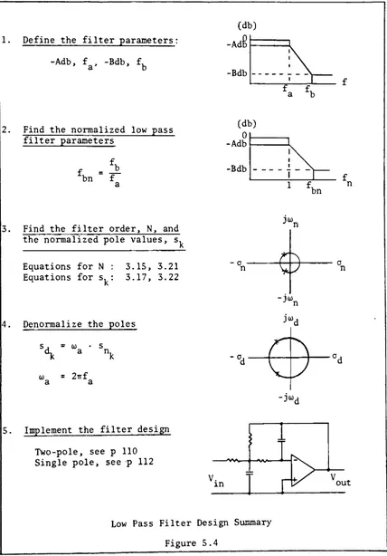
108

5.2

Low

Pass

IGMF

Active

Filter

(two-pole)

110

5.3

Low

Pass

Active

Filter

(single pole)

112

5.4

Low Pass

Filter

Design

Summary

113

Figure

Description

Page

5.6

Normalized

Low

Pass

Filter

(derived from

figure

5.5)

115

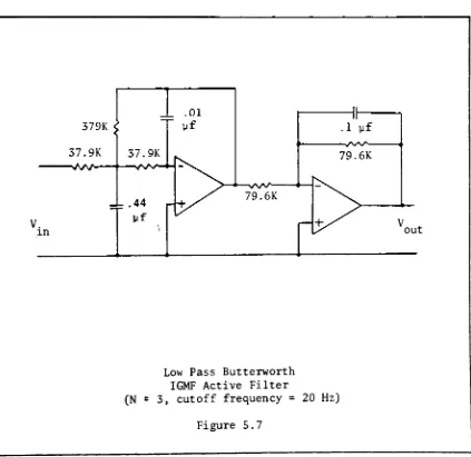
5.7

Low

Pass

Butterworth

IGMF Active

Filter

(N

3,

cutoff

frequency

20

Hz)

118

5.8

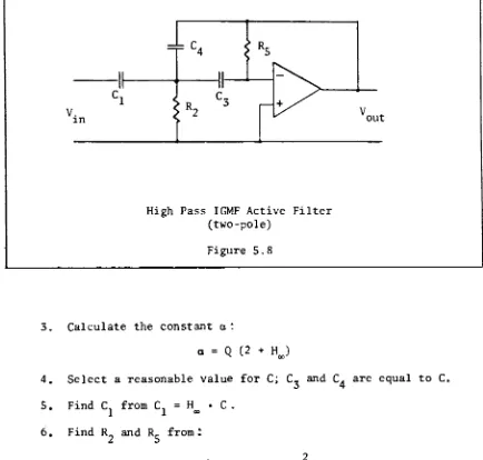
High Pass

IGMF Active Filter

(two-pole)

[

120

5.9

High Pass

Active

Filter

(single pole)

121

5.10

High Pass

Filter

Design

Summary

123

5.11

Band Pass

IGMF Active Filter

(two-pole)

125

5.12

Band

Pass

Filter

Design

Summary

126

5.13

Band Pass

Filter Requirements

(example)

127

5.14

Normalized

Low

Pass

Filter

128

5.15

Butterworth Band Pass

IGMF

Active

Filter

(f

455

KHz,

B

10

KHz,

N

2)

132

5.16

Band

Stop

IGMF

Active

Filter

(two-pole)

134

5.17

Butterworth

Band

Stop

Filter

Requirements

(example)

138

5.18

Normalized

Low

Pass

Filter

(derived

from figure

5.17)

139

5.19

Butterworth

IGMF

Band

Stop

Filter

(two-pole

example)

143

5.20

Band

Stop

Filter Design

Summary

144

CHAPTER

VI

THE

FILTER PROGRAM

6.1

Program Filter

Architecture

150

CHAPTER

VII

(refer

to

the

List

of

Illustrations

in

the

User's

Manual)

159

APPENDIX A

DEVELOPMENT

OF

THE

SOLUTIONS

FOR

THE

ELLIPTIC

FUNCTION

POLES AND

ZEROS

A.l

Denormalized

Elliptic

Filter

Response

197

Figure

Description

Page

A.

3

Prescribed Characteristics

of

the

Normalized

Elliptic

Function,

K,M

202

A.

4

Characteristics

of

the

Normalized Elliptic

Rational

Function

205

A.

5

Integrand Function

of

the

Elliptic

Integral

210

A.

6

Elliptic

Integral

Values

(Real)

as

a

Function

of

the

Amplitude,

0

211

A.

7

The

Pass

Band

of

the

Elliptic

Filter Transformed

by

the

Elliptic

Integral

(N

odd

5)

213

A. 8

The Pass

Band

of

the

Elliptic

Filter

Transformed

by

the

Elliptic

Integral

(N

even

6)

215

APPENDIX

B

PROCEDURE

FOR DETERMINING THE

NORMALIZED

ELLIPTIC

POLES

AND

ZEROS

B.l

Normalized

Low

Pass

Filter

Parameters

(parameter

basis

for

an

elliptic

filter

design)

222

B.2

Elliptic

Low

Pass

Filter

Requirements

232

B.3

Normalized

Low

Pass

Elliptic

Filter

(example)

233

B.4a

Normalized

Low

Pass

Elliptic

Filter

(N

6)

241

B.4b

Normalized

Poles/Zeros

for

the

Low

Pass

Elliptic

Filter

(N

6)

241

B.5

Normalization

with

respect

to

the

Center

Frequency

vs.

LIST OF

TABLES

Table

No.

Description

Page

2.1

Parameter

Definitions

of

the

Magnitude

Response

(Low Pass

and

High

Pass)

29

2.2

Parameter

Definitions

of

the

Magnitude

Response

(Band Pass

and

Band

Stop)

34

B.l

Elliptic

Design

Summary

Work Sheet

229

B.2

Elliptic Design

Summary

Work

Sheet

(Example)

238

D.l

Elliptic

Integral

Tables

254

CHAPTER

I

INTRODUCTION

1.1

Historical

Introduction

and

Comments

The

science

of

signal

filtering

has

evolved

from its

infancy

66

years

ago

to

a

present

day

design

technology.

Inherent

in

this

growth

has been

the

determination

of

network

theorists

to

develop

new

filter

concepts

and

design

procedures.

A

multitude

of

information

sources

and

computer

programs

have

evolved

to

such

purpose.

For

some

engineers

this

represents

a

variety

of

solutions

while

to

others

an

informational

di

lemma.

Even

with

all

this,

there

are

still

areas

in

filter design

which

remain

undeveloped.

Let

us

briefly

examine

the

historical

background

of

network

and

filter design

synthesis

and

then

examine

the

needs

which

exist

in

this

field

today.

The

concept

of

an

electric

filter

was

initially

proposed

in

1915

by

K.

Wagner

of

Germany

and

G.

Campbell

of

the

United

States.

The

concepts

were

a

result

of

their

initial

work,

performed

independently,

which

re

lated

to

loaded

transmission

lines

and

classical

theories

of

vibrating

systems.

The

first

practical

method

of

filter design became

available

when,

in

1923,

0.

Zobel

proposed

a

synthesis

method

using

multiple

reactances

[l].

This

method

was

used

until

the

1950's

when

W.

Cauer

and

S.

Darlington

published

new

network

synthesis

concepts

related

to

the

use

of

rational

functions

(in

particular

the

Chebyshev

rational

func

tion)

[2].

Later,

their

concepts

were

recognized

as

the

foundation

for

modern

day

filter

design.

In

the

1960's,

network

synthesis

concepts

written

by

M.

Van

Valkenberg

[3],

L.

Weinberg

[4],

A.

Zverev

[5]

and

many

others.

These

network

synthesis

concepts,

which

resulted

in

filter

design

techniques,

became

practical

with

the

advent

of

the

digital

computer.

Prior

to

this,

complex

mathematics

related

to

solving

the

insertion

loss

characteristics

of

some

filters

were

tedious

and

not

exact.

Such

was

the

case

for

solutions

to

the

Chebyshev

rational

function

as

described

by

Darlington

and

Cauer

[2].

With the

computer,

these

solutions

were

no

longer

a

barrier

to

filter design.

As

a

result,

tables

and

graphs

became

available

to

the

engineer

for

implementing

these

complex

filter designs

[6],

[7],

Many

filter forms

and

classes

have

since

evolved

from

these

original

ideas.

Examples

of

these

filters

are

the

Butterworth, Bessel,

Chebyshev,

image

parameter,

helical,

crystal,

etc.

Today,

the

electric

filter

manifests

itself

not

only in

electrical

and

electronic

fields but

in

most

of

the

scientific

community.

For

the

layman,

the

devices

that

have

resulted

from

the

remarkable

developments

in

network

synthesis

are

literally

packed

into many

consumer

products

as

special

features

(consider

the

controls

on

stereo

players

and

recorders

as

an

example).

Yet

the

development

of

filter

concepts

and

their

appli

cations

do

not

end

here.

New

technologies

are

rapidly

developing

which

combine

the

computa

tional

power

of

the

16

bit

and

forthcoming

32

bit

microprocessors

with

filter

synthesis

concepts

[8].

Image processing

and

voice

analysis/

synthesis

are

some

examples.

These

applications

become

increasingly

practical

with

advances

in integrated

circuits

which

implement

complex

filter chip

produced

by

Datel

Intersil).

Indeed,

filter design

principles

have

set

today's

standard

in

technology.

Their

concepts

and

devices

are

used

as

research

tools

by

many fields

in

the

scientific

community.

The

concepts

of

network

synthesis

are

therefore

essential

as

a

basic

tool

for

the

engineer.

There

remains

however

a

realistic

problem

between

filter

concepts

and

filter

design.

Not

all

engineers

are

conversant

with

the

different

types,

termi

nology

and

techniques

of

filter

design.

Certainly,

the

basic

ideas

used,

such

as

those

derived from

the

theory

of

linear

systems

(Fourier,

Laplace

transforms,

etc.),

have been

presented

to

engineers.

However

the

everyday involvement

of

engineering

responsibilities

does

not

always

afford

the

opportunity

to

develop

and

make

direct

use

of

network

syn

thesis

and

filter design

concepts.

This

suggests

that

something

addi

tional,

perhaps

a

computer

program,

is

needed

to

assist

these

engineers.

Although

design

aids

such

as

tables

and

graphs

are

available

in

a

variety

of

texts,

the

design methodology

often

remains

buried in

complex

analy

ses.

Those

who

are

involved

"with

filter design

realize

that

such

types

as

the

elliptic

function

filters

are

not

practical

without

a

computer

due

to

the

complexity

and

precision

of

the

mathematics

involved.

In

light

of

these

problems,

computer

programs

have been

written

to

aid

the

filter de

sign

process

[9],

[10].

Many

of

these

programs

are

useful

but very

limited.

Most

consider

only

a

particular

form

or

type

of

filter

such

as

the

low

pass

Butterworth

or

Chebyshev

approximations.

There

are

other

filter

types

remaining

such

as

the

high

pass,

band

pass

and

band

stop

(reject).

Still,

other

approximations

exist

for

each

of

the

above

fil

person

then

realizes

that

there

remains

a

need

for

a

computer

program

which

combines

the

filter

types

and

approximations

used

often

by

engi

neers.

This

program

should

assimilate

all

the

facts,

parameter

variabili

ty,

precision

and

design

techniques

into

one

source

which

could

be

drawn

upon

as

a

practical

tool.

The

days

of

research

involved

in evaluating

various

filter

types

and

their

performance

would

then

be

minimized.

Such

is

the

purpose

of

this

thesis.

1.2

Thesis

Objective

and

Scope

The

objective

of

this

thesis

is

to

develop

a

computer

program

which

could

be

used

by

engineers

as

a

practical

design

tool

for

electronic

active

filter

analysis

and

design

in

the

frequency

domain.

The

result

of

this

effort

is

a

computer

program

called

FILTER

which

assimilates

into

one

comprehensive

algorithm

the

filter designs

used

often

by

engineers.

The

program

FILTER implements

the

low

pass,

high

pass,

band

pass

and

band

stop

magnitude

responses

using any

of

three

classical

approximations:

Butterworth,

Chebyshev

and

elliptic

(Cauer).

The

complex

mathematics,

sorting

of

parameters

and

numerous

iterations

involved

in

these

designs

are

transparent

to

the

user

of

the

program.

Instead,

the

user

experiences

a

simple

interactive

session

which

guides

the

design

process

from

the

initial

step

of

defining

the

parameters

of

the

magnitude

response

to

the

final

step

of

component

selection

for

an

active

filter

circuit

configura

tion.

To

supplement

this

design

program,

this

thesis

text

is

provided.

The

scope

of

the

text

is

limited

to

the

design

concepts

of

filters

in

the

frequency

domain.

The

thesis

text

begins

with

the

basic definitions

and

approxi-mations

and

culminates

with

a

design methodology

for

the

basic

filter

types.

These design

concepts

are

well

established

with

the

exception

of

the

elliptic

function

design

procedure.

One

of

the

major

efforts

in

this

thesis

was

the

development

of

an

elliptic

function

design

method.

After analyzing

the

various

sources

of

literature,

it

was

evident

that

the

elliptic

design

procedures

were

quite

complex,

incomplete

and

disseminated.

Much

remained

between

the

theory

and

a

practical

design

procedure.

Because

the

mathematics

are

complex,

involving

elliptic

integrals

and

elliptic

trigonometric

functions,

a

computer

program

would

be

a

necessity

for

implementing

the

elliptic

fil

ter

on

a

practical

basis.

Programs have

been

written

for

elliptic

func

tion

filters but

again

they

are

limited in

scope,

remain

undocumented

in

analysis

and

method

or

are

just

unavailable

due

to

some

propriety.

A

clearly

stated

elliptic

design procedure,

even

if complex, is presently

needed.

This

is especially

true

for

active

filter

design.

R.

W.

Daniels

has

presented

active

filter

concepts

in his

text[l0].

His

text

is

a

most

informative

source

on

elliptic

design

since

it includes both

programs

and

analyses

pertaining

to

elliptic

parameters.

Yet

a

definitive

procedure

with

analytical

support

still

remains

somewhat

nebulous

for his

solutions

to

the

elliptic

integral

and

elliptic

sine.

These

uncertainities

have

been

clarified

and

developed

within

this

text.

An

elliptic

design

method

is

presented

in

this

thesis

and

is imple

mented

by

the

FILTER

program.

The

methods

are

based

upon

the

elliptic

function

theory

presented

by

A.

J.

Grossman

in his

article

"Synthesis

of

Tchebycheff Parameter

Symmetrical

[ll]

.

Interestingly^

his

through

with

the

determination

of

the

poles

and

zeros.

This

is

one

of

the

most

important

steps

in

filter

design.

His discussion however

was

limited

to

odd

order

functions

and

did

not

derive

solutions

to

the

elliptic

sine

or

integral.

His

interpretation,

nonetheless,

was

clearly

presented.

In

this

thesis,

the

concepts

presented

by

Grossman

are

ex

panded

to

include

the

total

design

process

of

any

order

low

pass

through

band

stop filters.

The

active

filter implementation

technique

used

is

based

upon

the

concepts

presented

by

R.

W.

Daniels[lO].

His

concepts

were

expanded

here

to

include

multiple

iterations

of

reasonable

component

values

as

a

solution

to

implementing

a

larger

range

and

optimization

of

elliptic

filters.

In

summary,

it

is

hoped

that

the

program

FILTER

along

with

this

text,

offer

a

practical

design

tool

and

reference

for

those

filter

types

most

often

used

by

engineers

in

small

signal

processing.

In

addition,

the

development

of

the

elliptic

function design

procedure

will

hopefully

promote

its

use.

The

following

is

a

discussion

on

the

organization

and

purpose

of

the

chapters

within

the

thesis

text.

1.3

Thesis

Organization

This

text

starts

with

the

fundamental

concepts

of

filters

and

builds

into

a

final

design

methodology.

With this

in mind,

the

contents

of

the

remaining

text,

6

chapters

in all,

will

now

be

discussed.

Chapter

II

provides

an

overview

of

the

basic

filter

concepts

which

are

commonly drawn

upon

throughout

the

text.

The

terminology

and

graphi

cal

representations

of

the

four filter

types

are

presented.

These

types

types

are

discussed from

an

ideal

point

of

view.

Subsequently

the

realistic

forms

and

their

terminology

are

presented.

This

leads

to

the

transfer

function,

H(s)

which

conveniently

describes

the

total

filter

response

(magnitude

and

phase)

Chapter

III

introduces

the

concept

of

the

normalized

low

pass

fil

ter.

The

importance

of

the

normalized

low

pass

filter

as

the

focal

point

of

the

design

process

is

established.

In

this

normalization

process,

methods

are

shown

for converting

each

of

the

four filter

types

into

the

normalized

low

pass

form.

The

concept

of

the

insertion

loss

function is

also

presented.

These

concepts

are

then

expanded

to

con

sider

the

Butterworth,

Chebyshev

and

elliptic

function

approximations

in

their

normalized

low

pass

form.

Their

magnitude

and

phase

responses

are

considered

along

with

the

pole/zero

locations

on

the

s-plane.

Compari

sons

are

then

made

among

these

filter

characteristics.

As

a

result

of

these

discussions,

the

reader

should

develop

an

intuitive

feeling

for

the

differences in

the

magnitude

responses

and

their

advantages

or

dis

advantages.

In

the

design process,

where

the

normalized

low

pass

filter

is

used,

a

person

then

realizes

the

choice

among

the

three

approximations

to

meet

his/her design

specifications.

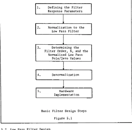
Chapter

IV

describes how

the

normalized

low

pass

filter

relates

to

the

other

basic

magnitude

types

such

as

high pass,

band

pass

and

band

stop filters.

These

relationships,

described

by

two

processes,

normali

zation

and

transformation,

are

concisely

and

mathematically

presented.

Having

determined

the

poles

and

zeros,

the

process

of

denormalization

is

presented

as

the

step

required

to

return

from

this

normalized

low

pass

needed

to

begin

the

hardware

implementation.

The

theoretical

development

of

the

design

process

is

completed

in

this

chapter.

The

steps

of

nor

malization,

transformation,

deriving

the

poles/zeros

and

denormalization

have

all

been developed

and

presented

in

chapters

II-IV.

What

is

needed

at

this

point

is

a

section

which

pulls

together

all

these

concepts

into

practical

design

methods.

Chapter V

is

a

section

on

active

filter design

methodology.

Here

the

concepts

of

normalization

through

denormalization

are

applied

for

each

filter

type

(low

pass

through

band stop)

These

methods

present

the

total

design

process

which

starts

by

defining

the

desired

filter

response

parameters

and

culminates

with

an

active

filter

circuit.

Chapter VI

introduces

the

program

FILTER.

This

program

is

a

com

prehensive

algorithm

which

implements

all

the

concepts

previously de

veloped.

This

chapter

then

describes how

the

program

is

structured

to

handle

the

design

variabilities

and

filter

responses.

A

program

map

and

general

flowchart

aid

this

discussion.

Chapter VII

is

the

user

manual

for

the

program

FILTER.

The

specifi

cations,

definitions

of

parameters

and

examples

are

given.

The

reader

should

at

least

glance

at

this

section

and

see

the

example

program

exe

cutions.

In

the

appendix,

the

development

of

the

elliptic

function design

method

is

presented

with

an

example

and

theory

of

elliptic

parameters.

This

appendix

is informative if

a

person

desires

an

in-depth

interpreta

tion

of

the

elliptic

parameters

and

how

they

relate

to

the

design

pro

CHAPTER

II

BASIC FILTER CONCEPTS

2.1

Introduction

This

chapter

provides

an

overview

of

the

fundamental

concepts

which

are

used

to

describe

the

characteristic

responses

of

the

basic

filter

types.

The

basic

filter

types

are

the

low pass, high

pass,

band

pass

and

band

stop.

This

overview

begins

with

a

discussion

of

the

magnitude

and

phase

characteristics

of

the

ideal

frequency

domain

filter.

By

using

the

ideal

form,

the

terms, definitions

and

analyses

of

the

response

characteristics

can

be

presented

without

great

complexity.

Following

this,

a

discussion

is

presented

which

explains

how

the

magnitude

shape

of

the

ideal

frequency

domain

filter is

altered

due

to

practical

limita

tions.

This

leads

to

the

straight

line

transition

diagram

which

repre

sents

the

non-ideal

or

realistic

magnitude

response

of

the

filter.

These

diagrams

are

presented

for

each

of

the

four basic

filter

types

along

with

the

symbols

and

definitions

which

are

to

be

used

commonly

throughout

the

text.

The

transfer

function, H(s)

is

then

introduced

as

a

convenient

mathematical

representation

of

the

realistic

response

of

the

filter.

The

transfer

function describes

the

magnitude

response

as

represented

with

the

straight

line

transition

diagram,

as

well

as

the

phase

response.

The

general

form

of

H(s)

is

presented.

Then

the

par

ticular

forms

of

the

transfer

functions

and

their

representations

on

the

s-plane

are

presented

for

each

of

the

four filter

types.

By

the

end

of

this

chapter,

the

reader

should

have

an

understanding

of

the

parameter

definitions

which

describe

the

magnitude

response

of

the

representations

of

the

filter

types

using

the

transfer

function,

H(s).

2.2

The

Ideal

Frequency

Domain

Filter

In

this

section

the

four basic

filter

types

(low pass, high

pass,

band

pass

and

band stop)

are

introduced in

their

ideal

form.

The

pur

pose

here

is

to

review

the

magnitude

shapes

in

the

frequency

domain

and

introduce

the

terminology

associated

with

these

filters.

Emphasis

is

placed

on

examining

the

theory

related

to

the

low

pass

filter

character

istics.

The

remaining

filter

types

are

simply

presented

without

theo

retical

involvement.

This

is because

their

ideal

nature

is

similar

to

the

low

pass

and

the

same

analytical

thought

process

applies.

2.2.1

The

Ideal

Low

Pass

Filter

Figure

2.1

illustrates

the

magnitude

and

phase

characteristics

of

the

ideal

low

pass

filter.

The

characteristics

of

the

filter

are

repre

sented

by

H(ju>)

The

input

and

output

sig

nals

are

x(t)

and

y(t)

respectively.

The

ideal

low

pass

filter

and

any ideal

filter

has

a

constant

magni

tude

in

the

frequency

band

of

interest

(pass

band)

This

is

rep

resented

by

|H(ju))|=A

in

the

pass

band

as

x(t)

H(ju>)

y(t)

|H(jo))|

V

A

pass

band

stop band

|H(juO|=0

-U)

0/0)

^-n

a

/a

\

0(jo))=-u)to

Ideal

Frequency

Domain

Filter

(low pass)

shown

in

figure

2.1.

Outside

of

the

pass

band

the

magnitude

is

zero.

This

region

is defined

as

the

stop band

with

|H(jo>)|=0

as

shown

in

figure

2.1.

The

ideal

filter

also

responds

with

a

linear

phase

shift,

0(jo)),

throughout

the

pass

band.

Beyond

the

pass

band

the

phase

shift

is

of

no

concern

since,

ideally,

there

is

no

output

signal.

Therefore,

any

phase

shift

can

exist.

These

ideal

characteristics

can

be

summarized

for

the

low

pass

filter

as

follows:

Magnitude

|H(jo))|

A

for

<oxo)

=

₀

for

(ul

>o)

Phase

0(joi)

-o)tn

for

<oxo>

J

0

a

a

=

any

for

|oi|

>o)

3.

where

o)

refers

to

the

cutoff

frequency.

Let

us

examine

the

reason

why

the

phase

shift,

0(joi),

is

and

then

derive

the

function,

H(joj),

by

using

the

Fourier

transform.

If

it

is

assumed

that

the

filter

removes

energy from

the

input

signal,

x(t),

by

using

some

combination

of

reactive

elements,

then

the

output

signal,

y(t)

will

have

a

phase

shift

which

results

in

a

time

delay

relative

to

the

input.

Let

this

time

delay

be

designated

by

t_

seconds.

This

delay,

t-,

is

illustrated

in

figure 2.2c

where

an

input

signal

x(t)

has

been

put

through

an

ideal

low

pass

filter

to

produce

y(t)

The

input

signal,

x(t)

is

composed

of

two

separate

signals

x.

(t)

and

x2(t)

as

shown

in figure

2.2a.

x.

(t)

consists

of

frequencies

within

the

pass

band

of

the

ideal

low

pass

filter.

This

is

represented

by

X1

(o>)

in figure

2.2b.

The

signal

x2(t)

consists

of

frequencies in

Input

Ideal

Filter

Output

x(t)

H(jo>)

)

t

A

X^o))

ft

X2(o))

/

/ \

y(t)

A

t

₀

(a)

(b)

Ax1(t-tQ)

(c)

Time

Delay

(t

)

Characteristics

of

the

Ideal

Low

Pass

Filter

Figure

2.2

pass

band

signal

component,

x

(t)

altered

in

magnitude

to

A

and

time

de

layed

by

t

seconds

(figure

2.2c).

The

magnitude,

A,

is usually less

than

the

input

magnitude

unless

the

filter device

is

active.

The

fre

quency

components

in

the

stop

band, X_(oj)

as

shown

in

figure

2.2b,

have

been

totally

removed

by

the

filter.

The

time

delay,

t,

can

be

related

to

the

period,

T,

of

any

frequency

component

in

x.(t)

as

follows:

-t,

Delay

(cycles)

or

in

terms

of

phase,

0

-T

tQ

(radians)

o)

2tt/T.

Therefore,

0(jo))

-o)tQ

(2.1)

where

o)

is

any

pass

band

frequency

and

t

is

the

time

delay.

Equation

(2.1)

can

also

be

rearranged

to

determine

the.

time

delay,

t,

in

terms

of

phase

shift,

0(jo)),

as

shown

below.

_

0(ju>)T

0(jo))

1_

^0

2tt

2tt

f

Or

in

terms

of

degrees,

we

have

Time

delay

tQ

^j")

1.

(seconds)

(2.2)

where

0(jo))

is

the

phase

shift

associated

with

any

pass

band

frequency,

f.

The

group

delay,

T

is

the

slope

of

the

phase

shift,

0(ju),

at

a

particular

frequency,

o)

This

is mathematically

represented

as

Group delay

T

^IM

g

do)

0)=O)

(2.3)

x

Since

the

ideal

filter illustrated in

figure

2.1

has

the

same

phase

slope

throughout

the

pass

band,

the

group

delay

is

the

same

for

all

frequencies

and

is

found

as

follows:

for

0(joi)

0

the

group

delay

is

=

d0(jo>)

lg

where

tQ

is

the

delay

time

previously

specified

and

shown

in figure

2.2c.

Having

specified

the

pass

band

magnitude

as

A

and

the

time

delay

as

tn

seconds,

the

output

signal

y(t)

can

be

related

to

the

input

x(t)

by

y(t)

A.XjCt-tjj)

+

0.x2(t-tQ)

which

simplifies

to

Output

signal

y(t)

A-x(t-tQ)

(2.4)

The

input

and

output

signals

can

be

represented

in

the

frequency

domain

by

use

of

the

Fourier

transform.

This

will

lead

to

the

transfer

function,

H(joj)

for

the

ideal

low

pass

filter.

For

the

input

signal

x1 (t)

existing

for

time

T,

the

Fourier

transform

is

F[x(t)]

X(o>)

J

x(t)

e"jutdt

Since

x(t)

xx(t)

+

x2(t)

and

by

use

of

the

superposition

principle,

we

have

F[Xl(t)

+

x2(t)]

=/

Xl(t)

e^dt

J

x2(t)

e"ja,tdt

(2.5)

For

the

output

signal,

y(t)

,

the

transform is

{T+t0

y(t)

e"jutdt

'0

Substituting

y(t)

Ax^t-t^

from

equation

(2.4)

into

Y(o))

we

have

,T+t0

Y(o))

AXjCt-tjj)

e-ja)tdt

(2.6)

*0

Letting

T

t-tQ,

then

t

T+tQ

and

dt

dT

If

the

expressions

T

t-tQ

and

dt

dT

are

substituted

into

equation

(2.6)

for

Y(oi)

then

P

=

1

Ax2

Jo

-jo)(T+t

)

Y(o))

I

Ax.

(T)

e

U

dT

>T

jo)tQ

|

Y(o))

A-e

I

x1(T)

e

dT

(2.7)

H(jo))

X^oi)

The

right

hand

portion

of

equation

(2.7)

was

previously

shown

to

be

Xj(o))

in

equation

(2.5).

Thus

the

Fourier

transform

of

the

output

signal

is

-jut

Y(o))

Ae

u

Xx(o))

(2.8)

-jut

where

the

time

delay

is

represented

in

the

frequency

domain

as

e

The

transfer

function

of

the

ideal

low

pass

filter is

then

found

from

=

1M

iHf,.,..,i

H(j)

Y^f

lH^^l

which

yields

J

C-*t

)

H(jo>)

Ae

u

(2.9)

The

representation

of

the

ideal

low

pass

filter

with

its

transfer

func

tion

is depicted in

the

following

section

in

figure

2.3.

2.2.2

Summary

of

the

Ideal

Low

Pass Filter Characteristics

Let

us

summarize

the

characteristics

which

have

been

determined

for

the

ideal

low

pass

filter.

Figure

2.3

illustrates

these

character

istics.

This

figure is

similar

to

figure 2.1

and

is

presented

here

in

x(t)

X(o))

-joit.

Ae

H(jo))

|H(jo.)|e

j0(jo>)

=

Ae

y(t)

Y(o))

0

The

Transfer Function

(a)

-O)

H(jo))

d0(joQ

do)

0

0(jo>)

0

Magnitude

and

Phase

Characteristics

(b)

+0)

Summary

of

the

Ideal

Low

Pass

Filter

Characteristics

The

magnitude

characteristics,

as

shown

in

figure

2.3b,

were

de

scribed

as

|H(jo))|

A

for

<oxo)

3-

3.

=