Planning in answer set programming while learning action costs for mobile robots

This is a repository copy of

Planning in answer set programming while learning action

costs for mobile robots

.

White Rose Research Online URL for this paper:

http://eprints.whiterose.ac.uk/101400/

Version: Accepted Version

Proceedings Paper:

Yang, F, Khandelwal, P, Leonetti, M orcid.org/0000-0002-3831-2400 et al. (1 more author)

(2014) Planning in answer set programming while learning action costs for mobile robots.

In: Knowledge Representation and Reasoning in Robotics. AAAI 2014 Spring Symposia,

24-26 Mar 2014, Palo Alto, California USA. AAAI , pp. 71-78. ISBN 9781577356455

© 2014, Association for the Advancement of Artificial Intelligence. This is an author

produced version of a paper published in Knowledge Representation and Reasoning in

Robotics.

[email protected] https://eprints.whiterose.ac.uk/ Reuse

Unless indicated otherwise, fulltext items are protected by copyright with all rights reserved. The copyright exception in section 29 of the Copyright, Designs and Patents Act 1988 allows the making of a single copy solely for the purpose of non-commercial research or private study within the limits of fair dealing. The publisher or other rights-holder may allow further reproduction and re-use of this version - refer to the White Rose Research Online record for this item. Where records identify the publisher as the copyright holder, users can verify any specific terms of use on the publisher’s website.

Takedown

If you consider content in White Rose Research Online to be in breach of UK law, please notify us by

Planning in Answer Set Programming while Learning Action Costs

for Mobile Robots

Fangkai Yang, Piyush Khandelwal, Matteo Leonetti and Peter Stone

Department of Computer Science The University of Texas at Austin

2317 Speedway, Stop D9500 Austin, TX 78712, USA

{fkyang,piyushk,matteo,pstone}@cs.utexas.edu

Abstract

For mobile robots to perform complex missions, it may be necessary for them to plan with incomplete informa-tion and reason about the indirect effects of their ac-tions. Answer Set Programming (ASP) provides an el-egant way of formalizing domains which involve indi-rect effects of an action and recursively defined fluents. In this paper, we present an approach that uses ASP for robotic task planning, and demonstrate how ASP can be used to generate plans that acquire missing information necessary to achieve the goal. Action costs are also in-corporated with planning to produce optimal plans, and we show how these costs can be estimated from expe-rience making planning adaptive. We evaluate our ap-proach using a realistic simulation of an indoor envi-ronment where a robot learns to complete its objective in the shortest time.

Introduction

Automated planning provides great flexibility over direct implementation of behaviors for robotic tasks. In mobile robotics, uncertainty about the environment stems from many sources. This is particularly true for domains inhab-ited by humans, where the state of the environment can change outside the robot’s control in ways hard to pre-dict. Probabilistic planners attempt to capture this complex-ity, but planning in probabilistic representations makes rea-soning much more computationally expensive. Furthermore, correctly modeling the system using probabilities is more difficult than representing knowledge symbolically. Indeed, robotic planning systems are frequently based on symbolic deterministic models, and execution monitoring. The brittle-ness owing to errors in the model and unexpected conditions are overcome through monitoring and replanning.

Automated symbolic planning includes early work such as situational calculus (McCarthy and Hayes 1969), STRIPS (Fikes and Nilsson 1971), ADL (Pednault 1989); recent ac-tion languages such as C+ (Giunchiglia et al. 2004) and BC (Lee, Lifschitz, and Yang 2013); and declarative pro-gramming languages such as Prolog and logic propro-gramming based on answer set semantics (Gelfond and Lifschitz 1988;

Copyright c2016, Association for the Advancement of Artificial Intelligence (www.aaai.org). All rights reserved.

1991). The latter is also referred to as Answer Set Program-ming (ASP). These languages allow users to formalize dy-namic domains as transition systems, by a set of axioms that specify the precondition and effects of actions and the rela-tionship between state variables. In ASP, the frame problem (McCarthy and Hayes 1969) can be solved by formalizing the commonsense law of inertia.

Compared to STRIPS or PDDL-style planning languages, ASP and action languages provide an elegant way of formal-izing indirect effects of actions asstatic laws, and thus solve the ramification problem (Lin 1995). Although the original specification of PDDL includes axioms (which correspond to non-recursive static laws in our terminology), the seman-tics for these axioms are not clearly specified. Indeed, in most planning domains investigated by the planning com-munity and in planning competitions, no axioms are needed.

Thi´ebaux et al.(Thi´ebaux, Hoffmann, and Nebel 2003) ar-gued that the use of axioms not only increases the expres-siveness and elegance of the problem representation, but also improves the performance of the planner. Indeed, in recent years, robotic task planning based on ASP or related ac-tion languages has received increasing attenac-tion (Caldiran et al. 2009; Erdem and Patoglu 2012; Chen et al. 2010; Chen, Jin, and Yang 2012; Erdem et al. 2013; Havur et al. 2013).

We evaluate our approach using a simulated mobile robot navigating through an indoor environment and interacting with people. Should certain information necessary for com-pleting a task be missing, the planner can issue a sensing action to acquire this information through human-robot in-teraction. By integrating the planner with a learning module, the costs of actions are learned from plans’ execution. Since the only interface between the planner and the learning mod-ule is through costs, the action theory is left unchanged, and the proposed approach can in principle be applied to any metric planner. All the code used in this paper has been im-plemented using theROS middleware package (Quigley et

al. 2009), and the realistic 3D simulator GAZEBO(Koenig and Howard 2004), and is available in the public domain1_.

Related Work

In recent years, action languages and answer set pro-gramming have begun to be used for robot task planning (Caldiran et al. 2009; Erdem and Patoglu 2012; Erdem et al. 2013; Havur et al. 2013). In these previous works, domains are small and idealistic. The planning paradigm is typical classical planning with complete information, and shortest plans are generated. Since the domains are small, it is possi-ble to use grid worlds so that motion control is also achieved by planning. In contrast, we are interested in large and con-tinuous domains, where navigation is handled by a dedicated module to achieve continuous motion control, and require planning with incomplete information by performing knowl-edge acquisition through human-robot interaction.

The work of Erdem et al. (Erdem, Aker, and Patoglu 2012) improves on existing ASP approaches for robot task planning by both using larger domains in simulation, as well as incorporating a constraint on the total time required to complete the goal. As such, their work attempts to find the shortest plan that satisfies the goal within this time con-straint. In contrast, our work attempts to explicitly minimize the overall cost to execute the plan (i.e. the optimal plan), instead of finding the shortest plan. Another difference be-tween the two approaches is that Erdem et al. attempt to include geometric reasoning at the planning level, i.e. the ASP solver considers a coarsely discretized version of the true physical location of the robot. Since we target larger domains, we discretize the location of the robot at the room level to keep planning scalable and use dedicated low-level control modules to navigate the robot.

The difficulty in modeling the environment has motivated a number of different combinations of planning and learning methods. The approach most closely related to ours is the PELA architecture (Jimnez, Fernndez, and Borrajo 2013). In PELA, a PDDL description of the domain is augmented with cost information learned in a relational decision tree (Blockeel and De Raedt 1998). The cost computed for each action is such that the planner minimizes the probability of plan failures in their system. We estimate costs based on any metric observable by the robot. Some preliminary work has been done in PELA to learn expected action durations (Quintero et al. 2011), using a variant of relational decision

1

https://github.com/utexas-bwi/bwi_planning

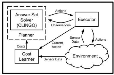
Figure 1: The architecture implemented in our approach. The planner invokes a cost estimator that learns the actual action costs from the sensor data during execution.

trees. Differently, we learn costs simply using exponentially weighted averaging, which allows us to respond to recent changes in the environment. Furthermore, while that work is specific to PDDL-style planners, we perform the first inte-gration between ASP and learning, at the advantage of defin-ing indirect effects of actions and recursively defined fluents as planning heuristics.

Architecture Description

Our proposed architecture (shown in Figure 1) has two mod-ules that comprise the decision making: a planning module, and a cost estimation module. At planning time, the plan-ner polls the cost of each action of interest, and produces a minimum plan. The planner itself is constituted by a do-main description specified in ASP and a solver, in our case

CLINGO(Gebser et al. 2011a). After plan generation, an ex-ecutor invokes the appropriate controllers for each action, and grounds numeric sensor data into symbolic fluents, for the planning module to verify. If the observed fluents are incompatible with the state expected by the planner, replan-ning is triggered. During action execution, the cost estimator receives the sensor data, and employs a learning algorithm to estimate the value of the expected cost of each action from the experienced samples.

This architecture allows to treat the planning module as a black box, and can in principle be adopted with any met-ric planner. For the same reason, the formalism used to rep-resent the state space in the planner and the cost estimator modules need not be same. In the following sections, we give a detailed description of the different elements of the system.

Domain Representation

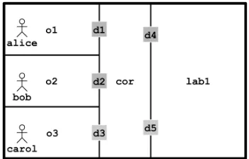
Figure 2:The layout of the example floor plan with an overlay of the rigid knowledge provided to the planner.

Formalizing the Dynamic Domain

Domain knowledge about a building includes the follow-ing four different types of information: rigid knowledge,

time-dependent external knowledge, time-dependent inter-nal knowledgeandaction knowledge. We explain each of these in detail in the following subsections. All rules formal-izing aspects of the domain are presented using syntax from

GRINGO (Gebser et al. 2011b). Due to space constraints, some portions of the ASP encoding are not present and can be viewed online in our code base.

Rigid knowledge includes information about the building that does not depend upon the passage of time. In other words, as the robot moves around inside the building, rigid knowledge should not change. In our example, rigid knowl-edge includes information about offices, labs, corridors, doors, and accessibility between all these locations. It also includes information about building residents, their occupa-tions, the offices to which they are assigned, and whether a person knows where another person is. Rigid knowledge has been formalized in our system using the following pred-icates:

• office(X),door(Y),room(Z):Xis an office,Yis a door andZis a room.

• hasdoor(X,Y): roomXhas doorY.

• acc(X,Y,Z): room X is accessible from room Z via doorY.

• indacc(X,Y,Z): roomXis indirectly accessible from roomZvia doorY.

• secretary(X),faculty(Y), person(Z): X is a secretary,Yis a faculty, andZis a person.

• in office(X,Y): personXis assigned to officeY. • knows(X,ploc(Y)): personXknows the location of

personY.

The following rules define the rigid knowledge in the exam-ple environment illustrated in Fig. 2:

room(cor).

office(o1;;o2;;o3;;lab1). room(X):- office(X). door(d1;;d2;;d3;;d4;;d5). hasdoor(o1,d1;;o2,d2;;o3,d3;;

lab1,d4;;lab1,d5).

secretary(carol). faculty(alice;;bob).

in_office(alice,o1;;bob,o2;;carol,o3). knows(carol,ploc(X)):- faculty(X). person(X) :- faculty(X).

person(X) :- secretary(X).

We also define additional rules that define accessibility in-formation between 2 rooms:

acc(X,Y,cor):- room(X),door(Y),hasdoor(X,Y). acc(Z,Y,X):- acc(X,Y,Z).

indacc(X,Y,Z):- acc(X,Y,Z).

indacc(X,Y,Z):- acc(X,Y,Z1),indacc(Z1,Y1,Z).

It is important to notice thatindaccis recursively de-fined by the last rule above, which is usually not easily achieved in a PDDL-style language. Later we will show that

indaccis used to formulateplanning heuristicswhich sig-nificantly shorten planning time.

Time-dependent external knowledge includes informa-tion about the environment that can change over time and cannot be affected by the robot’s actions. For the example environment, time-dependent external knowledge is formal-ized as follows:

• The current location of a person is formalized by the flu-entinside.inside(X,Y,I)means at time instantI, personXis located in roomY.

• By default, a person is inside the office that he is assigned to:

inside(X,Y,0):- in_office(X,Y), not -inside(X,Y,0).

In the above rule we used two kinds of negation: - is known as strong negation (classical negation) in ASP lit-erature (Gelfond and Lifschitz 1991), which is the same as the negation sign¬in classical logic, andnotis known as

negation as failure(Gelfond and Lifschitz 1988), which is similar to the negation in Prolog and intuitively under-stood asthere is no evidence.

• A person can only be inside a single room at any given time:

-inside(X,Y,I):- inside(X,Y1,I), Y1!=Y, room(Y).

• insideis aninertial fluent. An inertial fluent is a fluent whose value does not change by default. These two rules formalize the commonsense law of inertia for the fluent

inside:

inside(X,Y,I+1):- inside(X,Y,I),

not -inside(X,Y,I+1), I<n. -inside(X,Y,I+1):- -inside(X,Y,I),

not inside(X,Y,I+1), I<n.

wherendenotes maximum possible time steps. To solve a planning task, the value ofnspecifies the upper-bound on the number of steps in the plan.

• open(X,I): a doorXis open at timeI. By default, a door is not open.

-open(X,I):- not open(X,I), door(X).

• facing(X,I): the robot is next to and facing doorXat timeI. The fluent is inertial. The robot cannot face two different doors simultaneously.

facing(X,I+1):- facing(X,I),

not -facing(X,I+1), I<n. -facing(X,I+1):- -facing(X,I),

not facing(X,I+1), I<n. -facing(X2,I):- facing(X1,I), X1!=X2,

door(X2),I<=n.

• beside(X,I): the robot is next to door Xat time I.

besideis implied byfacing, but not the other way around. The fluent is inertial. The robot cannot be beside two different doors simultaneously.

beside(X,I):- facing(X,I). beside(X,I+1):- beside(X,I),

not -beside(X,I+1), I<n. -beside(X,I+1):- -beside(X,I),

not beside(X,I+1), I<n. -beside(X2,I):- beside(X1,I), X1!=X2,

door(X2),I<=n.

Since besideis implied byfacing, it is an indirect effect of any actions that affectfacing.

• at(X,I): the robot is at roomXat timeI.atis inertial, and the robot must be at exactly one location at a given time.

{at(X,I+1)}:- at(X,I), room(X), I<n. :- not 1{at(X,I):room(X)}1.

• visiting(X,I): the robot is visiting a person X at timeI. By default, a robot is not visiting anyone.

-visiting(X,I):- not visiting(X,I), person(X).

Action knowledge includes the rules that formalize robot actions, the preconditions to execute these actions, and the effects of these actions. Actions are divided intonon-sensing

andsensing actions. Non-sensing actions change the state of the world, for instance a robot can approach a door and change its own location. On the other hand, sensing actions don’t change the state of the world and are executed to ac-quire missing information. The robot has four non-sensing actions:

• approach(X,I): the robot approaches door X at timeI. A robot can only approach a door accessible from its current location if it is not facing the door already. Ap-proaching a door should result in the robot facing that door.

:- approach(Y,I), at(X,I),

{door(Y):acc(X,Y,Z)}0, I<n. :- approach(X,I), facing(X,I), I<n.

facing(X,I+1):- approach(X,I),door(X),I<n.

• gothrough(X,I): the robot goes through door X at timeI. The robot can only go through a door if the door is accessible from the robot’s current location, if it is open, and if the robot is facing it.

:- gothrough(Y,I), at(X,I),

{door(Y):acc(X,Y,Z)}0, I<n. :- gothrough(Y,I), not open(Y,I), I<n. :- gothrough(Y,I), not facing(Y,I), I<n.

Executing thegothroughaction results in the robot’s location being changed to the connecting room and the robot no longer facing the door.

at(Z,I+1):- gothrough(Y,I),

at(X,I), acc(X,Y,Z), I<n. -facing(Y,I+1):- gothrough(Y,I),

at(X,I), acc(X,Y,Z), I<n.

• greet(X,I): the robot greets person X at time I. A robot can only greet a person if both the robot and that person are in the same room. Greeting a person results in thevisitingfluent being true.

:- greet(X,I), at(Y,I), inside(X,Y1,I), Y!=Y1, I<n. visiting(X,I+1):- greet(X,I), I<n.

• opendoor(X,I): the robot opens a closed door Xat timeI. The robot can only open a door that it is facing.

:- opendoor(X,I), not facing(X,I), I<n. :- opendoor(X,I), open(X,I), I<n.

open(X,I+1):-opendoor(X,I),-open(X,I),I<n.

The robot has one sensing action:

• askploc(X,I): The robot asks the location of personX

at time I if it does not know the location of personX. Furthermore, the robot can only execute this action if it is visiting a personYwho knows the location of personX. The resulting state should include the location of personX

entered by personYas roomZ.

:- askploc(X,I), inside(X,Y,I), I<n. :- askploc(X,I),

{visiting(Y,I):person(Y)}0, I<n. :- askploc(X,I), visiting(Y,I),

not knows(Y,ploc(X)), I<n.

1{inside(X,Z,I+1):room(Z)}1:-askploc(X,I), I<n.

Also included are a set of constraints that forbid concur-rent execution of actions and a set of choice rules such that at any time, executing any action is arbitrary. We present only one example of a choice rule below which formalizes that at any timeI<n, the robot has the right to approach a doorX.

{approach(X,I)}:- door(X), I<n.

Generating and executing plans

The planner first queries the robot for its initial state, which is returned through sensing in the form of observable fluent values forat,beside,facingandopen:

at(lab1,0) -beside(d4) -beside(d5) ...

The sensors guarantee that the values for at is always returned for exactly one location, andbesideandfacing

are returned with at most one door.

With the initial state available, the planner uses the answer set solverCLINGOto plan the steps for achieving a formally described goal. For instance, if the goal is to visit Bob, then the goal is formalized as:

To find the shortest plan for this goal, we iteratively in-crement n(starting at 1) and call the answer set solver to see if a plan exists. Since we are interested in a plan of reasonable size, we assign an upper bound to n, denoted bymax size. If a plan is not generated within this upper bound, we declare that the goal cannot be achieved. Assum-ing that the robot starts inlab1and does not face a door initially, the answer set solver successfully finds the follow-ing plan whenn=7:

approach(d4,0) opendoor(d4,1) gothrough(d4,2) approach(d2,3) opendoor(d2,4) gothrough(d2,5) greet(bob,6)

These atoms represent the plan and are executed on the robot one at a time. The answer set also contains atoms that represent world transitions, such as:

at(lab1,0) -open(d4,0) -facing(d4,0) at(lab1,1) -open(d4,1) facing(d4,1) at(lab1,2) open(d4,2) facing(d4,2) ...

These atoms can be used to monitor execution. Exe-cution monitoring is important since it is possible that the action being currently executed by the robot does not complete successfully. In that case, the robot may re-turn observations different from the expected effects of the action. For instance, let’s assume that the robot is currently executing approach(d4,0). The robot at-tempts to navigate to door d4, but fails and returns an observation -facing(d4,1). Since this observation does not match the expected effect of approach(d4, t), which is facing(d4,1), the robot incorporates

-facing(d4,0)as part of a new initial state and replans.

Planning with incomplete information

Planning can also account for incomplete information, as the robot can sense missing information from the environ-ment. Consider a visiting faculty named Dan who is inside the building. The robot needs to visit Dan, but does not know where he is. However, the robot is aware that Carol knows the location of all faculty inside the building, and the gen-erated plan includes visiting her to acquire Dan’s location. The goal of such a plan is described below:

faculty(dan).

:- not visiting(dan, n).

We call CLINGO with this goal to generate the shortest plan. Assuming again that the robot is insidelab1, when

n=9,CLINGOreturns the answer set which contains the fol-lowing actions:

approach(d4,0) opendoor(d4,1) gothrough(d4,2) approach(d3,3) opendoor(d3,4) gothrough(d3,5) greet(carol,6) askploc(dan,7) greet(dan,8)

It is important to note that the robot greets Dan immedi-ately after asking Carol for his location, without moving to a different room. This plan is returned because the answer set contains the following atom:

inside(dan,d3,8)

This atom is the effect of executing sensing action

askploc(dan,7). Since we search for the shortest plan by incrementing the value of steps n, Dan being located in the same office as Carol facilitates the generation of the shortest plan. Therefore, at plan generation time, this miss-ing information isassumed optimistically.

As before, the plan is executed and the execution is mon-itored. The robot executes action askploc(dan,7) by asking Carol for Dan’s location. The robot obtains Carol’s answer as an atom, for instance, inside(dan,o1,8), which contradicts the optimistic assumption. Similar to exe-cution failures, a replan is called with a new initial state that contains:

inside(dan,o1,0)

After runningCLINGOagain, a new plan is found:

approach(d3,0) opendoor(d3,1) gothrough(d3,2) approach(d1,3) opendoor(d1,4) gothrough(d1,5) greet(dan,6)

It is important to note that in this scenario, formalizing sensing actionaskplocis essential to achieve the task of visiting Dan. Without this action, no plan can be found be-cause no other action can generate knowledge about Dan’s location. On the other hand, even ifaskplocis formalized to have multiple effects, only those that contribute to finding the shortest plans can occur in the plan, and the plan is re-vised during execution. This paradigm is different from con-ditional planning with sensing actions (Son, Tu, and Baral 2004), where all outcomes of sensing actions are generated off-line to obtain a tree-shaped plan, which is exponentially larger than a linear plan.

Planning with costs

In the previous section, the planner generates multiple plans of equal size out of which one is arbitrarily selected for ex-ecution. In practice, those plans are not equivalent because different actions in the real world have different costs. In our domain, we consider the cost of an action to be the time spent during its execution. For instance, in the example in the previous section, when the robot plans to visit Carol to acquire Dan’s location, the generated plan includes the robot exitinglab1through doord4. The planner also generated another plan of the same size where the robot could have ex-ited through doord5, but that plan was not selected. If we see the layout of the example environment in Fig. 2, we can see that it is indeed faster to reach Carol’s officeo3through doord5. In this section, we present how costs can be associ-ated with actions such that a plan with the smallest cost can be selected to achieve the goal.

Costs are functions of both the action being performed and the state at the beginning of the action. In this paper, for simplicity, we assume all actions apart fromapproachto have the following fixed costs:

cost(1,I):- sense(X,I), I<n. cost(5,I):- gothrough(X,I), I<n. cost(1,I):- greet(X,I), I<n. cost(1,I):- opendoor(X,I), I<n.

(a) Simulation inGAZEBO (b) Experiment floor plan

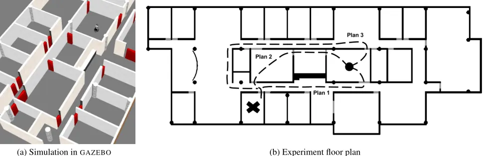
Figure 3:Final experiment domain which contains 20 rooms, 25 doors and multiple rooms with multiple doors. The circle marks the robot’s start position, the cross marks the destination. The 3 plans evaluated in the results are also marked.

cases, fluents uniquely identify the physical location of the robot in the environment as the robot moves from one door to the next. We compute the cost of approaching doorXfrom doorYin locationZas follows:

cost(@time(X,Y,Z),I):- approach(X,I),

beside(Y,I),door(X),door(Y), at(Z,I), I<n.

In our domain, the physical location of the robot is un-certain at the start of an episode. It is impossible to estimate the true cost of approaching a doorXunless the robot starts next to another door. When the robot starts next to a door, its physical location is expressed by a fluent and the true cost can be computed using the rule above. When it does not start next to a door, we assume the following fixed cost for approaching a door:

cost(10,I):- approach(X,I), {beside(Y,I)}0, I<n.

Finally, the following statement guidesCLINGOto gener-ate optimal plans in terms of the cumulative costs:

#minimize[cost(X,Y)=X@1].

As a consequence of planning with costs, the optimal plan is not necessarily the shortest one. Therefore, differ-ently from the previous section, we do not repeatedly call

CLINGOwith incremental values ofn. Rather, we call it once withndirectly assigned tomax len. Using the optimiza-tion statement above, we guideCLINGOto find the optimal answer set, i.e. the optimal plan within a size ofmax len.

Estimating costs through environment interactions

Whenever the executor successfully performs an action, the cost estimator gets asampleof the true cost for that action. It then updates the current estimate for that action using an

exponentially weighted moving average:

costk+1(X, Y) = (1−α)×costk(X, Y) +α×sample

wherekis the episode number,αis the learning rate and set to 0.5 in this paper,Xis the action, andY is the initial state. To apply this learning rule, we need estimates of all costs at episode 0. Since we want to explore a number of plans be-fore choosing the lowest-cost one, we use the technique of

optimistic initialization(Sutton and Barto 1998) and set all

initial cost estimates to a value which is much less than the true cost. This causes the robot to underestimate the cost of a plan it has not explored enough, and the robot executes it to converge the action costs to the true values. As more and more plans are explored every episode, the costs of all rel-evant actions converge to their true values, and the planner settles on the true optimal plan. Since the cost of an action is independent of the task being performed, a robot can im-prove its cost estimates while executing different goals every episode.

The exploration in optimistic initialization is short-lived (Sutton and Barto 1998). Once the cost estimator sets the values such that a particular plan becomes higher than the current best plan, the planner will never attempt to fol-low that plan even though its costs may decrease in the fu-ture. There are known techniques such as ǫ-greedy explo-ration in literature (Sutton and Barto 1998) that attempt to solve this problem. We leave testing and evaluation of these approaches to future work.

Experiments

We evaluate our approach of using ASP for plan cost min-imization and cost learning in a simulated environment whose floor plan illustrated in Figure 3b. This environment has 20 rooms, 25 doors and 5 rooms with multiple doors, and a 3D simulation for this environment was implemented us-ingGAZEBO(Koenig and Howard 2004), as depicted in Fig-ure 3a. This environment uses all the same rules presented with the example, except that it uses a much larger corpus of rigid knowledge, which can be viewed online. A simu-lated differential drive robot capable of understanding the actions described in this paper moves around inside this sim-ulation to complete goals. The robot’s interface also trans-forms any simulated sensor readings into observable fluents as required by the planner to determine if replanning is re-quired. Actions inside the simulator are not guaranteed to succeed. However, on the occasional failure, they do not fail repeatedly so that replanning can still be successful.

(a) Cost estimation during the first 30 episodes (b) Cost estimation after discovering navigation delay in episode 30 Figure 4:The cost curves of three different plans in the environment during learning.

split between 3D simulation, visualization and the planner

CLINGO.CLINGO is a monolithic system made up of two parts, the grounder GRINGO which generates variable-free programs which are then solved by the answer set solver

CLASP. In these experiments, version 3.0.3 and version 2.1.4 ofGRINGOandCLASPwere used, respectively.CLINGOwas run in parallel over 6 threads withmax lenset to 15, and was allowed 1 minute of planning time after which the best available plan was selected for execution.

In this domain, there are a large number of correct plans, and the planning time can be prohibitively long. For in-stance, there are a number of plans that go into the rooms on the top left corner of the map, or at least approach the door to that room. We remove such plans from the search space of the planner by providing the following additional heuristics along with the goal:

• Do not approach a door if that door is the only door con-necting the adjacent room to the goal of visiting Bob.

:- approach(Y,I), at(X,I), acc(X,Y,Z), 1{indacc(Z,Y1,W)}1,inside(bob,W,I), Z!=W.

Note that to formulate this constraint we use indacc, which is recursively defined in the rigid knowledge of the domain.

• Do not approach a door if the next action in the plan does not go through it. The formal definition of this heuristic has not been presented here due to its length, and can be viewed online.

These heuristics reduce the average time for finding the op-timal plan at the start of each episode from 23 to 14.275 seconds. More importantly, they greatly reduce the number of episodes required to converge learning by explicitly iden-tifying a number of plans as sub-optimal, which need not be evaluated.

We demonstrate cost learning through repeated episodes of a single-goal problem illustrated in Fig. 3b. In every episode, the robot starts at the location indicated by the cir-cle and attempts to greet a person in the location indicated

by the cross. At the end of each episode, the robot updates its estimates of action costs. Even with the heuristics mentioned above, there are still a large number of plans that can achieve this goal. For instance, there are plans that go through the seminar room and the lab as well, as without learned costs the planner has no idea that going through either of them does not shorten the distance to the goal. Although all these plans are tried out by the planner, we only present the costs for the three shortest plans after exiting each door in the ini-tial room. Plan 1 and Plan 3 are the shortest plans to achieve the goal (7 steps), and Plan 1 is also the optimal plan. Plan 2 is almost as good as the optimal plan, but requires the robot to go through 4 doors, making it longer (13 steps). In this experiment, we only learn costs for theapproachaction.

Figure 4a shows the total cost of the three plans as the cost estimates for each individual action are improved starting from the optimistically initialized values. The cost of plan 3 is significantly higher than the other two, and therefore after trying the plan once in the second episode, it is not considered again. Since the other two plans are of similar cost, their execution is interleaved until the estimate of the shortest plan converges. In some episodes, plans apart from these three are executed and the value of these plans may not change. By episode 30, the cost estimates converge such that plan 1 is always selected.

In the second experiment we show how the system can

adapt when the environment changes. Let’s assume that at episode 30, the robot starts experiencing a 20 second delay in the gray region of the map demarcated in Fig. 5, through which the optimal plan (Plan 1) passes. Consequently, the cost estimate changes and the robot switches to a different plan (Plan 2) which is now optimal, as illustrated over the next 10 episodes in the graph in Fig. 4b.

Conclusion

In this paper, we present an approach that uses ASP for robotic task planning that incorporates action costs to pro-duce optimal plans. This approach also allows to plan with incomplete information, by acquiring missing information through human-robot interaction. Furthermore, by estimat-ing costs from experience, plannestimat-ing can be adaptive to envi-ronmental changes.

Acknowledgments

The authors would like to thank Vladimir Lifschitz for many useful discussions during the seminal stages of this work. The authors would also like to thank the ROS and

GAZEBO open-source communities for infrastructure used in this work.

A portion of this research has taken place in the Learn-ing Agents Research Group (LARG) at the AI Labora-tory, University of Texas at Austin. LARG research is sup-ported in part by grants from the National Science Foun-dation (CNS-1330072, CNS-1305287), ONR (21C184-01), and Yujin Robot. LARG research is also supported in part through the Freshman Research Initiative (FRI), College of Natural Sciences, University of Texas at Austin.

References

Blockeel, H., and De Raedt, L. 1998. Top-down induction of first-order logical decision trees.Artificial intelligence (AIJ).

Caldiran, O.; Haspalamutgil, K.; Ok, A.; Palaz, C.; Erdem, E.; and Patoglu, V. 2009. Bridging the gap between high-level reason-ing and low-level control. InInternational Conference on Logic

Programming and Nonmonotonic Reasoning (LPNMR).

Chen, X.; Ji, J.; Jiang, J.; Jin, G.; Wang, F.; and Xie, J. 2010. Developing high-level cognitive functions for service robots. In

International Conference on Autonomous Agents and Multiagent Systems (AAMAS).

Chen, X.; Jin, G.; and Yang, F. 2012. ExtendingC+with composite actions for robotic task planning. InInternational Conference on Logical Programming (ICLP).

Eiter, T.; Faber, W.; Leone, N.; Pfeifer, G.; and Polleres, A. 2003. Answer set planning under action costs.Journal of Artificial Intel-ligence Research (JAIR).

Erdem, E.; Aker, E.; and Patoglu, V. 2012. Answer set program-ming for collaborative housekeeping robotics: representation, rea-soning, and execution.Intelligent Service Robotics (ISR). Erdem, E., and Patoglu, V. 2012. Applications of action lan-guages in cognitive robotics. In Erdem, E.; Lee, J.; Lierler, Y.; and Pearce, D., eds.,Correct Reasoning, volume 7265 ofLecture Notes in Computer Science. Springer.

Erdem, E.; Patoglu, V.; Saribatur, Z. G.; Sch¨uller, P.; and Uras, T. 2013. Finding optimal plans for multiple teams of robots through

a mediator: A logic-based approach.Theory and Practice of Logic Programming (TPLP).

Fikes, R., and Nilsson, N. 1971. STRIPS: A new approach to the application of theorem proving to problem solving. Artificial Intelligence (AIJ). Presented at the International Joint Conferences on Artificial Intelligence (IJCAI).

Gebser, M.; Kaminski, R.; Kaufmann, B.; Ostrowski, M.; Schaub, T.; and Schneider, M. 2011a. Potassco: The Potsdam answer set solving collection. AI Communications: The European Journal on Artificial Intelligence (AICOM).

Gebser, M.; Kaminski, R.; K¨onig, A.; and Schaub, T. 2011b. Ad-vances ingringoseries 3. InInternational Conference on Logic

Programming and Nonmonotonic Reasoning (LPNMR).

Gelfond, M., and Lifschitz, V. 1988. The stable model seman-tics for logic programming. InInternational Logic Programming Conference and Symposium (ICLP/SLP).

Gelfond, M., and Lifschitz, V. 1991. Classical negation in logic programs and disjunctive databases.New Generation Computing. Giunchiglia, E.; Lee, J.; Lifschitz, V.; McCain, N.; and Turner, H. 2004. Nonmonotonic causal theories.Artificial Intelligence (AIJ). Havur, G.; Haspalamutgil, K.; Palaz, C.; Erdem, E.; and Patoglu, V. 2013. A case study on the Tower of Hanoi challenge: Repre-sentation, reasoning and execution. InInternational Conference on Robotics and Automation (ICRA).

Jimnez, S.; Fernndez, F.; and Borrajo, D. 2013. Integrating plan-ning, execution, and learning to improve plan execution. Compu-tational Intelligence.

Koenig, N., and Howard, A. 2004. Design and use paradigms for Gazebo, an open-source multi-robot simulator. InInternational Conference on Intelligent Robots and Systems (IROS).

Lee, J.; Lifschitz, V.; and Yang, F. 2013. Action languageBC: A preliminary report. InInternational Joint Conference on Artificial Intelligence (IJCAI).

Lin, F. 1995. Embracing causality in specifying the indirect effects of actions. InInternational Joint Conference on Artificial Intelli-gence (IJCAI).

McCarthy, J., and Hayes, P. 1969. Some philosophical prob-lems from the standpoint of artificial intelligence. In Meltzer, B., and Michie, D., eds.,Machine Intelligence. Edinburgh University Press.

Pednault, E. 1989. ADL: Exploring the middle ground between STRIPS and the situation calculus. InInternational Conference on Principles of Knowledge Representation and Reasoning (KR). Quigley, M.; Conley, K.; Gerkey, B.; Faust, J.; Foote, T.; Leibs, J.; Wheeler, R.; and Ng, A. Y. 2009. ROS: an open-source robot operating system. InOpen Source Softare in Robotics Workshop at ICRA ’09.

Quintero, E.; Alc´azar, V.; Borrajo, D.; Fern´andez-Olivares, J.; Fern´andez, F.; Olaya, A. G.; Guzm´an, C.; Onaindia, E.; and Prior, D. 2011. Autonomous mobile robot control and learning with the PELEA architecture. InAutomated Action Planning for Au-tonomous Mobile Robots Workshop at AAAI ’11.

Son, T. C.; Tu, P. H.; and Baral, C. 2004. Planning with sensing actions and incomplete information using logic programming. In

International Conference on Logic Programming and Nonmono-tonic Reasoning (LPNMR).

Sutton, R. S., and Barto, A. G. 1998. Reinforcement learning: An introduction. Cambridge University Press.