Description and assessment of regional sea-level trends and variability from altimetry and tide gauges at the northern Australian coast

Elsevier Editorial System(tm) for Advances in Space Research

Manuscript Draft

Manuscript Number: ASR-D-17-00840R2

Title: Description and assessment of regional sea-level trends and variability from altimetry and tide gauges at the northern Australian coast

Article Type: ES - Earth Sciences

Keywords: Satellite radar altimetry; Mann-Kendall test; sea level trend; tide gauge, Australia.

Corresponding Author: Dr. Zahra Gharineiat, Ph.D

Corresponding Author's Institution: University of Southern Queendsland First Author: Zahra Gharineiat, Ph.D

Order of Authors: Zahra Gharineiat, Ph.D; Xiaoli Deng, Ph.D

Abstract: This paper aims at providing a descriptive view of the low-frequency sea level changes around the northern Australian coastline. Twenty years of sea level observations from multi-mission satellite altimetry and tide gauges are used to characterize sea level trends and inter-annual variability over the study region. The results show that the interannual sea level fingerprint in the northern Australian coastline is closely related to El Niño Southern Oscillation (ENSO) and Madden-Julian Oscillation (MJO) events, with the greatest influence on the Gulf

Carpentaria, Arafura Sea, and the Timor Sea. The basin average of 14 tide-gauge time series is in strong agreement with the basin average of the altimeter data, with a root mean square difference of 18 mm and correlation coefficient of 0.95. The rate of sea level rise (6.3 ± 1.4 mm/yr) estimated from tide gauges is slightly higher than that (6.1 ± 1.3 mm/yr) from altimetry in the time interval 1993-2013, which can vary with the length of the time interval. Here we provide new insights into

examining the significance of sea level trends by applying the non-parametric Mann-Kendall test. This test is applied to assess if the trends are significant (upward or downward). Apart from a positive rate of sea level rise, trends are not statistically significant in this region due to the effects of natural variability. The findings suggest that altimetric trends are not significant along the coasts and some parts of the Gulf Carpentaria (14°S-8°S), where geophysical corrections (e.g., ocean tides) cannot be estimated accurately and altimeter

1 2 3 4 5 6 7 8 9 10 11 12 13 14 15 16 17 18 19 20 21 22 23 24 25 26 27 28 29 30 31 32 33 34 35 36 37 38 39 40 41 42 43 44 45 46 47 48 49 50 51 52 53 54 55 56 57 58 59 60

Description and assessment of regional sea-level trends and variability

from altimetry and tide gauges at the northern Australian coast

Zahra Gharineiata,b and Xiaoli Denga a

School of Engineering, The University of Newcastle, University Drive, Callaghan, New South Wales 2308, Australia

b

School of Civil Engineering and Surveying, The University of Southern Queensland, West St, Darling Heights, Queensland 4350, Australia

Corresponding author: Zahra Gharineiat (Zahra.Gharineiat@usq.edu.au) Manuscript

1 2 3 4 5 6 7 8 9 10 11 12 13 14 15 16 17 18 19 20 21 22 23 24 25 26 27 28 29 30 31 32 33 34 35 36 37 38 39 40 41 42 43 44 45 46 47 48 49 50 51 52 53 54 55 56 57 58 59

Description and assessment of regional sea-level trends and variability

from altimetry and tide gauges at the northern Australian coast

This paper aims at providing a descriptive view of the low-frequency sea-level changes around the northern Australian coastline. Twenty years of sea-level observations from multi-mission satellite altimetry and tide gauges are used to characterize sea-level trends and inter-annual variability over the study region. The results show that the interannual sea-level fingerprint in the northern Australian coastline is closely related to El Niño Southern Oscillation (ENSO) and Madden-Julian Oscillation (MJO) events, with the greatest influence on the Gulf Carpentaria, Arafura Sea, and the Timor Sea. The basin average of 14 tide-gauge time series is in strong agreement with the basin average of the altimeter data, with a root mean square difference of 18 mm and a correlation coefficient of 0.95. The rate of the sea-level trend over the altimetry period (6.3 1.4 mm/yr) estimated from tide gauges is slightly higher than that (6.1 1.3 mm/yr) from altimetry in the time interval 1993-2013, which can vary with the length of the time interval. Here we provide new insights into examining the significance of sea-level trends by applying the non-parametric Mann-Kendall test. This test is applied to assess if the trends are significant (upward or downward). Apart from a positive rate of sea-level trends are not statistically significant in this region due to the effects of natural variability. The findings suggest that altimetric trends are not significant along the coasts and some parts of the Gulf Carpentaria (14°S-8°S), where geophysical corrections (e.g., ocean tides) cannot be estimated accurately and altimeter measurements are contaminated by reflections from the land.

Keywords. Satellite radar altimetry, Mann-Kendall test, sea-level trend, tide gauge, Australia.

1. Introduction

Sea-level rise is one of the major indicators of climate change. It is predicted to continue

rising at an even greater rate in the 21st century (Church and White 2006). Cazenave et al.

(2014) found that the rate of global mean sea-level rise is +3.3±0.4 mm/yr after correcting for

the Glacial Isostatic Adjustment (GIA) effect over two decades of the altimetry era. There are

1 2 3 4 5 6 7 8 9 10 11 12 13 14 15 16 17 18 19 20 21 22 23 24 25 26 27 28 29 30 31 32 33 34 35 36 37 38 39 40 41 42 43 44 45 46 47 48 49 50 51 52 53 54 55 56 57 58 59 60

White 2006, Rahmstorf et al. 2007, Church and White 2011, Meyssignac and Cazenave 2012,

Church et al. 2013, Fasullo et al. 2013, Watson et al. 2015). Recently, literatures have also

been published on regional and local sea-level changes, such as the British coastal areas

(Woodworth et al., 2009), German Bight (Wahl et al., 2011), North Sea (Wahl et al., 2013),

Australia coastal areas (Burgette et al. 2013, White et al. 2014, Deng et al. 2015, Gharineiat

and Deng 2015). The state of the art studies (Watson 2016 and Watson 2017) highlighted the

non-linearity of mean sea-level rise based on analysis of the world's longest records. It has

been conclusively showed that the rate of sea-level rise is not spatially uniform (Cazenave

and Nerem 2004, Nerem et al. 2006). In some regions, the rate of sea-level change is higher

than the global average, whilst it is lower in other areas (Zhang and Church 2012). During the

altimeter era, the rate of sea-level rise around the Australian region has not been consistent,

with the sea-level trend duethe dynamic influence induced by internal climate modes is 2.5

times greater than the global mean sea-level around the north and north-west of Australia

(Deng et al. 2011). The study of regional sea-level changes has become more essential as it is

expected that sea-level change will have a strong regional pattern in the 21st century and

beyond (Church et al. 2013). In other words, the rate of regional sea-level change differs

considerably from the global average rate due to climate variability in most regions.

Multiple studies have estimated regional sea-level trends from both satellite altimetry

and tide gauges observations to provide a broad picture of the sea-level variability around the

Australian coastline. Church et al. (2006) found that the change of relative sea-level rise was

1.2 mm/yr around Australia during 1920 to 2000. They suggested that sea-level variability

(including intra-annual, interannual or decadal) together with mean sea-level rise are

important contributing factors to the increase in the frequency of extreme level events in the

second half of the 20th century compared with the first half. Haigh et al. (2011) examined

1 2 3 4 5 6 7 8 9 10 11 12 13 14 15 16 17 18 19 20 21 22 23 24 25 26 27 28 29 30 31 32 33 34 35 36 37 38 39 40 41 42 43 44 45 46 47 48 49 50 51 52 53 54 55 56 57 58 59

Fremantle, Western Australia, from 1897 to 2008. The results indicated that the rate of rising

at Fremantle was similar to estimates of the global mean sea-level trend but less and greater

than the global average at the south-west and north-west of Australia, respectively. The most

recent study by White et al. (2014) presented an analysis of sea-level data around Australia

from 69 tide gauges, as well as satellite-altimeter observations since 1993. They showed that

there is a strong agreement between mean sea-level trends obtained from tide-gauge and

satellite-altimeter data, with some exclusions that are associated with localised vertical land

motion.

The aforementioned studies revealed the rate of sea-level rise does not increase

linearly with time. Sea-level rose noticeably around the 1940s, remained stable between 1960

and 1990 and has risen again with the greater rate since 1990s. It has found that a large part

of observed sea-level changes around Australian coastlines is linked to the El Niño Southern

Oscillation (ENSO) events (Zhang and Church 2012). White et al. (2014) found that

removing ENSO sea-level variability from tide gauge records and altimetric measurements in

this area considerably decreases uncertainties of sea-level trends and provides more

consistency in regional sea-level trends. They concluded that even after removing ENSO

variability, sea-level trends still show an increased rate of rising in most part of Australia over

the last 45 years, in agreement with global mean changes.

Watson (2016) suggested that changes in sea level time series data from tide gauge

stations arise from three types of effects that include: (1) vertical land movement at the tide

gauge station; (2) atmosphere/ocean dynamics taking place at different time-scales (e.g.

intrannual to decadal) and spatial scales; and (3) the mean sea level trend results from thermal

expansion of the ocean; loss of mass from glaciers, the Greenland and the Antarctic ice

1 2 3 4 5 6 7 8 9 10 11 12 13 14 15 16 17 18 19 20 21 22 23 24 25 26 27 28 29 30 31 32 33 34 35 36 37 38 39 40 41 42 43 44 45 46 47 48 49 50 51 52 53 54 55 56 57 58 59 60

anthropogenic effects.Considering the relatively short timeframe of this study, we are only

able to assess trends in sea surface heights driven by factor 2.

The research to date has demonstrated that most sea-level trends are positive, showing

a rise in sea-levels over last two decades. However, trends are not statistically significant over

this time period in the western equatorial Pacific Ocean since this region is largely affected

by inter-annual and decadal variability (Barbosa et al. 2012). Therefore, further quantification

of regional sea-level trends is required in order to assess the probability of the monotonic

linear assumption of trends and obtain more realistic values of the uncertainty. In this study,

we attempt to assess the estimation of sea-level trends and provide a better understanding of

regional sea-level variability around northern Australia coastlines during the period of

1993-2013. The analysis addresses the following issues: (1) the description of the

similarity/dissimilarity between sea-level trends measured by satellite altimeters and recorded

by tide gauges over the altimetry period; (2) investigation of the climatically driven sea-level

changes in this region; and (3) the assessment of the quality and quantity of sea-level trends.

The paper is organized as follows. Altimetry and tide gauge data are summarised in

Section 2. In Section 3 we describe the method of analysing sea-level trends estimated from

both tide gauges and altimetric data, the differences and the possible geophysical

explanations. Assessing and qualifying regional sea-level trends are further discussed in

Section 4. Conclusions are finally presented in Section 5.

2. Data and study region

2.1. Satellite altimeter and tide gauge sea-level data

To study the offshore sea-level variability, altimetric sea surface heights (SSHs) from

TOPEX/Poseidon, Jason-1 and Jason-2 satellite altimeter missions are used for the period of

1 2 3 4 5 6 7 8 9 10 11 12 13 14 15 16 17 18 19 20 21 22 23 24 25 26 27 28 29 30 31 32 33 34 35 36 37 38 39 40 41 42 43 44 45 46 47 48 49 50 51 52 53 54 55 56 57 58 59

170°E). We use the along-track 1-Hz SSHs supplied by the Radar Altimeter Database System

(RADS, a source at: http://rads.tudelft.nl/rads/rads.shtml) to keep a high spatial resolution

along altimeter tracks (~6km) and minimise potential interpolation errors existing in other

altimetric grid data products.

The altimeter observations are corrected for the standard geophysical and

environmental effects using improved models and corrections.These include the solid Earth

and pole tides, ionospheric range delay, modelled dry and wet tropospheric corrections and

sea state bias correction. Sea state bias (SSB) corrections can be applied using either BM4

parametric models or CLS non-parametric model. The variation of the SSB correction is only

a few cm in most places (Andersen and Scharroo 2011). As such, it is hard to identify which

correction model has better performance and both models seem to be performing equally

accurate in coastal regions. This study employs SSB correction from the BM4 parametric

model.

The RADS provides two most generally used models for dry troposphere correction,

which are the European Centre for Medium-Range Weather Forecasts (ECMWF, a source at

http://www.ecmwf.int/) and the U.S. National Centres for Environmental Prediction (NCEP).

Both of these models are approximate of the same accuracy with a small difference (<5 cm)

(Rosmorduc et al. 2011). In this study, ECMWF model is applied to correct dry tropospheric

delay. Wet troposphere refraction can be determined either through passive microwave

radiometer which is part of the payload on the satellites or using a network of ground-based

observations assimilated into the ECMWF model. The radiometric measurements are

expected to degrade within 50 km to the coast as compared to the ECMWF model. For that

reason, ECMWF model is used for wet tropospheric correction.

Another environmental correction needs to be considered is ionosphere refraction. As

1 2 3 4 5 6 7 8 9 10 11 12 13 14 15 16 17 18 19 20 21 22 23 24 25 26 27 28 29 30 31 32 33 34 35 36 37 38 39 40 41 42 43 44 45 46 47 48 49 50 51 52 53 54 55 56 57 58 59 60

frequencies allows this effect to be estimated. As an alternative to dual-frequency altimeter

measurement, the RADS also provides a number of climatological models like the NIC09

ionosphere climatological model (Scharroo and Smith 2010) and the most recent IRI model

(IRI2007). Here we used the smoothed dual-frequency ionosphere correction as it is shown

that it applies well to coastal data and an increased error at distances < 100 km from the coast

is not solely related to contamination of the altimeter footprint (Andersen and Scharroo

2011).

The mean sea surface (MSS) has been modelled based on DTU13 MSS model

(Andersen et al. 2015) and removed from SSH observations. The inverse barometric

correction MOG2D-IB model (Carrère and Lyard 2003) is also applied to both altimetry and

tide-gauge records to reduce the SSH noise that is not associated with atmospheric pressure

(Dorandeu and Le Traon 1999). Table 1 summarises the standard geophysical and

environmental corrections from RADS, as applied to altimeter observations.

The GIA component of vertical land motion will cause temporal changes in the

Earth's gravity field (geoid), as well as in shape (and hence volume) of the ocean basins

(Tamisiea and Mitrovica, 2011). These temporal changes impact both relative and geocentric

mean sea-level, therefore it is required to remove these effects from both tide gauge (relative)

and altimetric (geocentric) data (White et al. 2014). It has been demonstrated that the GIA

induced by changes in seafloor position and in the gravity field produces a small (compared

to the observed value) but systematic contribution to the altimetry estimates ranges between

−0.15 to −0.5 mm yr−1 (Tamisiea, 2011). Such that, models of GIA are required to remove

these effects from relative mean sea-level at tide gauges and geocentric mean sea-level from

altimetry.

Both datasets are corrected for the GIA effect using ICE-5G presented by Peltier

1 2 3 4 5 6 7 8 9 10 11 12 13 14 15 16 17 18 19 20 21 22 23 24 25 26 27 28 29 30 31 32 33 34 35 36 37 38 39 40 41 42 43 44 45 46 47 48 49 50 51 52 53 54 55 56 57 58 59

those for tide gauges data as they are in two different reference frames. Vertical velocity of

the sea surface (the “geoid” in GIA terminology) is normally used for correcting satellite

altimeter. A combination of this factor and vertical velocity of the crust also called relative

sea-level change due to GIA, is considered for correcting tide gauges data (White et al. 2014).

The GIA corrections for 14 sites used in this study are all negative and ranges from -0.4 to 0

mm/yr.

The response method developed by Munk and Cartwright (1966) is used to remove

the dominating ocean tidal signals from satellite altimetry and tide gauge data across the

whole study area. It has been proven that this method has a better performance compared to

global ocean tidal models such as FES2012 and GOT4.7 in this area (Idris et al. 2014). The

response method also has a significant advantage over a simple harmonic analysis in that it

can calculate separate admittance functions for distinct sufficiently uncorrelated inputs

(Lambert 1974). As such, this method is able to solve and separate all of the major tidal

constituents (e.g., the diurnal and semi diurnal bands) and non-linear shallow water

constituents like M4 (Andersen 1999, Cheng and Andersen 2011).

Coastal sea-level variations have been studied using tide gauge data at 14 stations

(Figure 1) obtained from the Australian National Tidal Centre (NTC,

http://www.bom.gov.au/oceanography/projects/abslmp/abslmp.shtml) and the University of

Hawaii Sea-Level Center (UHSLC, https://uhslc.soest.hawaii.edu/). The NTC collects and

maintains permanent tide gauge stations around Australia. It includes a network of Global

Navigation Satellite System (GNSS) monitoring stations in order to continuously measure the

landform movements of the tide gauges that measure sea-level. The data available from

UHSL are designated as either fast delivery or research quality. The research data is preferred

for the analysis of sea-level trends as they are processed and adjusted for evident errors such

1 2 3 4 5 6 7 8 9 10 11 12 13 14 15 16 17 18 19 20 21 22 23 24 25 26 27 28 29 30 31 32 33 34 35 36 37 38 39 40 41 42 43 44 45 46 47 48 49 50 51 52 53 54 55 56 57 58 59 60

should have at least 20 years (1993-2013) data and spatially distributed around northern

Australian coastlines. At each gauge, the mean sea-level is calculated and removed, and the

response method is applied to estimate and separate tidal signals. The tide-gauge data are

then resampled by averaging sea-level measurements within 3 hours around the time of

altimeter along-track observations to create compatible time series.

2.2. Climate indices

The northern Australia’s sea-level has been mostly affected by two important coupled

ocean-atmosphere phenomena: the El Niño/Southern Oscillation (ENSO) and Madden-Julian

Oscillation (MJO) (Madden and Julian 1972) on interannual time scales (Marshall and

Hendon 2014). To investigate the effects of these climate phenomena, four climate indices

are considered as below.

1) The Southern Oscillation Index (SOI, obtained from:

http://www.bom.gov.au/climate/glossary/soi.shtml) is a descriptor of the development

and intensify of ENSO (Walker 1923). The SOI is calculated based on the difference

of the standardised anomaly of the Mean Sea-level Pressure between Tahiti and

Darwin. Negative values (below −8) of the SOI indicate El Niño episodes and

positive values (above +8) are associated with La Niña events.

2) The Multivariate ENSO Index (MEI, data obtained from:

http://www.esrl.noaa.gov/psd/enso/mei/) is another descriptor of ENSO, but it is more

comprehensive and flexible than the SOI index (Wolter 1989). It should be noted that

the SOI and MEI have similar shapes, but opposite signs.

3) The Pacific Decadal Oscillation (PDO, data source at:

http://research.jisao.washington.edu/pdo/) is a long-lasting (50 years) El Niño-like

pattern of Pacific climate variability, which is most visible in the North Pacific/ North

1 2 3 4 5 6 7 8 9 10 11 12 13 14 15 16 17 18 19 20 21 22 23 24 25 26 27 28 29 30 31 32 33 34 35 36 37 38 39 40 41 42 43 44 45 46 47 48 49 50 51 52 53 54 55 56 57 58 59

4) The MJO has been found to be the dominant intra-seasonal (30-90 day) fluctuation

linked to variations in the weather patterns across the Pacific (Hendon et al. 1999).

According to previous research, the MJO has extensive global effects, influencing the

Asian and Australian monsoons and interacting with ENSO events (Hall et al. 2001,

Lavender and Matthews 2009, Ventrice et al. 2013). The MJO index is generally

expressed as leading principal components (PCs) of one or multiple fields including

zonal winds or the outgoing longwave radiation (OLR) (Wheeler and Hendon 2004).

Here, we use the OLR index

(https://www.ncdc.noaa.gov/teleconnections/enso/indicators/olr/) in order to diagnose

and investigate the MJO and its link to the ENSO activity. The OLR data are obtained

from the advanced very high resolution radiometer (AVHRR) instrument at the top of

the atmosphere. The negative values of OLR are indicative of El Niño episodes, and

the positive values of OLR are indicative of typical of La Niña episodes.

3. Climate variability of sea-level

Sea-level signals consist of a number of seasonal fluctuations, which essentially depend on

atmospheric pressure and temperature variations. Sea-level variability can have both linear

and non-linear behaviour (White et al. 2014, Watson 2016 and 2017). Here, we focus on

linear behaviour due to a relatively short time frames (the altimetry period). These signals

have to be estimated from the level observations in order to achieve more reliable

sea-level trends. Of them, the linear, semi-annual and annual components dominate sea-sea-level

fluctuations, which can be modelled by the harmonic analysis method using satellite altimeter

and tide gauge time-series. The method fits the observations using a least squares procedure

1 2 3 4 5 6 7 8 9 10 11 12 13 14 15 16 17 18 19 20 21 22 23 24 25 26 27 28 29 30 31 32 33 34 35 36 37 38 39 40 41 42 43 44 45 46 47 48 49 50 51 52 53 54 55 56 57 58 59 60 ( 1 )

where t is the sampling interval of 9.9156 days, ω1 and ω2 are the yearly and half-yearly

angular frequencies, respectively, and a0, at, acos1, asin1, acos2, and asin2, are unknown

parameters to be estimated. The parameter at gives the linear trend. The uncertainty of these

coefficients can be also estimated through the least squares procedure, which includes the

standard error of the trend. The residual of sea-level is assumed to have zero mean and

Gaussian distribution (Parker 1994). In this study, the quality of the hourly tide gauge data

has been analysed using the Pope blunder detection test (Pope 1976) and any spurious

changes in the data have been removed before computing mean sea-level trends.

The parameters obtained from the harmonic analysis allow us to calculate the

amplitudes of the annual, √(acos12+asin12), and semi-annual, √(acos22+asin22) signals. The annual

and semi-annual cycle amplitudes computed for the satellite altimeter sea-level records are

shown in Figure 2. It can be seen that semi-annual amplitudes range between 10 and 90 mm

with the largest value are mostly along coastlines, while annual amplitudes range between 30

and 400 mm. Major amplitudes are found in the west and the north part of Australia. Along

the western coast of Australia, sea-level amplitude is mostly affected by the Leeuwin current.

The highest annual sea-level amplitude reaches its maximum ~400 mm at point (2°0’16.92”

S, 169°59’48.12” E) located in the Gulf of Carpentaria in late December, a coincidence with

the annual cyclone season (November-April) in this area. The occurrence of tropical cyclones

is closely linked to the monsoon, which is the seasonal reversal of winds that occur over

some parts of the tropics and can be either an ‘active’ or an ‘inactive’ phase. The monsoon is

also influenced by the MJO, which is a large-scale band of increased cloudiness that moves

1 2 3 4 5 6 7 8 9 10 11 12 13 14 15 16 17 18 19 20 21 22 23 24 25 26 27 28 29 30 31 32 33 34 35 36 37 38 39 40 41 42 43 44 45 46 47 48 49 50 51 52 53 54 55 56 57 58 59

having tropical cyclone when the MJO is active in the area (Bureau of Meteorology et al.

2008). As such, further investigation is essential to find the link between this phenomenon

and sea-level fluctuations in this region.

Initially to examine the climatically driven sea-level changes, we removed the annual

cycles from sea-level anomalies to obtain the interannual sea-level variability. Next, the

Empirical Orthogonal Functions (EOF) analysis has been performed to identify the spatial

and temporal modes of the interannual variability. The first three EOF modes are statistically

significant and together account for 64.7% of the total variance of sea-level. Figure 3 and

Figure 4 show the temporal variations and spatial distributions of first three EOF modes,

respectively. The first mode explains about 44.6% of the total variance and mainly represents

the inter-annual component, which mostly associates with ENSO-related climate variability

in the Gulf of Carpentaria, the Arafura Sea, and the Solomon Sea. The second mode accounts

for a considerable part of the total variance (13.3% of the variance) and presents the

interannual signal with higher temporal variability. The second mode corresponds to the

sea-level rise in the Gulf of Carpentaria and the Coral Sea, and to the concurrent sea-sea-level drop in

the Solomon Sea. The third mode (6.8%) signifies the variability in the Indian Ocean and the

Java Sea. This can be linked to water flows from the Western Pacific Ocean into the Indian

Ocean (Australia's north-west coast) through the Indonesian Archipelago.

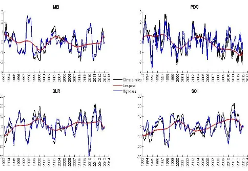
In order to investigate the climate variability of sea-level, we make use of four climate

indices (Figure 5). Figure 6 shows low-pass and high-pass filtered of these four climate

indices. The climate indices are low-pass filtered using consecutive application of a 25 and

37 months running mean and contain mainly variability at decadal and longer time scales

(Zhang et al., 1997, Vimont 2005). The corresponding high-pass filtered data are computed

by removing the low-pass-filtered data from the original data and contain mainly variability

1 2 3 4 5 6 7 8 9 10 11 12 13 14 15 16 17 18 19 20 21 22 23 24 25 26 27 28 29 30 31 32 33 34 35 36 37 38 39 40 41 42 43 44 45 46 47 48 49 50 51 52 53 54 55 56 57 58 59 60

with the low-passed SOI (correlation coefficient 0.88 at a 95% of the confidence interval in

Figure 6), which suggests a connection between the MJO and ENSO events at longer time

scales. This is consistent with the findings of Hendon et al. (2007), who found this

relationship by analysing variations in the sea surface temperature (SST), atmospheric winds

and convection in the Equatorial Pacific Ocean.

Table 2 lists correlations and lags between three Principal Components (PC) (time

series associated with first three EOFs) and four climate indices. Over 1993–2013, the first

principal component, PC1, highly correlated with MEI (-0.74, +1 month lag), high-passed

SOI (+0.65, 0 month lag) and high-passed OLR (+0.75, -1 month lag) (see also Figure 5).

The second principal component, PC2, has the largest amplitude along the north and east

coast and the largest correlation is with the MEI (+0.52, +5 month lag). The weak correlation

has been found for the third mode with OLR (-0.43, -8 month lag) above the 95% confidence

level. These results are consistent with the findings of White et al. (2014) showing that the

time series associated with the first EOF across whole Australia are highly correlated with the

SOI (+ 0.87 at 0 lag).

In brief, above results suggest a large part of the interannual sea-level fingerprint in

the northern Australian coastline shows a close connection to two climate events: ENSO and

MJO. The interannual transport is correlated with ENSO, there is a tendency for the eastward

flow of water from the Indian Ocean into the Pacific during El Niño events, which tends to

reverse during La Niña events. During El Niño events, westerly wind stress anomalies in the

central Pacific force eastward propagating equatorial Kelvin waves, depressing the

thermocline in the eastern Pacific cold tongue region (Zhang et al. 2006). These anomalous

wind force the westward spreading of Rossby waves, which lift the thermocline in the

western Pacific (Nidheesh et al. 2013). Rossby waves induce coastally trapped waves at the

1 2 3 4 5 6 7 8 9 10 11 12 13 14 15 16 17 18 19 20 21 22 23 24 25 26 27 28 29 30 31 32 33 34 35 36 37 38 39 40 41 42 43 44 45 46 47 48 49 50 51 52 53 54 55 56 57 58 59

north Australian and west Australian coasts. It has been also shown that the large annual

cycle in sea-level in the Gulf of Carpentaria and the Arafura Sea, is closely linked to the

monsoon. The transition from active to inactive phases of monsoon is connected to MJO.

There is also a connection between ENSO and MJO events. MJO affects the ENSO cycle and

can alter the evolution and intensity of El Niño and La Niña episodes.

4. Mean sea-level trend analysis using Mann-Kendall trend test

In the absence of absolute knowledge of mean sea-level, it is important that the trends are

tested to identify the most realistic value. The Mann-Kendall trend test (Mann 1945, Kendall

1975) is used in this study to assess the quality of computed trends from the harmonic

analysis (see section 3). The test was first introduced by Mann (1945) for the significance of

Kendall's tau where the X variable is time as a test for trend. The Mann-Kendall (M-K) test

can be defined most generally as a test for whether the trend to increase or decrease with time

(monotonic change). A monotonic upward (downward) trend means that the sea-level

consistently increases (decreases) through time within a specific level of significance. It

should be noted that the trend may or may not be linear. The M-K test examines whether to

reject the null hypothesis (H0: no monotonic trend) and accept the alternative hypothesis (H1:

the monotonic trend is present). The initial assumption of the M-K test is that the H0 is true

and that the data must be convincing beyond a reasonable doubt before H0 is rejected and H1

is accepted. The reader can refer to Pohlert (2015) for more details.

The focus is over a 20-year satellite altimetry period (1993 – 2013) using 14 tide

gauges to calculate trends (see Figure 1). Trends are derived at each altimetry along-track

points and tide gauges in the study area using the harmonic analysis method (cf. Equation 1

in section 3) after removing outliers based on the Pope test from datasets. The mean sea-level

1 2 3 4 5 6 7 8 9 10 11 12 13 14 15 16 17 18 19 20 21 22 23 24 25 26 27 28 29 30 31 32 33 34 35 36 37 38 39 40 41 42 43 44 45 46 47 48 49 50 51 52 53 54 55 56 57 58 59 60

identify the area in which trends are not monotonic or there is a discrepancy between

altimetry and tide gauge data sets especially closer to the coastline.

Linear trends from the satellite-altimeter data in the study region are shown in Figure

7. The rate of sea-level varies from ~2 mm/yr to ~13 mm/yr. The largest trends up to 13

mm/yr occurring around the northern part of Australia in the Gulf of Carpentaria and along

the Solomon Islands. The sea-level has been rising at the lowest rate along the east coast of

Australia between 20°S and 24°S, where the rates are generally ranging from about 1 mm/yr

(at about 24°S) up to 4 mm/yr. The rates of sea-level trends are slightly higher along the

Western Australia coastlines with magnitudes of more than 5 mm/yr, which may be

connected to the increasing sea surface temperature (SST) in this region (White et al. 2014).

Overall, the sea-level trends are similar for the deep ocean and coastal area, except for a few

stations as discussed above.

We applied the M-K trend test at the significant level α=0.05 on mean sea-level trends

obtained from both multi satellite altimeters observations with the aim of examining the

monotonic (upward or downward) trends in the study area. The results, as seen in Figure 8,

indicate that the majority of sea-level trends are monotonic (positive) over the study (red

regions in Figure 8) excluding the coastal area (distance to the coast <50 km) and some parts

of the Gulf of Carpentaria (blue regions). In the case of Gulf of Carpentaria, it is probably

due to the climate variability including El Niño/La Niña events along with a longer period

decadal change such as the Pacific Decadal Oscillation in this area. Another possible reason

could be the fact that this area is semi-enclosed seas of shallow depth, and is affected by the

strong ocean bottom pressure fluctuations. As expected, there are insignificant trends along

the coastlines where the geophysical corrections (e.g., ocean tides) cannot be estimated

accurately (Figure 8). Figure 9 illustrates an example of altimetry sea-level time series for a

1 2 3 4 5 6 7 8 9 10 11 12 13 14 15 16 17 18 19 20 21 22 23 24 25 26 27 28 29 30 31 32 33 34 35 36 37 38 39 40 41 42 43 44 45 46 47 48 49 50 51 52 53 54 55 56 57 58 59

contaminated by radar reflections from the land which can be improved by retracking

altimeter waveform data close to the coastline (Deng and Featherstone 2006). Jason-1 and

Jason-2 SSHs are now accurate within 5-10 km to the coast due to their ground retracking (or

reprocessing) procedure. However, retracked Topex data are not available, which can be

corrupted near the Australian coastline (Deng and Featherstone, 2002). From our analysis,

most near coastal trends that fail the test are resulted from inaccurate Topex data.

The comparison of trends is shown in Table 3, which presents the sea-level observed

at the closest along-track altimetry point to tide gauges with distances ~5-152 km. It can be

seen that altimetry and tide gauge data are highly correlated, showing a strong agreement

between trends of sea-level obtained from both data sets. In general, the rate of sea-level

trend is lower for offshore altimetry records than that from coastal tide gauge data, with a few

exceptions (e.g., Port Hedland and Wyndham). These differences are likely due to various

factors, such as differences in temperature and salinity, local winds, ocean currents as well as

local tectonic vertical movements (White et al. 2014). The largest difference has been found

at Honiara, where the rate of sea-level change estimated by altimetry ~65 km from the

coastline is considerably higher (11.8 mm/yr) than the coastal tide-gauge records (8.3

mm/yr). It is expected that the rate of coastal trend differs from the offshore rate at this

station as the SOLO-GPS near this station shows a negative trend

(http://www.sonel.org/spip.php?page=gps&idStation=2054 ). The highest rates of trends in

sea surface height are found around tide gauges located on the north and north-west of

Australia (e.g., Milner Bay, Wyndham). The rates of sea-level at these stations are ~9-10

mm/yr which is about three times faster than the rate of the global average sea-level trend

over this period. The rate of sea level at these stations can be related to VLM and tide gauge

stability. Burgette et al. (2013) found a positive VLM of 4.20 0.82 mm/yr at Wyndham tide

1 2 3 4 5 6 7 8 9 10 11 12 13 14 15 16 17 18 19 20 21 22 23 24 25 26 27 28 29 30 31 32 33 34 35 36 37 38 39 40 41 42 43 44 45 46 47 48 49 50 51 52 53 54 55 56 57 58 59 60

To further investigate the non-monotonic sea-level trends along the coastlines, the

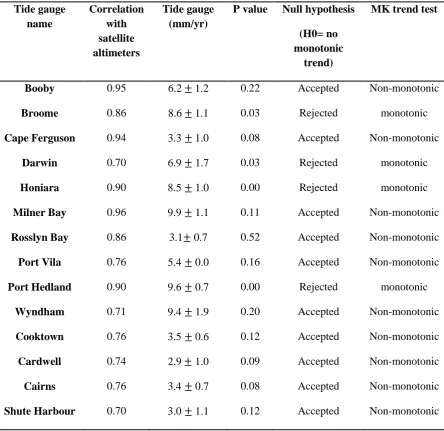
M-K test is performed on sea-level trends obtained from tide gauges observations. Table 4 lists

the M-K test results of sea-level trends from tide gauges in the study area. If the p value is

less than the significance level α (alpha) = 0.05, H0 is rejected. Rejecting H0 indicates that

there is a monotonic trend in the time series while accepting H0 indicates a non-monotonic

trend was detected. Insignificant trends (no monotonic trend, P value <0.05) are found for

tide gauges located along the north and north-east of Australia (e.g., tide gauge stations

Cairns and Booby), while trends are statistically significant at the north-west coastlines.

Along Australia’s north-east coast, the non-monotonic sea-level changes can be described by

the East Australian Current (EAC) that flows southward along the east coast and varies

considerably on interannual time scales (Bowen et al. 2005). Thus the sea-level in this area is

not rising steadily, in agreement with the results obtained from the M-K trend test. Based on

the above analysis, the sea-level trends from both altimetry and tide gauges are not

statistically significant in the Gulf Carpentaria which is largely affected by shallow water

tidal signals and natural climate variability (e.g., El Niño/La Niña).

These results indicate the need for caution in interpreting the previously reported

agreement of sea-level trends estimated by satellite altimetry and tide gauges data. For

example, Figure 10 shows a comparison of sea-level time series of Broome tide gauge station

and the closest satellite along–track normal point. Tide-gauge data are resampled by

averaging sea-level records within 3 hours around the time of altimeter along-track

measurements to generate compatible time series for both datasets. The datasets agree very

well with 86% correlation coefficient. While such agreement may indicate common

low-frequency behaviour in the data sets, it does not confirm the significance of trend estimates.

The large confidence intervals found from M-K test highlights the significant uncertainties

1 2 3 4 5 6 7 8 9 10 11 12 13 14 15 16 17 18 19 20 21 22 23 24 25 26 27 28 29 30 31 32 33 34 35 36 37 38 39 40 41 42 43 44 45 46 47 48 49 50 51 52 53 54 55 56 57 58 59

4.1. The basin-average sea-level from tide gauges and satellite altimetry

The altimetry-based sea-level has been averaged over the northern Australian coastline and

low-pass filtered using the moving average of 12 months (Figure 11). The low-pass filter is

used to remove high frequency components of sea-level. The altimetric sea-level trend over

1993–2013 indicates an overall rise of 6.1 0.3 mm/yr. The strong El Niño episodes

occurred during 1997-1998, causing a significant drop in the sea-level as can be seen in

Figure 11. The sea-level continues to rise again after two successive La Niña events (i.e.,

2007-2008 and 2008-2009) that reloaded the heat released by the 1997-1998 El Niño.

The basin average from tide gauge observations has been calculated by averaging the

sea-level data obtained from14 tide gauge stations over the study region. The combined tide

gauge time series has then been low-pass filtered to be comparable to the altimetric basin

average. The sea-level average over the study region from tide gauges and the altimeters

demonstrate a high correlation (0.9564), and small root mean squared errors (RMS, 18.0697

mm). This further confirms that there is a consistent agreement between offshore and coastal

sea-level variability around the northern Australian coastline. During 1993–2013, the rate of

sea-level trend recorded by tide gauges (6.3 0.4 mm/yr) is slightly higher than those

observed by satellite altimeters. In general, the average of tide gauge records follows a

similar pattern as compared to the corresponding altimetric data, the trend is positive before

2000, negative in 2000-2007 and positive afterwards.

5. Conclusion

Improvements in understanding the projection of sea-level rise require more knowledge of

regional sea-level changes. Here we focus on the northern part of Australia where climate

variability is larger, and the rate of sea-level rise is higher than the global average. This study

indicates that there is high coherence and correlation between the leading PCs of the sea-level

1 2 3 4 5 6 7 8 9 10 11 12 13 14 15 16 17 18 19 20 21 22 23 24 25 26 27 28 29 30 31 32 33 34 35 36 37 38 39 40 41 42 43 44 45 46 47 48 49 50 51 52 53 54 55 56 57 58 59 60

between a large part of sea-level fluctuations and the MJO and ENSO activities in this region.

Similarly, the highest annual sea-level variability (up to 30 cm, in the Gulf of Carpentaria)

has also been found during the tropical cyclone annual season, linking to the MJO which is

known to be a dominant deriver for tropical cyclone activity across this area.

Based on the average of sea-level over the whole study area, Sea-level change around

the northern Australian coastline indicates an overall rise of 6.3 ± 1.4 mm/yr and 6.1 ± 1.3

mm/yr from tide gauge and altimetry, respectively. The rate of sea-level change was

significantly higher than the global mean sea-level rise, which is likely associated with

periods of natural climate variability (e.g., MJO and ENSO). The variability in the north-east

of Australia is coherent and strongly correlated to the north-west of Australia suggesting that

sea-level changes in the Pacific and Indian oceans are connected through the Indonesian

throughflow (ITF).

For the period from 1993 to 2013, the estimated MSL trend rate from satellite

altimetry varies point by point but is generally in the range of -2 to 13 mm/year. The highest

rates of sea-level trend were observed around the north and north-west of Australia (up to 13

mm/yr) and the lowest rate (1-4 mm/yr) was found along the east coast of Australia,

consistent with previous findings in this region (e.g., White et al. 2014). In general, the rate of

the sea-level trend over the altimetry period was higher for offshore altimetry records than

that from coastal tide gauge data, with a few exceptions (e.g., Port Hedland and Wyndham).

The largest difference was found at Honiara, where the rate of sea-level change estimated by

altimetry ~65 km from the coastline was noticeably higher (11.8 mm/yr) than the coastal

tide-gauge records (8.3 mm/yr). This is possibly because of differences in temperature and

salinity, local winds, ocean currents and localised land movement.

Apart from the increasing rate of the sea-level, further investigation has been done to

1 2 3 4 5 6 7 8 9 10 11 12 13 14 15 16 17 18 19 20 21 22 23 24 25 26 27 28 29 30 31 32 33 34 35 36 37 38 39 40 41 42 43 44 45 46 47 48 49 50 51 52 53 54 55 56 57 58 59

trends (upward or downward). The results suggest that trends are statistically significant in

most of the region except along the north-east coasts and in the Gulf of Carpentaria due to the

effect of the natural variability and altimeter measurements are contaminated by the land. The

M-K trend test provides a more comprehensive description of regional sea-level variability

than the trend itself, allowing to quantify the monotonic mean sea-level trend.

In summary, we have introduced a novel framework for examining sea-level trends in

a future context, which has allowed us taking into account and removing the effect of

autocorrelations in different sea-level time series. This is of some significance in interpreting

of sea-level trends. Further research is required to improve the altimetry sea-level

measurement close to the coastline using retracking techniques. New altimetry missions, e.g.,

Jason-CS, Jason-3, CryoSat and Saral/AltiKa, should be included in future research.All these

new altimetry missions can significantly contribute to operational extreme sea-level

monitoring and forecasting. An improved understanding of sea-level rise will be helpful in

evaluating the coastal flooding scenario in the high flooding risk regions.

Acknowledgements

We would like to thank the anonymous reviewers and editors for their constructive comments on this article. We would like to acknowledge receipt of the Radar Altimeter Database System (RADS, http://rads.tudelft.nl/rads/rads.shtml) data team for kindly providing satellite altimetry data. The

1 2 3 4 5 6 7 8 9 10 11 12 13 14 15 16 17 18 19 20 21 22 23 24 25 26 27 28 29 30 31 32 33 34 35 36 37 38 39 40 41 42 43 44 45 46 47 48 49 50 51 52 53 54 55 56 57 58 59 60 References

Andersen, O. B. (1999). "Shallow water tides in the northwest European shelf region from TOPEX/POSEIDON altimetry." Journal of Geophysical Research: Oceans 104(C4): 7729-7741.

Andersen, O. B. and P. Knudsen (2009). "DNSC08 mean sea surface and mean dynamic topography models." Journal of Geophysical Research: Oceans (1978–2012) 114(C11).

Andersen, O.B., and R. Scharroo (2011). "Range and geophysical corrections in coastal regions: and implications for mean sea surface determination". In Coastal Altimetry, edited by S. Vignudelli, A. G. Kostianoy, P. Cipollini and J. Benveniste, pp.103-145, Berlin Springer, doi: 10.1007/978-3-642-12796-0.

Andersen, O. B, P. Knudsen, and L. Stenseng. (2015) "The DTU13 MSS (mean sea surface) and MDT (mean dynamic topography) from 20 years of satellite altimetry.": 1-10.

Barbosa, S. M., R. Scharroo and J. A. O. Matos (2012). Regional Sea-level Trends from Nearly 20 years of Radar Altimetry. 20 Years of Progress in Radar Altimetry.

Bureau of Meteorology,Birchip Cropping Group,Department of Agriculture, Fisheries and Forestry Bureau of Rural Sciences, Managing Climate variability, and Meat & Livestock Australia (2008). “Weather drivers in Queensland (Climate change fact sheets)”. Retrieved from

http://www.managingclimate.gov.au/wp-content/uploads/2010/12/1-QLD-weather-drivers_FINAL.pdf.

Bowen, M. M., J. L. Wilkin and W. J. Emery (2005). "Variability and forcing of the East Australian Current." Journal of Geophysical Research: Oceans (1978–2012) 110(C3).

1 2 3 4 5 6 7 8 9 10 11 12 13 14 15 16 17 18 19 20 21 22 23 24 25 26 27 28 29 30 31 32 33 34 35 36 37 38 39 40 41 42 43 44 45 46 47 48 49 50 51 52 53 54 55 56 57 58 59

Carrère, L., and F. Lyard (2003). "Modeling the barotropic response of the global ocean to atmospheric wind and pressure forcing‐comparisons with observations." Geophysical Research Letters 30(6): 1275, doi: 10.1029/2002GL016473

Cazenave, A., H.-B. Dieng, B. Meyssignac, K. von Schuckmann, B. Decharme and E. Berthier (2014). "The rate of sea-level rise." Nature Clim. Change 4(5): 358-361.

Cazenave, A. and R. S. Nerem (2004). "Present‐day sea-level change: Observations and causes." Reviews of Geophysics 42(3).

Cheng, Y. and O. B. Andersen (2011). "Multimission empirical ocean tide modeling for shallow waters and polar seas." Journal of Geophysical Research: Oceans (1978–2012) 116(C11). Church, J. and N. White (2011). "Sea-Level Rise from the Late 19th to the Early 21st Century."

Surveys in Geophysics 32(4-5): 585-602.

Church, J. A., P. U. Clark, A. Cazenave, J. M. Gregory, S. Jevrejeva, A. Levermann, M. Merrifield, G. Milne, R. Nerem and P. Nunn (2013). "Sea-level change." Climate change: 1137-1216. Church, J. A., J. R. Hunter, K. L. McInnes and N. J. White (2006). "Sea-level rise around the

Australian coastline and the changing frequency of extreme sea-level events." Australian Meteorological Magazine 55(4): 253-260.

Church, J. A. and N. J. White (2006). "A 20th century acceleration in global sea-level rise." Geophysical Research Letters 33(1): n/a-n/a.

Deng, X. and W. Featherstone (2006). "A coastal retracking system for satellite radar altimeter waveforms: Application to ERS‐2 around Australia." Journal of Geophysical Research: Oceans (1978–2012) 111(C6).

Deng, X., Z. Gharineiat, O. Andersen and M. Stewart (2015). Observing and Modelling the High Water Level from Satellite Radar Altimetry During Tropical Cyclones, Springer Berlin Heidelberg: 1-9.

1 2 3 4 5 6 7 8 9 10 11 12 13 14 15 16 17 18 19 20 21 22 23 24 25 26 27 28 29 30 31 32 33 34 35 36 37 38 39 40 41 42 43 44 45 46 47 48 49 50 51 52 53 54 55 56 57 58 59 60

Dorandeu, J. and P. Y. Le Traon (1999). "Effects of Global Mean Atmospheric Pressure Variations on Mean Sea-level Changes from TOPEX/Poseidon." Journal of Atmospheric and Oceanic Technology 16(9): 1279-1283.

Fasullo, J. T., C. Boening, F. W. Landerer and R. S. Nerem (2013). "Australia's unique influence on global sea-level in 2010–2011." Geophysical Research Letters 40(16): 4368-4373.

Gharineiat, Z. and X. Deng (2015). "Application of the Multi-Adaptive Regression Splines to Integrate Sea-level Data from Altimetry and Tide Gauges for Monitoring Extreme Sea-level Events." Marine Geodesy 38(3): 261-276.

Haigh, I., M. Eliot, C. Pattiaratchi and T. Wahl (2011). "Regional changes in mean sea-level around Western Australia between 1897 and 2008."

Hall, J. D., A. J. Matthews and D. J. Karoly (2001). "The modulation of tropical cyclone activity in the Australian region by the Madden-Julian Oscillation." Monthly Weather Review 129(12): 2970-2982.

Hendon, H. H., C. Zhang and J. D. Glick (1999). "Interannual variation of the Madden-Julian oscillation during austral summer." Journal of Climate 12(8): 2538-2550.

Idris, N. H., X. Deng and O. B. Andersen (2014). "The importance of coastal altimetry retracking and detiding: a case study around the Great Barrier Reef, Australia." International Journal of Remote Sensing 35(5).

Kendall, M. (1975). "Rank Correlation Methods (Charles Griffin, London, 1975)."

Lambert, A. (1974). "Earth tide analysis and prediction by the response method." Journal of Geophysical Research 79(32): 4952-4960.

Lavender, S. L. and A. J. Matthews (2009). "Response of the West African monsoon to the Madden-Julian oscillation." Journal of Climate 22(15): 4097-4116.

Madden, R. A. and P. R. Julian (1972). "Description of global-scale circulation cells in the tropics with a 40-50 day period." Journal of the Atmospheric Sciences 29(6): 1109-1123.

1 2 3 4 5 6 7 8 9 10 11 12 13 14 15 16 17 18 19 20 21 22 23 24 25 26 27 28 29 30 31 32 33 34 35 36 37 38 39 40 41 42 43 44 45 46 47 48 49 50 51 52 53 54 55 56 57 58 59

Mantua, N. J. and S. R. Hare (2002). "The Pacific decadal oscillation." Journal of oceanography 58(1): 35-44.

Mantua, N. J., S. R. Hare, Y. Zhang, J. M. Wallace and R. C. Francis (1997). "A Pacific interdecadal climate oscillation with impacts on salmon production." Bulletin of the american Meteorological Society 78(6): 1069-1079.

Marshall, A. and H. Hendon (2014). "Impacts of the MJO in the Indian Ocean and on the Western Australian coast." Climate dynamics 42(3-4): 579-595.

Maul, G.A. and D.M. Martin (1993). "Sea-level rise at key west, Florida, 1846–1992: America’s longest instrument record?". Geophysical Research Letters. 20 (18): 1955– 1958.

Meyssignac, B. and A. Cazenave (2012). "Sea-level: A review of present-day and recent-past changes and variability." Journal of Geodynamics 58: 96-109.

Nerem, R. S., E. Leuliette and A. Cazenave (2006). "Present-day sea-level change: A review." Comptes Rendus Geoscience 338(14): 1077-1083.

Nidheesh, A. G., Lengaigne, M., Vialard, J., Unnikrishnan, A. S., & Dayan, H. (2013). "Decadal and long-term sea-level variability in the tropical Indo-Pacific Ocean. " Climate dynamics 41(2): 381-402.

Parker, R. L. (1994). Geophysical inverse theory, Princeton university press.

Pohlert, T. (2015). "trend: Non-Parametric Trend Tests and Change-Point Detection". http://CRAN.R-project.org/package=trend

Peltier, W. (2004). "Global glacial isostasy and the surface of the ice-age Earth: the ICE-5G (VM2) model and GRACE." Annu. Rev. Earth Planet. Sci. 32: 111-149.

Pope, A. J. (1976). "The statistics of residuals and the detection of outliers."

Rahmstorf, S., A. Cazenave, J. A. Church, J. E. Hansen, R. F. Keeling, D. E. Parker and R. C. Somerville (2007). "Recent climate observations compared to projections." Science 316(5825): 709-709.

1 2 3 4 5 6 7 8 9 10 11 12 13 14 15 16 17 18 19 20 21 22 23 24 25 26 27 28 29 30 31 32 33 34 35 36 37 38 39 40 41 42 43 44 45 46 47 48 49 50 51 52 53 54 55 56 57 58 59 60

Scharroo, R. and W. H. F Smith (2010). "A global positioning system–based climatology for the total electron content in the ionosphere." Journal of Geophysical Research: Space Physics 115(A10), doi: 10.1029/2009JA014719.

Tamisiea, M. E. (2011). "Ongoing glacial isostatic contributions to observations of sea-level change. " Geophysical Journal International 186(3): 1036-1044.

Ventrice, M. J., M. C. Wheeler, H. H. Hendon, C. J. Schreck III, C. D. Thorncroft and G. N. Kiladis (2013). "A modified multivariate Madden–Julian oscillation index using velocity potential." Monthly Weather Review 141(12): 4197-4210.

Vimont, D. J. (2005). "The contribution of the interannual ENSO cycle to the spatial pattern of decadal ENSO-like variability. " Journal of climate 18: 2080–2092.

Wahl, Thomas, I. D. Haigh, Philip L. Woodworth, F. Albrecht, D. Dillingh, Jürgen Jensen, Robert J. Nicholls, Robert Weisse, and G. Wöppelmann (2013). " Observed mean sea-level changes around the North Sea coastline from 1800 to present. " Earth-Science Reviews.124: 51-67. Wahl, Thomas, Jürgen Jensen, Torsten Frank, and Ivan David Haigh (2011). "Improved estimates of

mean sea-level changes in the German Bight over the last 166 years." Ocean Dynamics . 61(5): 701-715.

Walker, G. T. (1923). "Correlation in seasonal variations of weather VIII." Mem. India Meteor. Dept 24: 75-131.

Watson, C. S., N. J. White, J. A. Church, M. A. King, R. J. Burgette and B. Legresy (2015). "Unabated global mean sea-level rise over the satellite altimeter era." Nature Clim. Change 5(6): 565-568.

Watson, P. J. (2016). "Acceleration in U.S. Mean Sea-level? A New Insight using Improved Tools." Journal of Coastal Research 32(6):1247-1261.

1 2 3 4 5 6 7 8 9 10 11 12 13 14 15 16 17 18 19 20 21 22 23 24 25 26 27 28 29 30 31 32 33 34 35 36 37 38 39 40 41 42 43 44 45 46 47 48 49 50 51 52 53 54 55 56 57 58 59

Wheeler, M. C. and H. H. Hendon (2004). "An All-Season Real-Time Multivariate MJO Index: Development of an Index for Monitoring and Prediction." Monthly Weather Review 132(8): 1917-1932.

White, N. J., I. D. Haigh, J. A. Church, T. Koen, C. S. Watson, T. R. Pritchard, P. J. Watson, R. J. Burgette, K. L. McInnes, Z.-J. You, X. Zhang and P. Tregoning (2014). "Australian sea-levels—Trends, regional variability and influencing factors." Earth-Science Reviews 136: 155-174.

Woodworth, P. L., Teferle, F. N., Bingley, R. M., Shennan, I., & Williams, S. D. P. (2009). " Trends in UK mean sea-level revisited. " Geophysical Journal International. 176(1): 19-30.

Wolter, K. (1989). "Modes of tropical circulation, Southern Oscillation, and Sahel rainfall anomalies." Journal of climate 2(2): 149-172.

Zhang, X. and J. A. Church (2012). "Sea-level trends, interannual and decadal variability in the Pacific Ocean." Geophysical Research Letters 39(21).

Zhang, Xuebin, and Michael J. McPhaden (2006). "Wind stress variations and interannual sea surface temperature anomalies in the eastern equatorial Pacific." Journal of climate 19 (2) : 226-241. Zhang, Y., J. M. Wallace, and D. S. Battisti (1997). "ENSO-like interdecadal variability: 1900–

Table 1. Summary of the standard range and geophysical corrections selected from the

RADS database, as applied in this study.

Correction Available through RADS at

the time of this study

Selected for this research

Correction (m)

min max

Dry tropospheric NCEP/NCAR model ECMWF model

ECMWF model -2.4 +2.1

Wet tropospheric radiometer measurement ECMWF model

NCEP/NCAR model NASA NVAP model TOVS/SSMI data TOVS/NCEP hybrid

ECMWF model -0.6 +0.05

Ionosphere Smoothed dual-frequency

DORIS model CODE GIM model JPL GIM model

Smoothed dual-frequency altimeter

-0.4 +0.04

Tides

(include long-period a load tides)

GOT4.9 model FES2012 model

With consistent pole and solid Earth tides

Response method -5 +5

Sea state bias BM3/BM4 model

CLS non-parametric model CSR-A/B model hybrid model

BM4 model -1 +1

Geoid/mean sea surface (MSS)

CLS01 MSS model CNES-CLS11 MSS model EGM2008

(geoid and MSS) DTU13 MSS model

DTU13 MSS model

(Andersen et al. 2015)

-200 +200

Dynamic atmosphere

IB (model, local pressure) MOG2D_IB model

Table 2. Correlations and their associated lags between the first three PC components (e.g.,

PC1, PC2 and PC3) and the climate indices. A positive lag indicates that the index is later

than PC 1. SOI and OLR index has been high-pass filtered.

Principle component

MEI SOI OLR PDO

PC1 Correlation -0.74 +0.65 +0.75 -0.47

Lag(months) +1 0 -1 +1

PC2 Correlation +0.52 +0.34 -0.33 -0.31

Lag(months) +5 +22 -22 -14

PC3 Correlation -0.36 +0.35 -0.43 -0.26

Table 3. Linear trend (mm/yr) between 1993 and 2013 from both tide gauge and satellite

altimetry data at closest along-track points to 14 tide gauge stations. Note that hourly tide

gauge data has been resampled ± 3 hours around the time of altimetry data.

Tide gauge Correlation Distance (km) Resampled

Tide gauge (mm/yr)

Satellite (mm/yr)

Booby 0.95 5.6 6.2 1.2 9.5 1.2

Broome 0.86 28.9 8.4 1.1 8.1 0.0

Cape Ferguson 0.93 53.0 3.1 1.0 4.5 0.9

Darwin 0.70 138.4 6.6 1.7 7.0 1.1

Honiara 0.90 65.3 8.3 1.0 11.8 0.0

Milner Bay 0.96 96.8 9.7 1.1 9.8 1.1

Rosslyn Bay 0.85 79.4 2.8 0.7 3.7 0.7

Port Vila 0.75 80.9 5.3 0.0 6.1 0.0

Port Hedland 0.90 78.1 9.3 0.7 7.2 0.6

Wyndham 0.71 107.7 9.1 1.9 8.7 0.9

Cooktown 0.76 56.5 3.2 0.6 5.5 0.5

Cardwell 0.74 92.2 2.9 1.0 4.0 0.8

Cairns 0.76 218.9 3.1 0.7 6.7 0.6

Table 4. The results of the Mann-Kendall trend test at the significance level α=0.05 for the

tide gauges located around the northern Australian coastlines for the period of 1993-2013.

Tide gauge name

Correlation with satellite altimeters

Tide gauge (mm/yr)

P value Null hypothesis (H0= no monotonic

trend)

MK trend test

Booby 0.95 6.2 1.2 0.22 Accepted Non-monotonic

Broome 0.86 8.6 1.1 0.03 Rejected monotonic

Cape Ferguson 0.94 3.3 1.0 0.08 Accepted Non-monotonic

Darwin 0.70 6.9 1.7 0.03 Rejected monotonic

Honiara 0.90 8.5 1.0 0.00 Rejected monotonic

Milner Bay 0.96 9.9 1.1 0.11 Accepted Non-monotonic

Rosslyn Bay 0.86 3.1 0.7 0.52 Accepted Non-monotonic

Port Vila 0.76 5.4 0.0 0.16 Accepted Non-monotonic

Port Hedland 0.90 9.6 0.7 0.00 Rejected monotonic

Wyndham 0.71 9.4 1.9 0.20 Accepted Non-monotonic

Cooktown 0.76 3.5 0.6 0.12 Accepted Non-monotonic

Cardwell 0.74 2.9 1.0 0.09 Accepted Non-monotonic

Cairns 0.76 3.4 0.7 0.08 Accepted Non-monotonic

Figure 1. The distribution of satellite altimeter ground tracks and the location of tide gauges

(green stars) used for analysing regional sea level variability and trends between 1993 and

Figure 2. Amplitudes (in mm) of annual (top) and semi-annual (bottom) sea level signals for

Figure 3. Principles components (PCs) of three leading modes of EOF represent temporal

Figure 4. The spatial distributions of the first three EOF modes are computed from the

multi-mission satellite altimeter TOPEX, Jason 1 and Jason 2 data over the northern Australian

coastlines. The top panel shows EOF1 (44.6% variance), the middle panel shows EOF2

Figure 5. The Principal Component (PC) of the first EOF mode plotted against three climate

indices. It should be noted that the magnitudes of MEI and OLR are enlarged by 10 times for

Figure 6. The four climate indices (black) used in this study along with their low-pass

filtered (red) and high-pass filtered (blue) components. The climate indices are the

Multivariate Enso Index (MEI), Pacific Decadal Oscilation (PDO), Outgoing Longwave

Figure 7. Sea level trend (mm/yr) calculated from multi-missions satellite altimeters between

Figure 8. Map of Mann-Kendall test results at the significance level α=0.05 on sea level

trends obtained from satellite altimetry. Red represents the area in which sea levels have an

upward or a downward trend and blue represents the area where there are no monotonic

Figure 9. An example of satellite altimetry sea level time series for a point located ~55 km

Figure 10. Comparisons of tide-gauge and satellite-altimeter data. Top panel: Satellite

altimeter data at the closest along-track normal point to Broome station (122°7′55″ E,

17°45′43″S). Middle panel: Hourly tide gauge data at Broome station (121°49′4″ E,

18°0′3″S). Bottom panel: Tide gauge data are resampled around satellite altimeter data.

Tide-gauge data is plotted in red, satellite altimeter data in blue and the correlation between the

Figure 11. Basin average of sea level around the northern Australian coastline from altimetry

(circle) and from tide gauges (triangle). 14 tide gauge stations (green stars in Figure 1) have

been used to calculate the basin-average. A 12-month moving average has been applied to the

Response to Review Comments

(Manuscript Number: TRES-PAP-2016-0404)

We would like to thank the editor and all reviewers for their constructive comments on the

manuscript, which helped us to improve the work. We hope our revision has improved the

paper to a level of their satisfaction. Number wise answers to their specific comments are as

follows.

Response to Reviewer #1 Comments

Thank-you for the opportunity to review Dr Gharineiat and Dr Deng's revised paper. Having

considered the responses to the prior review comments, I'm satisfied that all necessary

clarifications, revisions and concerns that I raised have now been adequately addressed by the

authors. Thank-you again for the opportunity to consider the revised manuscript.

Response: We sincerely thank both reviewers for their careful reading of our manuscript and

their insightful comments and suggestions.

Response to Reviewer #2 Comments

The quality of the paper has improved quite well and is now almost ready for acceptance. The

attached PDF is annotated with some minor typos corrected.

Response: We sincerely thank both reviewers for their careful reading of our manuscript and

their insightful comments and suggestions.

All typos are corrected in the revised manuscript. We also corrected Port Vila and Shute

Harbour in all figures.

Comment 1: Page 11, line 8: Did you work on 10 day or on the exact TP/J1/J2/J3 repeat

period (9.9156 days)?

Response: We used the exact TP/J1/J2/ repeat period. It is corrected in the revised

manuscript.

Comment 2: Page 12, line 7 onward

You are now mention explicitly on page 6 the use of 1Hz along-track altimetry data for

construction Figure 1, trying to prevent interpolation errors. For all figures starting with

Figure 4 it seems you have used interpolated grids. This would contradict your attempt to *Detailed Response to Reviewers