Modelling techniques for structural evaluation for bridge assessment

Modelling Techniques for Structural Evaluation for Bridge Assessment

2

Shojaeddin Jamali

, Tommy H.T. Chan

, Andy Nguyen

and David P. Thambiratnam

4

1_{Shojaeddin Jamali, Department of Civil Engineering and Built Environment, Queensland University of} 5

Technology. Email: [email protected], orcid.org/0000-0001-7381-8522 6

7

2_{Corresponding author, Tommy Chan, Department of Civil Engineering and Built Environment, Queensland} 8

University of Technology. Email: [email protected], orcid.org/0000-0002-5410-8362 9

10

3_{Andy Nguyen, Department of Civil Engineering and Built Environment, Queensland University of Technology.} 11

Email: [email protected], orcid.org/0000-0001-8739-8207 12

13

4_{David Thambiratnam, Department of Civil Engineering and Built Environment, Queensland University of} 14

Technology. Email: [email protected], orcid.org/0000-0001-8486-5236 15

16

Abstract 17

Load assessment of existing bridges in Australia is evaluated mainly using beam line model and the grillage 18

analogy to examine the structural integrity of bridge components due to live loadings. With the majority of existing 19

bridge networks designed for superseded design vehicular loading, the necessity to utilise more rigorous analysis 20

methods to assess the load effects of bridges is indispensable. In this paper, various vehicular loading cases on a 21

grillage model of a box girder bridge and its equivalent finite element model (FE) are considered, and their 22

applicability for bridge assessment using structural health monitoring (SHM) as defined in the new revision of AS 23

5100.7 is studied. Based on numerical analyses, it was observed that component-level load effects in the two 24

models have notable differences, irrespective of vehicle speed, position and loading. However, when global-level 25

load responses are compared, the discrepancy in analysis outputs drops dramatically. The modelling ratios 26

developed in this paper are practical and will be applicable with any modelling techniques for bridge assessment 27

under vehicular loading on both a global and component-response basis. It was also observed that FE is more 28

efficient in terms of model updating and damage simulation, and hence more appropriate for implementation of 29

SHM techniques. The proposed flowchart suggested for heavy load assessment incorporates detailed and simple 30

modelling approaches aligned with experimental data obtained by SHM techniques, which can be used for 31

periodic and long term monitoring of bridges. It can enhance the proper determination of bridge condition states, 32

as any conservative estimation of bridge capacity may result in unnecessary load limitations. 33

Keywords: Bridge assessment, grillage analogy, finite element model, load assessment, structural health 34

1.

Introduction

Enormous developments in technology have occurred since the introduction of the first hand-held calculator 2

in 1970 [1]. This advancement of technology had a revolutionary impact on engineering applications, owing to 3

the fact that nowadays computer modelling has become an indivisible part of engineering design and analysis. 4

Prevalent use of computer modelling has assisted civil engineers to effectively analyse structures both in pre-5

design and post-design stages [2]. When it comes to a computerised approach, a trade-off between speed of 6

analysis, complexity of model and degree of accuracy always exist. For the purpose of bridge design, finite 7

element (FE) analysis and grillage analogy (GA) have remained as valuable methods. In GA, the bridge 8

superstructure is modelled by equivalent longitudinal and transverse beams, while FE analysis discretises the deck 9

into different elements connected together based on equilibrium and/or compatibility conditions. In short, a 10

structural system matrix in GA is formed using a usual stiffness matrix approach as in the FE method. In the 11

authors’ previous publication, the FE model was coupled with modal analysis techniques to assess the structural 12

condition of an overpass [3]. GA idealises the bridge as series of discrete longitudinal and transverse beam 13

elements connected by nodal points. Jaeger and Bakht [4] state the widespread use of grillage model to be a 14

simplification of bridge components that can represent its complicated features to carry out necessary design 15

calculations. A number of previous researchers used GA in their post-design stage as well. Lu et al. [5] validated 16

the grillage model of a T-frame bridge using results obtained from field testing. Sadeghi and Fathali [6] compared 17

vibration parameters of a grillage theoretical model with the experimental data and concluded that GA has a 18

satisfactory degree of accuracy when the bridge loads do not exceed the allowable amount. Also, other similar 19

studies collated grillage results with field testing data for bridge assessment [7-9]. 20

The design vehicle loading of SM1600 is used for new bridges in Australia, though, more than half of existing 21

bridge networks were designed based on the T44 design loading [3]. In addition to bridge design, GA is also used 22

in Australia for bridge load assessment according to the guidelines outlined in Transport and Main Road (TMR) 23

[10] and AS5100.7 [11]. A recently released version of AS 5100.7 [12] includes an introduction to road and rail 24

assessment vehicles, fatigue assessment, improved load factors, rating equations for combined actions and 25

addition of structural health monitoring (SHM) as bridge assessment approaches. In this standard, SHM is defined 26

as “the use of various sensing devices and ancillary systems to monitor the in situ behaviour of a structure to 27

condition testing, damage detection and assessment, system identification and performance monitoring are 1

provided. 2

This major transition in the national bridge code implies the need for more rigorous analysis for assessment 3

of aged bridges, which have been pillars of economic growth in Australia [13,14]. Therefore, any modelling 4

techniques used for bridge structural assessment must be able to demonstrate the realistic structural response of 5

the bridges. Based on the best knowledge of the present authors, there has been no officially published work on 6

application of GA for bridge heavy load assessment. Idealisation of bridges by grillage is not axiomatic and it has 7

pitfalls. Output of GA requires interpretations and cannot be applied directly to the structure [15]. Also, only 8

vertical loads (concentrated or line loads) could be directly applied [16]. Effect of construction sequence, 9

reinforcement modelling, analysis of secondary effects, in-plane effects and nonlinear response of deck are a few 10

other limitations of GA which are neglected in the modelling [17,18]. These downsides of GA makes it a weak 11

solution for comprehensive bridge assessment, which differs entirely from design philosophy. This paper 12

evaluates the effectiveness of GA and FE in bridge load assessment by providing numerical investigation on a 13

prestressed concrete box girder bridge. Different static and moving loads are considered to examine the 14

performance of modelling techniques, and to study the applicability of SHM for bridge load assessment with 15

respect to new AS 5100.7. 16

2.

Modelling approach

The bridge of interest in this study is a simply supported 30m single span, three cellular bridge deck with edge 18

cantilevers and solid diaphragms at supports, which is a typical bridge deck and span length currently open to 19

traffic in Queensland State of Australia. No special features like heavy skew and sloped web are considered to 20

generalise the analysis in the bridge profiles. A rendered view of FE and grillage models are shown in Figure 1. 21

Fig. 1 Finite element and grillage models of box girder (modelled in CSiBridge software) 22

23

Unlike the FE method, which incorporates 6 Degrees of Freedom (DOF), GA only has 3 DOF known as 24

rotation about planar axes and displacement in a vertical direction. In GA, the main concept lies in working out 25

the mesh grid and sectional properties of the beam elements. The deck is idealised into equivalent grillage by 26

using web-based division, whereby the longitudinal members coincide with lines of strength in girders and 27

needed to ensure proper distribution of loads. Gridlines are normally taken at right angles with similar spacing in 1

both directions. Typically, spacing of transverse members is more than that in the longitudinal direction since 2

transverse members have relatively smaller moment capacity [19,18]. Thus, spacing ratio of transverse to 3

longitudinal members is taken as1:1.11. 4

For exterior and interior longitudinal girders, the 2nd _{moment of area is taken about the centroid of physical} 5

girders, including portions of slab, whereas for transverse members the tributary area for the 2nd _{moment of area} 6

is with respect to top and soffit slabs. It is very important not to overcompensate for the weight of the deck slab 7

in computations of transverse members, since weight is already considered in longitudinal directions. In order to 8

reproduce the distortional behaviour of cells in both directions, a shear flexible grillage model is adopted. 9

Following AS 5100.5, the effect of shear lag is found to be insignificant in this modelling [20]. Torsional stiffness 10

of longitudinal and transverse members is computed following the procedures outlined by Hambly [15]. For 11

constructing the finite element model of box girder, shell elements were used with material and sectional 12

properties from design drawings. Each shell element is formulated based on Kirchhoff plate theory [21] and has 13

6 DOF, which means both in-plane and out-of-plane deformation is considered (combination of membrane and 14

plate behaviours). In the FE model, interaction of web with top and soffit slabs is considered integral by creating 15

a series of nodal restraints that are interconnected. A mesh convergence study was conducted to find a suitable 16

mesh size for the FE model considering accuracy and computational time. Recommendations for FE modelling 17

techniques and updating are described elsewhere [3,22]. Further reading on computer modelling of bridges using 18

GA are also available in the literature [23,19,18]. 19

3.

Arrangement of loadings

Referring to Figure 1, two-lane box girder is loaded for transient load analysis considering standard design 21

lane of 3.1m. Moving loads were discretised by an increment of 1% span length to achieve higher accuracy. Before 22

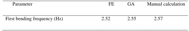
applying any external loading, soundness of both models statically and dynamically were checked (see Table 1) 23

by comparing total dead load and fundamental frequency with results of manual calculation. 24

Table 1. Comparison of GA, FE models and manual calculations 25

Parameter FE GA Manual calculation

Total max momentunder gravity load (kN.m) 8825.3 8876.3 8848.8

1

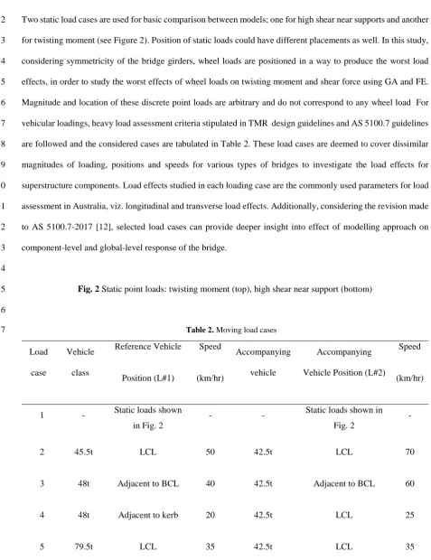
Two static load cases are used for basic comparison between models; one for high shear near supports and another 2

for twisting moment (see Figure 2). Position of static loads could have different placements as well. In this study, 3

considering symmetricity of the bridge girders, wheel loads are positioned in a way to produce the worst load 4

effects, in order to study the worst effects of wheel loads on twisting moment and shear force using GA and FE. 5

Magnitude and location of these discrete point loads are arbitrary and do not correspond to any wheel load For 6

vehicular loadings, heavy load assessment criteria stipulated in TMR design guidelines and AS 5100.7 guidelines 7

are followed and the considered cases are tabulated in Table 2. These load cases are deemed to cover dissimilar 8

magnitudes of loading, positions and speeds for various types of bridges to investigate the load effects for 9

superstructure components. Load effects studied in each loading case are the commonly used parameters for load 10

assessment in Australia, viz. longitudinal and transverse load effects. Additionally, considering the revision made 11

to AS 5100.7-2017 [12], selected load cases can provide deeper insight into effect of modelling approach on 12

component-level and global-level response of the bridge. 13

14

Fig. 2 Static point loads: twisting moment (top), high shear near support (bottom) 15

16

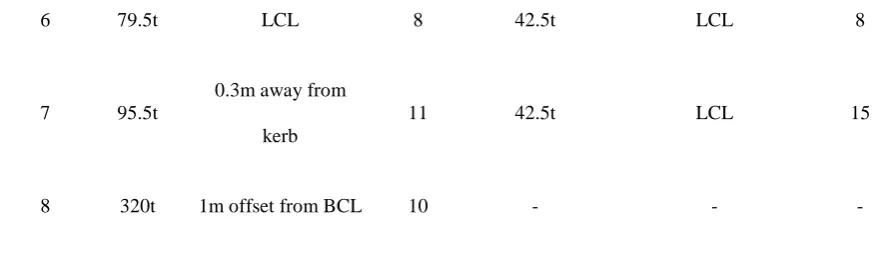
Table 2. Moving load cases

17

Load case

Vehicle class

Reference Vehicle

Position (L#1)

Speed

(km/hr)

Accompanying vehicle

Accompanying Vehicle Position (L#2)

Speed

(km/hr)

1 - Static loads shown

in Fig. 2

- - Static loads shown in

Fig. 2

-

2 45.5t LCL 50 42.5t LCL 70

3 48t Adjacent to BCL 40 42.5t Adjacent to BCL 60

4 48t Adjacent to kerb 20 42.5t LCL 25

Note: LCL= lane centreline, BCL= bridge centreline, L# = lane number, kerb= measured from outer face of wheel

1

4.

Discussion of analysis

Results of numerical analyses are detailed in the next sections. Only results of specific elements are compared 3

for each load case in both models for the sake of brevity. For each load effect, the response of the bridge before 4

and after point of interest was averaged to improve accuracy. 5

4.1. Load case 1: static wheel loads 6

The results of static point loads are set out in Figure 3. The effects of point loads near supports in GA are 7

similar to those of FE. Induced high shear load is shown as a sharp change in the diagram for G3; while G2 8

received less intensity of load. In contrast, GA underestimated the twisting moment caused by antisymmetric 9

point loads. In GA, high torsional stiffness of cells are reproduced by allocating high torsion constants to 10

longitudinal and transverse elements. When cellular decks are subjected to twisting action, shear flow passes 11

through slabs and webs. In GA, total torque is made up partly from shear forces on sides of the deck and from 12

opposed torques in longitudinal members, and the torque in transverse members are in equilibrium with the shear 13

forces in slab perimeter. One reason that GA misidentified the torque is that the postulated sum of torsion constant 14

in longitudinal members is equal to half of the torsion stiffness of the deck when treated as a beam, which means 15

that longitudinal members only provide half of the torque imposed on cross section; whereby the other half is 16

provided by shear forces flowing on the sides of the deck. Consequently, when the deck is loaded by asymmetric 17

position and different quantity of torque, the relationship between beam torsional constant and slab is no longer 18

related. Also, it is likely that this non-uniform twisting movement causes the shear flow in the slab perimeter and 19

webs to flex out of plane independently. On the other hand, FE simulates the torsion behaviour of girders by 20

identifying a lesser quantity of torsional deformation for G2 and G3, respectively. 21

Fig. 3 Shear diagram (left) and torsion diagram (right) 22

6 79.5t LCL 8 42.5t LCL 8

7 95.5t

0.3m away from kerb

11 42.5t LCL 15

1

2

4.2. Load case 2: longitudinal bending moment 3

Figure 4 illustrates the longitudinal bending moments of interior and exterior girder due to moving loads. It 4

can be seen that GA reported a very close moment profile to that of FE for G2 and G4. There is some loss of 5

accuracy in initial and end support conditions for minimum bending moment that remained undetected in GA due 6

to the restrained 3DOF. Also, slightly lesser bending moment output by FE for G4 can be attributed to the fact 7

that FE normally gives stiffer transverse distribution, which is due to composite interaction of slab with closed-8

box section of each cell [18]. In GA, the moment diagram has a sawtooth shape with sharp jumps at nodal points, 9

which is due to the transition of torsion in transverse members to shear and bending in the longitudinal direction. 10

It is assumed that the true structural moment diagram can be taken as the average of those on either side of each 11

joint. Division of longitudinal members is a key factor in simulating the longitudinal bending of the cellular deck. 12

Resistance to external loading is provided by top and bottom slabs, which causes the girders to flex about a 13

common axis. 14

15

Fig. 4 Longitudinal bending moment profile 16

17

4.3. Load case 3: longitudinal shear force 18

Longitudinal shear profile due to two truck loadings adjacent to BCL is presented in Figure 5. The comparison 19

is made for left exterior and second interior girders. Shear distribution in GA is similar to that of FE, only a small 20

difference is observed in supports. This difference is caused by degree of fixity of support conditions, because in 21

the FE model in addition to local and global effects, in-plane effects (in this case shear in planar directions) is also 22

taken into account. This can give rise to a pinned support behaves in semi-fixed condition since all DOF are 23

considered in analysis. Output of shear force in GA is the slope of the true structural moment diagram. Total shear 24

force for design of the webs is the combination of shear force due to bending and due to torsion, since torsional 25

shear force of girders (longitudinal members) stems from equivalent torsion of transverse members. Low shear 26

stiffness was given to grillage members to match the deformation of the cellular deck when subjected to equal 27

proportional to shear force; whereas, in cellular decks, shear force is also dependant on the continuity of concave 1

moments of slabs in adjacent cells. 2

3

Fig. 5 Longitudinal shear force profile 4

5

4.4. Load cases 4 and 5: dynamic analysis 6

Dynamic displacement and acceleration of exterior girders were recorded in both models by using time history 7

analysis, which is displayed in Figure 6. A gridline of GA was drawn on the FE model to have similar nodes on 8

deck for measurements. For load case 3, vertical accelerations in both models were measured at nodal points 9

corresponding to 6m of girder length from left support. GA had a sharp drop in detecting all peak values and 10

downgraded the acceleration, though the trend of measurement is comparable to that of FE. It should be noted it 11

is impractical to have the sensors on the deck due to traffic interruption. In the FE model, the response at various 12

locations along the girder length, such as bottom or midway of web can be obtained; while in GA, only nodal 13

points connecting the members can be considered as measurement locations. 14

Fig. 6 Acceleration (top) and displacement (bottom) of exterior girders 15

16 17

For load case 4, deflection at mid-span of deck was measured. Since the spacing of transverse members was set 18

to 2m, additional nodal points in the grillage model had to be configured to capture the midspan displacement. 19

Figure 6 shows that there has been a gradual increase in estimation of displacement by GA. This difference can 20

be explained by the fact that in GA, the deflection of longitudinal members are merely reported; while in FE, the 21

deflection of girders is a result of interaction between slabs and webs. This may lead to different load distributions 22

and in turn to lesser deflections. Another important aspect to consider when assessing the dynamic behaviour of 23

bridges is to include the existing conditions. Although it is possible to change the material properties and support 24

conditions of grillage members to some extent by introducing very fine mesh, GA is incapable of modelling 25

diverse damage types that might happen throughout the life of the structure. These two load cases were considered 26

to see how the SHM concept can be embedded in modelling techniques for the purpose of load assessment. 27

Compared with the FE method, GA is more challenging for dynamic analysis pertinent to load assessment in 28

4.5. Load case 6: longitudinal bending stress 1

Longitudinal stress obtained from truck loading at crawling speed for both models can be compared in Figure 2

7. The stresses in the interior girders in GA and FE analysis are the same at the ends of the girders, but they differ 3

increasingly as they reach their maximum values at midspan. This is opposite to the exterior girders where output 4

of bending stress in GA is higher than that of FE analysis. In both models, longitudinal, transverse and torsional 5

moments are reported at nodal points. Total normal longitudinal stress includes bending stress in planar direction 6

plus axial stress. In FE analysis, moments in planar directions are dependent on curvature in both directions; while 7

in GA, moment is only proportional to the curvature in the direction of the element. This advantage of FE method 8

over GA can better visualize the bending stress of girders in planar directions. Because of this, longitudinal stress 9

in grillage members differs considerably to FE results. 10

Fig. 7 Longitudinal stress profile due to moving loads 11

12

4.6. Load case 7: transverse slab 13

Results of transverse slab analysis from moving loads are set out in Figure 8. At 10m from the left support, 14

bending moments are compared while shear force is chosen at 20m of span. In both scenarios, output of forces 15

in GA is higher compared to FE results. In grillage members, transverse bending is considered as the combined 16

flexure of top and soffit slabs about a common center of gravity. To avoid independent flexure of slabs due to 17

external loading, slab’s stiffness is represented by shear stiffness of transverse members as if the slabs are 18

connected by a rigid shear link. Therefore, the transverse bending moment of GA is equal to the opposed tension 19

of the top slab and compression of soffit slab or vice-versa. Because of this, the bending moment of slabs in 20

transverse direction is derived from the shear force of transverse members. Similar to longitudinal bending 21

moments, transverse bending moments have sawtooth patterns and the average of the moments at the sides of 22

each nodal point is calculated as a bending moment diagram. The fraction of shear force and bending moment 23

carried by each slab is a fraction of its flexural stiffness. It is postulated that the point of contraflexure lies halfway 24

between webs, and the corresponding bending moment is obtained by multiplying half the distance between webs 25

by the end shear force. In the present analysis, the flexural stiffness proportion of top and soffit slabs is 0.5:0.5, 26

though the point of contraflexure is not located between webs. This crude approximation exaggerates the max 27

transverse bending moment as it can be seen from the graph. Obviously, shear force will follow the same pattern 28

transverse slab load effects are given as a whole with no local indicator of forces; hence in order to obtain local 1

force effects, a separate local grillage is required. 2

Fig. 8 Transverse slab bending moment profile at 10m (left), transverse slab shear force profile at 20m 3

(right) 4

5

4.7. Load case 8: diaphragm 6

In the last moving load case, load case 8 is considered for the analysis of load effects on diaphragms. For the 7

sake of comparison, the bending moment at the initial diaphragm and shear force at end diaphragm are showcased 8

in Figure 9. It is apparent from graphs that the load profiles reported by GA are much higher than those from FE 9

output. The major reason for this is when two grillage members in either direction connect end-to-end at a nodal 10

point, the moment will not be identical. To balance the discontinuity of moment in two members, the torques of 11

grillage members in the opposite direction is discontinued to keep the moments at the nodal point in an equilibrium 12

state. In the case of edge grillage members like diaphragm, as there is no other transverse member to balance the 13

torque on the other side, the discontinuity in longitudinal members is introduced. The same phenomenon applies 14

to discontinuity in shear forces. Although having a finer mesh would reduce the discontinuities of the members, 15

the effect of moment curvature in transverse direction is ignored in GA. This causes it to have significantly 16

different load effects in comparison to FE outputs. 17

Fig. 9 Initial diaphragm bending moment profile (left), end diaphragm shear force profile (right) 18

As mentioned in the introduction, comparison of the reference vehicle load effects to the application vehicle is 19

commonly achieved by using line load analysis with distribution factors in grillage analysis. The live load 20

distribution factor determines the fraction of live load carried by each girder. The only available codified 21

procedure in Australia for calculation of Distribution factors (DF) is given by NAASRA [24]. This superseded 22

guideline is based on beam spacing. Since the current Australian bridge design standards have no specific 23

approach for calculation of DF, reference is still made to NAASRA guideline [25-27]. To illustrate the load-shared 24

distribution of each modelling technique and compare it with NAASRA guidelines, the DF of load case 6 is 25

evaluated for single and two-lane loadings. To maximize the response of interest for exterior and interior girders, 26

the vehicles were positioned to produce the worst load effect for each loading scenario. Appropriate 27

accompanying lane factors, also known as multi-presence factors, for calculation of DF in GA and FE models 28

both loading cases. NAASRA DF only takes into account beam spacing and ignores other important parameters 1

such as bridge span and width, which indicates the level of conservatism associated with this approach. Grillage 2

and FE have very similar distribution factors for both loadings. FE has relatively higher distribution in the bending 3

moment and lower distribution in the shear force when compared with GA, which is due to the interaction of the 4

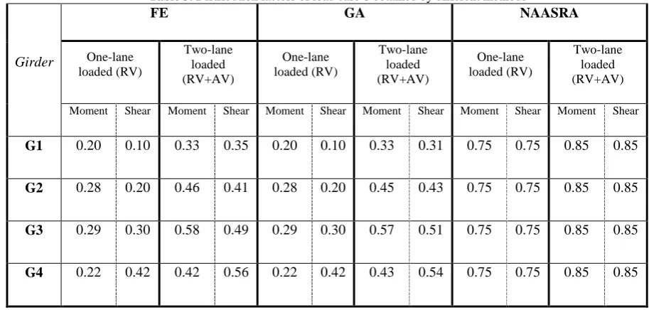
deck with girders to transfer the external loads to adjacent girders as observed in the previous load cases. 5

Table 3. Distribution factors of load case 6 obtained by different methods

6

Girder

FE GA NAASRA

One-lane loaded (RV)

Two-lane loaded (RV+AV)

One-lane loaded (RV)

Two-lane loaded (RV+AV)

One-lane loaded (RV)

Two-lane loaded (RV+AV)

Moment Shear Moment Shear Moment Shear Moment Shear Moment Shear Moment Shear

G1 0.20 0.10 0.33 0.35 0.20 0.10 0.33 0.31 0.75 0.75 0.85 0.85

G2 0.28 0.20 0.46 0.41 0.28 0.20 0.45 0.43 0.75 0.75 0.85 0.85

G3 0.29 0.30 0.58 0.49 0.29 0.30 0.57 0.51 0.75 0.75 0.85 0.85

G4 0.22 0.42 0.42 0.56 0.22 0.42 0.43 0.54 0.75 0.75 0.85 0.85

Note: RV= Reference Vehicle, AV= Accompanying vehicle 7

8

5.

Load assessment ratios

Previous sections have presented the effects of vehicular loadings using a component-level basis for different 10

structural responses. This part addresses the influence of considering a global-level response when evaluating 11

existing bridges. In addition to the rating factor given in AS 5100.7, a jurisdictional approach like the TMR 12

approach has assessment ratios with three Tiered approaches (Tier 0 to Tier 2) for assessment of bridges in state 13

and national highways. The following ratios were devised to illustrate the effect of modelling approaches on load 14

assessment. Developed ratios were adopted based on tiered assessment ratios, so they can be applied to all levels 15

of condition appraisal from basic assessment (Tier 0) to more advanced analysis (Tier 2). 16

load case FE model comparison ratio =

Reference vehicle

load effect

load effect

(1)

load case GA model comparison ratio =

Reference vehicle

load effect

load effect

(2)

1

GA model comparison ratio Modelling comparison ratio =

FE model comparison ratio (3)

2

For modelling comparison ratio, the closer the ratio is to unity, the more consistency and scalability is in the 3

modelling. T44 is considered as a reference vehicle due to the fact that the majority of existing bridge stocks in 4

Australia were designed as 44t semi-trailer [28]. All the moving load cases (load Cases 2 to 8) with similar 5

positioning, speed and accompanying vehicle were repeated for the reference vehicle and the maximum load effect 6

for the desired component was selected. Minimum load effects to be checked for superstructure are external and 7

internal girders (moment, shear, torsion, and combination), deck slab (moment and shear) and cross girders [10]. 8

Thus, relevant load cases chosen for comparison are 2, 3, 7 and 8. 9

Load assessment factors such as dynamic load allowance, accompanying lane factor and live load factor are 10

not included and only un-factored load effects were considered. Detailed full load case analysis with inclusion of 11

road authority load factor requirements can be accomplished using modelling ratios for load envelope due to live 12

loads for capacity checking. Despite the fact that individual components of each model had different values in 13

component-level comparisons, the overall difference is very marginal when the maximum effect is chosen for 14

each load case in a global-level comparison. It is apparent from Figure 10 that even when modelling approaches 15

which have discrepancies at component-level, the difference drops notably when a global-level of load effects are 16

considered. An advantage of proposed modelling ratios is for checking analytical models against a validated 17

model. For instance, if the FE model was validated using field measurements and a corresponding grillage model 18

was required or vice versa, then any point falling in the FE model region (i.e., below compatibility line), would 19

be regarded as a non-conservative result for that particular load case and analytical model. Likewise, any point 20

above the compatibility line needs further refinement to match the validated numerical model. Another use of 21

modelling ratios is for comparison of peak effects (global-based analysis) induced by vehicular loading against 22

design load which could be either designed vehicle class or design standard like AS 5100.5 [20]. Shear capacity 23

has been identified by TMR guidelines as a major strength deficiency in concrete bridges due to poor shear 24

investigation can be done to assess the shear in concrete bridges. For such purposes, girders or other primary load-1

carrying members are separately assessed under vehicular loadings. 2

3

Fig. 10 Comparison of modelling ratios 4

This comparison highlights the fact that level of accuracy in modelling is essential for bridge assessment, 5

particularly when component analysis rather than global analysis is involved. To gain better results for the real 6

response of bridges for assessment; existing conditions, time dependant properties, reinforcement modelling and 7

material nonlinearity (geometric nonlinearity if applicable) need to be included in modelling [29,3]. There are 8

many other parameters that need to be included for assessment which were not considered during the original 9

design. Damage detection and structural system identification using various SHM techniques provide assessment 10

information that can be considered for bridge assessment which result in more reliable estimation, since in-service 11

conditions are reflected in modelling rather design condition documented in the original drawings. Proposed 12

flowchart for validation of numerical modelling is shown in Figure 11. This process is applicable for any type of 13

bridge profiles and load assessment. It can also be extended to a range of vehicles for various load effects of 14

structural components (superstructure and substructure) for serviceability and strength limit states using load 15

factors and other provisions prescribed by state department of transportation. 16

Fig. 11 Flow chart of numerical modelling validation process 17

Flowchart can be used with either modelling technique, or a combination of both. Since most of the existing 18

bridges already have a GA model from their previous assessment, such GA models can be enhanced by addition 19

of SHM data. If the GA model is not capable of doing a detailed assessment, then the corresponding FE model 20

can be generated using modelling ratios. If one modelling approach is chosen, then the modelling ratios can be 21

reconstructed to build the numerical model for families of bridges with similar configurations. Also, the modelling 22

ratios may be used for comparison of updated FE or GA models with those of reference models to establish the 23

state of change for each bridge element due to live load. This enables to track the state of damage in structural 24

elements over time since for each assessment, the numerical model is calibrated, which can be compared against 25

previous analytical models. For the rapid comparison, only specific elements from both models can be compared 26

compatibility. For that purpose, at least some data from existing conditions are needed to validate either numerical 1

model, and then calibrate other computer models. This is a very important consideration because merely using 2

design documents for assessment may not give reliable results. 3

Although the existing assessment approaches in Australia are helpful for quantifying the risks associated with 4

heavy freight vehicles, still the traditional design-based methods are used for structural capacity check and usually 5

the maximum load response is considered for any live load analysis instead of component-based analysis. Current 6

best practice is to use simplified numerical model for bridge load assessment. The nominal capacities of bridge 7

components are determined from the design drawings if there is no severe damage (which is verified by visual 8

inspection or previous records).Then, analytical load effects due to different truck loadings are evaluated and 9

subsequently, the bridge is rated. A drawback of this approach is that truck loading is not always feasible due to 10

fiscal constraints, traffic interruption and possible structural deficiencies of the bridge to handle heavy truck 11

loading. In addition, critical modelling information such as boundary conditions and material properties are taken 12

from design blueprints. By using the proposed flowchart, less conservative assessment could be achieved because 13

a baseline model can be made much easier since the numerical model is calibrated; which is applicable to family 14

of similar bridges that need load assessment or analytical model for field test planning. Also, calibrated model 15

may be used for permit access, change to configurations of as-of-right vehicles, future assessments and will enable 16

asset managers to check the structural integrity of their bridges after extreme events. In an event where an old 17

bridge has no design plan, using on-site geometrical measurement and ambient traffic as source of excitation with 18

no traffic closure; operational modal analysis can be implemented. Such approach considerably reduces the cost 19

of testing and uncertainty since analytical model is coupled with in-service conditions for global and component-20

based analysis. 21

6.

Conclusion

It is well established from the literature that most of bridges analysed by FE method could also be analysed by 23

GA. From the design point of view, both methods can be chosen and it is more related to individual preference. 24

However, bridge assessment requires more detailed information and accurate modelling compared to design. This 25

study was set out to gain a better understanding of GA and FE methods for application of SHM techniques for 26

bridge load assessment. Bridge responses under several vehicular loadings with diverse intensity, speed and 27

direction were investigated. Results of numerical analyses revealed that when component-level analysis is 28

had much lower difference in both models when global-level analysis was undertaken. Based on the results of 1

modelling ratios, it was observed that even large difference in component-level analysis can be masked when 2

global-level analysis are considered. Developed flowchart for validation of numerical model can assist in better 3

estimation of load effects on component-basis. Doing so, cost of modelling can be justified as any unnoticed and 4

unintentional errors can be detected to prevent conservative estimation. Considering the changes of AS 5100.7 5

made to bridge assessment, it is concluded that applicability of SHM techniques for numerical modelling must be 6

incorporated in the bridge assessment with respect to capability of modelling techniques for damage simulation 7

and assessment, sensor placement, field test planning and model updating. When the modelling flowchart is 8

employed in the codified bridge assessment approaches, more accurate estimation of bridge capacity is made since 9

in-service properties obtained by SHM techniques are used; and the updated numerical model can be used for 10

future assessments. 11

7.

Acknowledgment

The first author is thankful for full financial support provided by Queensland University of Technology. Also, 13

valuable comments provided by Prof Eugene O’Brien for grillage modelling is appreciated. 14

8.

References

16

1. Shaw P, Pritchard R, Heywood R (2014) Bridge analysis: are we data managers or engineers? In: Proceedings 17

of 9th Austroads Bridge Conference, Sydney, New South Wales, Australia 18

2. Morrison S, Moses J (2011) Benefits and uses of FE modelling in bridge assessment and design. In: Proceedings 19

of the 8th Austroads Bridge Conference, Sydney, New South Wales, Australia 20

3. Jamali S, Chan THT, Thambiratnam DP, Ross Pritchard, Nguyen A (2016) Pre-test finite element modelling 21

of box girder overpass-application for bridge condition assessment. In: Proceedings of the Australasian Structural 22

Engineering Conference (ASEC), Brisbane, Australia 23

4. Jaeger LG, Bakht B (1982) The grillage analogy in bridge analysis. Can. J. Civ. Eng. 9 (2):224-235 24

5. Lu P, Li F, Shao C (2012) Analysis of a T-Frame Bridge. Mathematical Problems in Engineering 2012. 25

doi:http://dx.doi.org/10.1155/2012/640854 26

6. Sadeghi J, Fathali M (2012) Grillage analogy applications in analysis of bridge decks. Aust. J. Civil Eng. 10 27

(1):23-36. doi:10.7158/c10-670.2012.10.1 28

7. Yang M, Zhong H, Telste M, Gajan S (2016) Bridge damage localization through modified curvature method. 29

J Civil Struct Health Monit 6 (1):175-188. doi:10.1007/s13349-015-0150-7 30

8. McElwain BA, Laman JA (2000) Experimental verification of horizontally curved I-girder bridge behavior. J. 31

9. Krzmarzick DP, Hajjar JF Load rating of curved composite steel I-girder bridges through load testing with 1

heavy trucks. In: Structures Congress, 2006. doi:10.1061/40889(201)149 2

10. Queensland Department of Transport and Main Roads (2013) Tier 1 Heavy Vehicle Bridge Assessment 3

Criteria. TMR 4

11. Australian Standards (2017) Bridge Design- Part 2: Design Loads (AS 5100.2). Sydney, Australia 5

12. Australian Standards (2017) Bridge Design- Part 7: Bridge Assessment (AS 5100.7). Sydney, Australia 6

13. Pritchard R (2014) AS 5100.7 bridge assessment: 2014 revision. In: Proceedings of the 9th Austroads Bridge 7

Conference, Sydney, Australia 8

14. Pritchard R (2017) Revision of Australian Standard AS 5100 part 7: bridge assessment. In: Proceedings of the 9

10th Austroads Bridge Conference, Melbourne 10

15. Hambly EC (1991) Bridge deck behaviour. Second edn. E & FN Spon, London 11

16. Qaqish M, Fadda E, Akawwi E (2008) Design of T-beam bridge by finite element method and AASHTO 12

specification. KMITL Science Journal 8 (1):24-34 13

17. Jenkins D (2004) Bridge Deck Behaviour Revisited. In: Proceedings of the 5th Austroads Bridge Conference, 14

Hobart, Tasmania 15

18. Obrien EJ, Keogh D, O'Connor A (2014) Bridge deck analysis. Second edn. CRC Press, Florida 16

19. Surana C, Agrawal R (1998) Grillage analogy in bridge deck analysis. Narosa, New Delhi 17

20. Australian Standards (2017) Bridge Design - Part 5: Concrete (AS 5100.5). Sydney, Australia 18

21. Reddy JN (2006) Theory and analysis of elastic plates and shells. Second edn. CRC press, Bosa Roca 19

22. Moravej H, Jamali S, Chan THT, Nguyen A (2017) Finite Element Model Updating of civil engineering 20

infrastructures: a review literature. In: International Conference on Structural Health Monitoring of Intelligent 21

Infrastructure, Brisbane, Australia 22

23. Hambly E, Pennells E (1975) Grillage analysis applied to cellular bridge decks. Structural Engineer 53 (7) 23

24. National Association of Australian State Road Authorities (1976) NAASRA Bridge design specification. 24

Sydney, Australia 25

25. AECOM Australia (2002) Investigating the Development of a Bridge Assessment Tool for Determining 26

Access for High Productivity Freight Vehicles (AP-R398-12). 27

https://www.onlinepublications.austroads.com.au/items/AP-R398-12. Accessed 1 June 2016 28

26. Lake N, Ngo H, Kotze R (2014) Review of AS 5100.7 Rating of Existing Bridges and the Bridge Assessment 29

Group Guidelines (AP-R452-14). https://www.onlinepublications.austroads.com.au/items/AP-R466-14. 30

Accessed 1 June 2016 31

27. Lake N, Seskis J, Ngo H, Kotze R (2014) Review of axle spacing mass schedules and future framework for 32

assessment of heavy vehicle access applications (AP-R466-14). 33

https://www.onlinepublications.austroads.com.au/items/AP-R466-14. Accessed 1 June 2016 34

28. Pritchard R, Heywood R, Shaw P (2014) Structural assessment of freight bridges in Queensland. In: 35

Proceedings of the 9th Austroads Bridge Conference, Sydney, New South Wales, Australia 36

29. Schlune H, Plos M (2008) Bridge Assessment and Maintenance based on Finite Element Structural Models 37

1

2

3

4