MATHEMATICAL REFLECTION APPROACH TO INSTRUMENTAL VARIABLE ESTIMATION METHOD
FOR SIMPLE REGRESSION MODEL
Anwar Saqr1 and Shahjahan Khan2 1Al Buraimi University College, Oman
2School of Agricultural, Computional and Environmental Sciences University of Southern Queensland, Toowoomba, Australia
Emails: [email protected] - [email protected]
ABSTRACT
The measurement errors problem is endemic in many econometric studies, and one of the oldest known statistical problems. Instrumental variable (IV) method is one of the popular solutions adopted to deal with the mismeasured variables in statistical and econometric analyses. This paper proposes an efficient IV estimator to the parameters of the simple regression model where both variables are subject to measurement errors. The proposed IV is defined using simple mathematical transformation of the manifest independent variable (mismeasured variable). The proposed method is straightforward, and easy to implement. The theoretical superiority of the proposed estimator over the existing IV based estimators due to Wald (1940), Bartlett (1949), and Durbin (1954) is established by analytical comparison and geometric expositions. Simulation based numerical comparisons of the proposed estimator with four different existing estimators are also included.
Keywords: Simple regression model, Error-in-Variables model, Instrumental variable.
1- INTRODUCTION
The measurement errors problem is a very old problem, and it has
been considered by a host of authors since the late nineteenth century.
This problem is seldom taken into fully account, although it has very
serious consequences on the statistical inference.
In reality the measurement errors in data are inevitable and exist in
almost all the applied fields. Linnet (1993) states, “It is rare that one
of the measurement methods is without error.” The motivation of
proposed methods in the literature of measurement error is to
eliminate, or at least reduce implications of the measurement error on
the estimator of parameters. The measurement error problem it is
often given prominence in econometrics texts, for example Judge et
al (1980), Stock et al (2003), Hill et al (2008), Wooldridge (2010),
but it is rarely included in statistical texts (Gillard, 2005). This
problem has been studied in depth by some authors such as Fuller
(2006), Cheng and van Ness (1999), Casella and Berger (1990),
Sprent (1969), Dunn (2004), and Kendall and Stuart (1973, chap. 29).
They concentrated on the maximum likelihood principle and
summarize correction formulae for measurement error models based
on assumptions of additional information.
However despite all these efforts the challenge is still looming, since
Riggs et al. (1978) stated that no one method of estimating the true
slope is the best method under all circumstances. Cheng and van Ness
(1999) stated that some users object to the use of these side conditions
and prefer other methods of approaching the measurement error
The alternative method which was pioneered to overcome the
measurement error problem since 1920 is the instrumental variables
approach (see Goldberger (1972) for a historical review). This
approach provides supplementary information to make the
parameters identifiable (cf Cheng and van Ness, 1999, p.93). This
method is one of the popular solutions adopted to deal with the
mismeasured variables in statistical and econometric analyses by
Wald (1940), Durbin (1954), and Sargan (1958). Most recently, Chen
et al. (2014) reviewed and investigated the existing
errors-in-variables estimation methods and their applications in finance
research. Almeida et al. (2010) have argued and presented an
alternative instrumental method to deal with measurement error
problems.
Instrumental variable (IV) technique requires defining an IV that is
uncorrelated with the model error but highly correlated with the
independent variable. Wald (1940) suggested to use -1 and +1 for
values less than or greater than the median of the manifest variable,
Bartlett proposed to divide the values in three equal groups and use
the first and third groups, and Durbin used the ranks of the values to
define the IV. In each of the method there is loss of information (for
not using actual values and dropping some of the data points), and
there are different formulae to find the sum of squares error, and
hence lead to different mean sum of square error, making the analysis
incomparable.
The IV method has been used for studying the natural and
quasi-natural experiments such as Miguel et al. (2004) studied the weather
shocks to identify the effect of changes in economic growth on civil
variables have been widely used to reduce bias from omitted
variables in estimates of causal relationships in randomized
experiments such as the effect of schooling on earnings. They have
presented a survey of the history and uses of instrumental variable
technique. Cheng and van Ness (1999) stated that the instrumental
variable method suits all kinds of regression with random regressors
for which the explanatory variables are correlated with the errors.
Bowden and Turkington (1981), and Martens (2006) introduced the
details of general treatment of instrumental variables and their
applications and limitations.
It is worth noting that the greatest drawback of IV approach is how
or where to find valid instrumental variable, which it is not easy to
obtain. Therefore, this paper proposes an instrumental variable which
is easier to obtain in practice to estimate the parameters of bivariate
errors-in-variables model. The proposed instrumental variable is
defined using reflection of the observed values of the independent
variable. The proposed modified method uses the reflection of the
manifest values of the independent variable to define IV estimator.
The using of the reflections of the observed values of the independent
variable in defining the IV method provides a much better estimator
of the slope and intercept parameters. It also reduces the mean sum
of squares error. The analysis of variance and regression inferences
based on the reflections have much better statistical properties than
any other form of the IV estimator (Saqr and Khan, 2012).
In the next section the measurement error regression model is
introduced. Section 3 covers the existing estimation methods for the
measurement error model. The proposed modified estimator based
is provided in Section 4. The superior properties of the modified
estimator are discussed in Section 5. A simulation study is presented
which compares the proposed estimator with five different existing
estimators are provided in Section 6, and some concluding remarks
are given in Section 7.
2- MEASUREMENT ERROR MODELS
In the conventional notation, let
j denote the true measurement onthe independent variable. This is also called the latent independent
variable. In the presence of measurement error the actual
observations are different fromj. Let
x
be the observable, ormanifest variable of the independent variable. When the true value of
the latent variable
j is observed, the commonly used classicalsimple linear regression model is represented by
0 1
,
1, 2,
, ,
j j
e
jj
n
(1)where j is the jth realisation of the latent dependent variable, j
is the fixed jth value of the independent variable, and
e
j is theequation error for j 1, 2,,n. It is assumed that the equation error
j
e is independently distributed with constant but unknown variance,
that is, 2
~ (0, )
j e
e N .
If there is error in the independent variable, the actual observed value,
j
x , is not the `true' value of the independent variable. The observed
value of the independent variable contains measurement error given
,
1,2,
, ,
j j jx
j
n
(2)where j is the measurement error, and is assumed to be distributed
as 2
(0, )
N . Note that, unlike
j,x
j is a random variable which isassumed to be distributed as 2
( x, x).
N The model with the fixed
jis called the functional model, and the model with the random or
stochastic
x
is called the structural model.The simple regression model with measurement error in the
independent variable can be expressed as
0 1
,
1, 2,
, ,
j
x
jv
jj
n
(3)where vj ej
1 j. Note in equation (1)
j ande
j areindependent, but in equation (3),
x
j andv
j are not independent. Sothe application of least squares method is not valid for the models
with measurement error. Thus, unlike for the model in (1), the
validity of the estimator of the slope and intercept of the model in (3)
is not obvious. However, Fuller (2006, p. 3) assumes that
j,
j andj
e
are mutually independent for the estimation of the parameters. Italso assumes that the reliability ratio, kx
x2 2
is known, where
2
x
is the variance of the manifest variablex
j, and 2 is the varianceof the latent variable
j.The ordinary least squares (OLS) estimator of the regression
parameters for the functional model are
1 2 0 1
ˆ
S
, and
ˆ
ˆ
,
S
(4)where 2 2 1 1 1 1 ( )( ), ( ) , 1 1 n n
j j j
j j S S n n
(5)in which 1 1 n j j n
and1 1 n j j n
. The estimators of slope andintercept parameters are well known to be the best linear unbiased
estimators if there is no measurement error in the variables.
The sampling distribution of the estimator of the regression
parameters is given by
2 2 2
0 0 2
2 1 1 2 2 1 ˆ ~ , . ˆ 1 e
n S S
N S S (6)
The unbiased estimator of the error variance
e2 is given by1 2
ˆ
e(
n
2)
SSE
eS
e,
where 2
1
ˆ
(
) ,
n
e j j
j
SSE
in which
ˆ
j
ˆ
0
ˆ
1 j is the estimated value of
j. Also,2
e
SSE
e
follows a
2 distribution with (n 2) degrees offreedom.
In the presence of measurement error, the
x
values are observedinstead of
j,
then the least squares method yields the estimator ofthe slope as
1 2 0 1
ˆ
x, and
ˆ
ˆ
.
x x x
x
S
x
S
(7)It can be easily shown that ˆ1x is a biased estimator of 1. Also, the
above estimator is not a consistent estimator of 1.
Note that the regression parameters are different for the model with
the manifest variable than the model with the latent variable. Even
though the aim is to estimate and test
0 and
1, in reality onemay end up estimating and testing 0x and
1x if one fully reliesupon
x
, and over looks the presence of the measurement error.4- INSTRUMENTAL VARIABLE (IV) ESTIMATOR
In the presence of measurement error in the independent variable
the IV estimator for the regression parameters is defined as
1
ˆ
(
z x
)
z
,
where
β
ˆ
(
ˆ
0,
ˆ
1)
is the vector of estimator of the intercept andslope parameters of the model
where
1 2
1 1 1
n x
x x x
and 1 2
1
1
1
,
n
z
z
z
z
in which
z
j's are the values of the second row of the instrumentalvariable
z
. The selection of the values ofz
j's require that it is highlycorrelated with the independent variable but uncorrelated with the
model errors. The variance-covariance of the above estimator vector
is given by
2 -1 -1
ˆ
var( )=
β
(z x) (z z)(z x) .
(9)Obviously the value of the estimator and the variance depend on the
choice of
z
(see Johnson, 1972). For instance, the Wald method, assuggested by Maddala (1988), defines
z
by assigningz
j to be -1 or+1 depending upon if
x
j is smaller or larger than the median valueof the manifest variable. The estimator of slope under this choice of
IV is
2 1
1
2 1
ˆ
,
W
x
x
where
1 is the mean of
-values associated with the values ofx
median value of
. Bartlett (1949) followed the same selectioncriterion of
z
j's but suggested the exclusion of the middle 1/ 3 of thevalues, and his estimator is based on the lower and upper 1 / 3 of the
values of
x
and the associated
s . The estimator is expressed as3 1
1
3 1
ˆ
,
B
x
x
where
1 is the mean of
-values associated with the smallest 1/ 3of the values of
x
, and
3 is that for the largest 1 / 3. Durbin (1954)proposed to use the rank of
x
asz
j's. His method yields thefollowing estimator of the slope parameter
1
1 1
ˆ
n/
n,
D j j
j j
j
j x
but does not define the estimator of the intercept.
The IV method of estimation of the regression parameters does not
require any strict assumptions such as the ratio of error variances is
known. But the actual estimator depends on how the IV is defined, as
the definition of
z
affects both the estimator and its variance. Ingeneral, the available methods of defining IV causes a significant loss
of sample information (data) either by replacing the observed values
of the independent variable by -1 or +1, or exclusion of some data, or
due to ranking of data.
The idea of the proposed estimator of slope is based on using the
reflection variable of the manifest independent variable as IV
variable. The proposed IV variable is obtained by reflecting all values
of the manifest independent variable about the unfitted regression
line. This is essentially done by a transformation of the observed
values of the independent variable to their reflection on the Euclidean
plane. In the conventional notation, the reflection of the manifest
independent variable
x
j
j j (with measurement error
j) for1, 2, , ,
j n can be defined as
*
0
ˆ
cos 2
(
x) sin 2 ,
x
x
(10)where ˆ0xis the least squares estimate of the intercept parameter,
is the angle measure defined as arctanˆ1x in which ˆ1x is the
least squares estimate of the slope parameter in the manifest model,
and Cos, Sin are the usual trigonometric cosine and sine functions
respectively. For the definition of reflection points on the Cartesian
plane readers may see (Vaisman 1997, p. 164-169; Saqr and Khan,
2012).
The proposed reflection method requires to compute the reflection of
all data points, and the use of the transformed values of
x
, i.e.x
*, in defining the IV to fit the regression line of . The IV estimator ofthe slope parameter under the proposed modified method is
* 1
1 2
ˆ
(
)
, and
ˆ
x,
r r R
x
S
z x
z
S
* *
2 * *
* * *
1 1 2
1 1 1
, , ( )( ).
n
r x x x x x j j
j n
Z S S and S x x x x
x x x
The proposed estimator of the slope parameter of the simple
regression model using IV based on the reflection of
x
is*
1 2
ˆ
x.
R x
S
S
(11)From (11), it is easy to show that
S
xy
S
y andS
x2
S
2
S
2.It can be found that
* xy x
sin 2 ,
x y
S
S
SSE
(12)where
is as defined in equation (10), andSSE
x is the sum of squares error for the manifest model. The above result follows from the fact that*
0
ˆ
cos 2
(
) sin 2
j j j j x j
x
x
x
x
0
ˆ
(cos 2
1)
sin 2
sin 2
j j x
x
2 2
(2sin
)
sin 2
sin 2
2sin
j j
x
x
2
(
j) sin 2
(
x
jx
)2sin
,
(13)where
x
*j is the reflection ofx
j. Multiplying both sides of the aboveequation by
j and taking sum overj, yields* 2
(xjxj)j ( j ) jsin 2 (xjx)j2sin
*
2 2
sin 2
2 sin
x x
x
S
S
S
S
*
,
sin 2
x x x xS
S
SST
SSR
SSE
(14)where 2
S SST is the sum of squares total, SSRx is the sum of
squares regression, and SSEx is the sum of squares error for the
regression of
onx
. Note that 21
2sin ˆ
tan
sin 2 x
.
Then using equation (10), it can be written as
*
1 2 2 2 2
sin 2
ˆ
x x xx
S
SSE
S
S
S
S
S
S
*1 2 2 2 2 2
sin 2
sin 2
ˆ
x x x x.
R x
S
S
SSE
S
SSE
S
S
S
S
S
Let
* be the ratio of the vertical error variance
v2 and horizontalerror variance
2, that is * 2 2 v .Based on the assumption * *
sin 2 x x S S
, then
* *
1 2 2 2
ˆ
x xR
x x
S
S
S
S
S
S
* * 2
(
x)
x(
)
x x
S
S
S
S
S
S
which leads to * 2
,
x x
S
S
S S
and finally simplificationyields
*
1 1
2 2
, hence
ˆ
ˆ
.
x
R x
S
S
S
S
(16)6- GEOMETRIC EXPLANATION OF THE PROPOSED ESTIMATOR
The presence of measurement error in the independent variable and
its impact on the estimator of the slope as well as how the proposed
method ‘treats’ the measurement error can be explained by graphs.
The graphical representation also explains how the actual estimator
of the slope is recovered by the new method. Figure 1 represents the
sum of squares and sum of products associated with the definition of
the estimators of slope both for the latent and manifest variables. This
graph represents the presence of measurement error in the
independent variable as well as the two estimators of the slope
parameter. On the other hand Figure 2 displays the same along with
that of the reflection of the manifest variable and three estimators of
Figure 1: Graph representing the sum of squares and products in the presence of measurement error in the independent variable.
From Figure 1, the true estimator of the slope when the latent variable
is available, that is, ˆ1
is represented by the tan of BAC of
ABC. In the absence of the values of the latent variable this is
unavailable. But for the manifest variable one can find the estimator
of the slope to be ˆ1x which is represented by the tan of DAE
of ADE. Note that here DC (or equivalently BE) represents the sum
of squares of measurement error
(
S
2).
Furthermore, under theassumptions of E[
]0 and E[]0, we have BC DE orx
S S . Finally, ˆ1 2 ,
S BC
S A C
and ˆ1 2 .
xy x
x
S ED
S A D
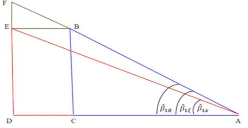
Figure 2: Graph representing the sum of squares and products when the measurement error in the independent variable is 'treated' by reflection.
The introduction of the reflection of the manifest variable changes
ADE of Figure 1 to ADF in Figure 2. In fact the main difference
between the two Figures is that Figure 2 has the small BEF added
to Figure 1. This triangle represents the effect of the reflection of the
manifest variable. From Figure 2 the estimates of the slope are
1 2
ˆ
xx x
S
DE
S
DA
(17)1 2
ˆ
S
BC
S
A C
(18)*
1 2
ˆ
x.
R x
S
FD
S
A D
(19)Since the tan of BAC represents the estimator ˆ1
and tan of
DA F
7- SIMULATION STUDY
In this section, simulated data are used when both the dependent and
independent variables are subject to measurement error. This study
reveals that the performance of proposed estimator (RIV) is better
than OLS estimator and other estimators proposed by Wald (1940)
(Two g ), Bartlett (1949)(Thrg), and Durbin (1954) (Dur).
Here calculations are based on the generated values of variables for
preselected values of 0 0,
1
1
, latent variable
~N(0,36),2 16
, and
e29. The simulation is based on 10,000 replications [image:17.595.174.441.278.435.2]using MATLAB software.
Figure 3: Graphs of the estimated slope (a) and the mean absolute error (b) for five different estimators, proposed instrumental variable estimator (R IV), Wald's estimator (T w og), three-group estimator (Thrg), Durbin estimator (Dur), and ordinary least squares estimator (OLS).
To show the behavior of the above estimators we selected samples
estimators from the simulated data and find their means and mean
absolute errors (MAE) for each of the five estimators.
Figures 3a and 3b show the estimated slope and the mean absolute
error for five different estimators. From the above graph it is evident
that the proposed instrumental variable estimator (RIV) is
consistently better than the other four estimators. Clearly the RIV
estimator is much closer to the true value of
1 than other fourestimators. In fact, the proposed RIV estimator is consistently closest
to the true value of the slope for all sample sizes.
8- CONCLUDING REMARKS
This paper considers the simple regression model with measurement
error in both dependent and independent variables. It also proposes a
new estimation procedure based on the idea of a new instrumental
variable which is defined from reflection of the manifest variable. It
compares the existing methods with proposed new method. Unlike,
some of the existing methods it does not lose information.
The simulation study demonstrates the fact that the proposed method
significantly reduces the mean absolute error than the currently used
IV methods. As such, the coefficient of determination of the proposed
method is higher than that of the existing IV methods. Surprisingly,
the proposed IV method recovers the true estimator of the slope,
1
ˆ ,
from the manifest variable and stochastic model even if the truevalues of the latent independent variable are unobservable. The same
ACKNOWLEDGEMENTS
The authors appreciate the valuable comments and suggestions from
two unknown referees, and the Editor that improved the content of
the paper.
REFERENCES
1. Almeida, H., Campello, M., and Galvao, A.F. (2010).
Measurement errors in investment equations. Review of
Financial Studies, 23(9), 3279-3328.
2. Angrist, J., and Krueger, A.B. (2001). Instrumental
variables and the search for identification: From supply and demand to natural experiments (No. w8456). National Bureau of Economic Research.
3. Bartlett, M.S. (1949). Fitting a straight line when both
variables are subject to error. Biometrics, 5(3), 207.
4. Bowden, R.J., and Turkington, D.A. (1981). A
comparative study of instrumental variables estimators
for nonlinear simultaneous models. Journal of the
American StatisticalAssociation, 76(376), 988-995.
5. Casella, G. and Berger, R.L. (1990). Statistical Inference.
Wadsworth and Brooks/Cole, Pacific Grove, CA.
6. Chen, H.Y., Lee, A.C., and Lee, C. F. (2014). Alternative
errors-in-variables models and their applications in
finance research. The Quarterly Review of Economics
and Finance.
7. Cheng, C.L. and Van Ness, J.W. (1999). Statistical
regression with measurement Error. Arnold, London.
8. Dunn, G. (2004). Statistical Evaluation of Measurement
Errors. (2nd Edition). Arnold, London.
9. Durbin, J. (1954). Errors in variables. Revue de l'Institut
10. Fuller, W. A. (2006). Measurement Error Models. Wiley Series in Probability and Statistics.
11. Gillard J., T. (2005). Method of moments estimation in
linear regression with errors in both variables. Cardiff University School of Mathematics Technical Report, Cardiff, Wales, UK.
12. Goldberger, A. S. (1972). Structural equation methods in
the social sciences. Econometrica: Journal of the
Econometric Society, 979-1001.
13. Hill, R.C., Griffiths, W.E., and Lim, G.C. (2008).
Principles of Econometrics. (Vol. 5).
14. Hoboken, NJ: Wiley. Johnson, J. (1972). Econometric
Methods. McGraw Hill Book Company: New York.
15. Judge, G.G., Griffiths, W.E., Carter, R. and Lee, T.C.
(1980). The Theory and Practice of Econometrics. Wiley,
New York.
16. Kendall, M.G. and Stuart, A. (1973). The Advanced
Theory of Statistics. (Vol.2). Griffin, London.
17. Linnet, K. (1993). Evaluation of regression procedures
for methods comparison studies. Clinical Chemistry 39,
424-432.
18. Maddala, S., (1988). Introduction to Econometrics. (2nd
edition). International Inc. Prentice Hall.
19. Martens, E.P., Pestman, W. R., de Boer, A., Belitser,
S.V., and Klungel, O.H. (2006). Instrumental variables:
application and limitations. Epidemiology, 17(3),
260-267.
20. Miguel, E., Satyanath, S., and Sergenti, E. (2004).
Economic shocks and civil conflict: an instrumental
variables approach. J Polit Econ, 112(4), 725-753.
21. Saqr, A., Khan, S. (2012). Reflection method of
estimation for measurement error models. Journal of
Applied Probability and Statistics, 7(2), 71-88.
22. Sargan, J.D. (1958). The estimation of economic
relationships using instrumental variables. Econometrica,
26(3), 393.
23. Sprent, P. (1969). Models in Regression and Related
24. Stock, J.H., and Watson, M.W. (2003). Introduction to
Econometrics. (Vol. 104). Boston: Addison Wesley.
25. Vaisman, I. (1997). Analytical Geometry. Series on
University Mathematics.
26. Wald, A. (1940). The fitting of straight lines if both
variables are subject to error. The Annals of Mathematical
Statistics, 11(3), 284-300.
27. Wooldridge, J.M. (2010). Econometric Analysis of Cross