ORIGINAL ARTICLE
Estimation of metabolite networks with regard to a specific
covariable: applications to plant and human data
Georgios Bartzis1 · Joris Deelen2 · Julio Maia3 · Wilco Ligterink4 ·
Henk W. M. Hilhorst4 · Jeanine‑J. Houwing‑Duistermaat1,5 · Fred van Eeuwijk6 · Hae‑Won Uh1
Received: 19 April 2017 / Accepted: 30 August 2017 / Published online: 22 September 2017 © The Author(s) 2017. This article is an open access publication
Methods Alternative to using the original metabolite val-ues, the total information is decomposed by utilizing a linear regression model and the part relevant to 𝐗m is further used.
For two datasets, two different network estimation methods are considered. The first is weighted gene co-expression net-work analysis based on correlation coefficients. The second method is graphical LASSO based on partial correlations.
Results We observed that when using the parts related to the specific covariable of interest, resulting estimated net-works display higher interconnectedness. Additionally, sev-eral groups of biologically associated metabolites (very large density lipoproteins, lipoproteins, etc.) were identified in the human data example.
Conclusions This work demonstrates how information on the study design can be incorporated to estimate metabolite networks. As a result, sets of interconnected metabolites can be clustered together with respect to their relation to a covariable of interest.
Keywords Network reconstruction · Incorporating relevant information · Metabolites · Study design
1 Introduction
In recent years, network analysis of biological datasets has become an increasingly popular tool for studying the rela-tionships between large numbers of variables that occur in omics research on transcripts, metabolites, proteins and others. In networks, variables are represented by nodes and their relationships, direct and indirect interactions (physi-cal or functional), are represented by edges or links. One is often interested in the joint distribution of a set of variables conditional on a particular covariable. For example, one may want to study the relations between a set of metabolites
Abstract
Introduction In systems biology, where a main goal is acquiring knowledge of biological systems, one of the chal-lenges is inferring biochemical interactions from different molecular entities such as metabolites. In this area, the metabolome possesses a unique place for reflecting “true exposure” by being sensitive to variation coming from genetics, time, and environmental stimuli. While influenced by many different reactions, often the research interest needs to be focused on variation coming from a certain source, i.e. a certain covariable 𝐗m.
Objective Here, we use network analysis methods to recover a set of metabolite relationships, by finding metabo-lites sharing a similar relation to 𝐗m. Metabolite values are
based on information coming from individuals’ 𝐗m status
which might interact with other covariables.
* Georgios Bartzis [email protected]
1 Department of Medical Statistics and Bioinformatics,
Leiden University Medical Center, Einthovenweg 20, 2300 RC Leiden, The Netherlands
2 Department of Biological Mechanisms of Ageing,
Max Planck Institute for Biology of Aging,
Joseph-Stelzmann-Strasse 9b, 50931 Cologne, Germany
3 São Paulo State University, FCA/UNESP, Botucatu,
SP CEP 18610-307, Brazil
4 Wageningen Seed Lab, Laboratory of Plant Physiology,
Wageningen University, Droevendaalsesteeg 1, 6708 PB Wageningen, The Netherlands
5 Department of Statistics, School of Mathematics, University
of Leeds, Leeds LS2 9JT, UK
6 Biometris, Wageningen University, P.O. Box 16,
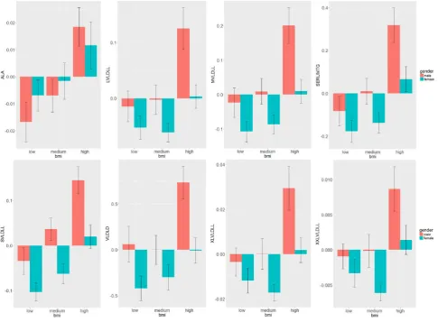
with regard to body mass index (BMI). As an illustration, in Fig. 1 we show the concentrations of eight very large density lipoprotein (VLDL) particles that are associated with BMI and gender in a similar way, i.e. males have higher VLDL concentrations than women; low VLDL concentrations are associated to low and medium BMI categories, and high VLDL concentrations to high BMI. The aim of the current paper is to detect these groups of metabolites with similar relationships by using network analysis.
For network estimation, networks with different features are typically used for representing networks, i.e. undirected or directed networks. In undirected networks, edges connect-ing two nodes do not have a direction indicatconnect-ing a symmetric relationship between them. In biology, undirected network estimation methods based on correlation are often preferred. These methods perform well with large numbers of sam-ples and variables. However, little is known about their per-formance in a small sample setting. Therefore, estimating, describing, visualizing and comparing networks for rela-tively small samples is an ongoing topic of research (Kol-aczyk and Krivitsky 2015). We will consider two methods
of estimating undirected networks. The first is weighted gene co-expression network analysis (WGCNA) based on correlation (Zhang and Horvath 2005; Langfelder and Hor-vath 2008; Zhao et al. 2010). While WGCNA was mainly developed for analysis of gene-expression data, applications on metabolite data have been reported as well (DiLeo et al. 2011; Zhang et al. 2013). WGCNA is based on the concept of scale free networks implying the existence of a few highly connected nodes (hubs) participating in a very large num-ber of metabolic reactions (Zhao et al. 2010). In WGCNA, the strength of the connection between nodes is typically dictated by a similarity measure (Zhao et al. 2010). The sec-ond method is the graphical LASSO (GL) (Friedman et al. 2001, 2008) based on partial correlations. For this Gaussian graphical model (GGM) based method, for two nodes not sharing a direct edge in a network the implication is that they are conditionally independent given all other variables. To obtain a sparse network an L1 penalty can be used. The pen-alty can be determined using a stability selection algorithm (StARS) (Liu et al. 2010) to select a stable set of edges.
[image:2.595.57.543.338.695.2]For describing and comparing the estimated networks using the two methods above, we first characterize the topology of the networks by measuring three types of network concepts Dong and Horvath (2007), Horvath and Dong (2008), i.e. den-sity, centralization, and heterogeneity.
We will consider two different data applications for estimat-ing metabolite networks. In the first application, the metabo-lites are coming from an experiment with seeds in which the desiccation tolerance of these seeds was investigated as a func-tion of genotype and a managed environment condifunc-tion, or treatment. Seeds from two genotypes of the well-known plant
Arabidopsis thaliana, the genotype Columbia-0 (Col-0) and the abscisic acid deficient mutant 2–1 (aba2–1) were selected. Germinated seeds at radicle protrusion were selected and either frozen in liquid nitrogen and stored at −80 °C directly or after 3d of incubation in −2.5 MPa polyethylene glycol (PEG), 5 μM ABA (ABA) or a combination of −2.5 MPa PEG + 1 μM ABA (PEG + ABA). Therefore, four treatments for metabolic profiling have been considered here: (i) no treatment (control), (ii) PEG, (iii) ABA or (iv) both PEG and ABA. In this paper, we focus on estimating metabolite networks based on genotype-related information.
The second application concerns serum metabolites of unrelated individuals coming from the capital region of Fin-land. In this observational study our specific interest lies in estimating networks of metabolites, conditioned on the indi-viduals’ BMI status which might interact with indiindi-viduals’ sex and age.
The rest of the paper is organized as follows. In Sect. 2, we propose our method for selecting information relevant to a certain covariable prior to network estimation. Addition-ally we review some existing network estimation methods. In Sect. 3, we demonstrate our network estimation approaches on metabolite data coming from plants and humans, and we conclude with a Discussion in Sect. 4.
2 Methods
A network consists of a set of nodes (or vertices) connected by a set of edges (or links). In this paper we consider undirected networks of metabolites, where the nodes correspond to the metabolites, and the edges between metabolites represent their relationship. For a network of P nodes, the network structure can be represented by the P×P adjacency matrix 𝐀. For undi-rected networks, the elements aij of the adjacency matrix are
defined as follows:
Note that the adjacency matrix 𝐀 is symmetric and has zeros on the diagonal. The degree or connectivity ki of a
node i is defined as ki= ∑
j≠iaij: i.e. ki equals the number
aij=
{
1, if there is an edge between nodejand nodei
0, otherwise.
of neighbors of node i in the network. In addition to the adjacency matrix we typically consider a P×P intensity
matrix 𝐖 where the elements wij represent the strength of
the relationship between node i and j. If nodes i and j are not linked, the weight wij is equal to zero. Popular choices for
the weights wij are Pearson’s correlation coefficient, mutual information, Euclidean distance, partial correlation and topological overlap.
We will consider absolute Pearson’s correlation coeffi-cient and partial correlations with no self-edges (wii=0).
Analogously to the degree of a node i(ki), the strength or
weighted degree is defined as si=∑j≠iwij. The strength of a node takes into account both the connectivity as well as the weights of the edges.
2.1 Identifying the specific parts of metabolic concentrations relevant to a covariable
The weights represent the relationships between the metabo-lite concentrations. In addition one might be interested in the relationships between specific parts of the metabolite concentrations: for example the part which is related to a covariable of interest. The idea is that metabolites with similar relationships with this covariable will tend to be close to each other in the network (see for example Fig. 1). The parts of the metabolite concentration concerning this specific covariable can be obtained by fitting linear regres-sion models (or ANOVA) to the metabolic variables. Let 𝐘=(𝐘(1),…,𝐘(P)) be the concentrations of P metabo-lites and let 𝐘(p) be the vector of concentrations for the pth metabolite. Assume that 𝐘 follows a multivariate Gaussian distribution 𝐘∼NP(𝝁,𝚺). From m covariables let 𝐗m be the categorical covariable of main interest. The remaining m−1 covariables are denoted as 𝐗(−m) ={𝐗1,𝐗2,…,𝐗m−1
} . Now we propose the following regression model:
where 𝜀p ∼N(0,𝜎2 (p)
)
represents the random noise, 𝜟 is the
space with elements all vectors of length m−1 with all
com-binations of zeros and ones, except all zeros, i.e. 𝜟= {(1, 0,…, 0),(0, 1,…, 0),…,(1, 1,…, 1)}, and ◦ is the
Hadamard product. The term ∑𝜹∈𝜟𝜸𝜹 ∏m−1
j=1 𝐗 𝜹j
j models all
main effects and second and higher order interaction terms of covariables in 𝐗(−m). For example, for m−1=2,
∑
𝜹∈𝜟𝜸𝜹
∏2 j=1𝐗
𝜹j
j =𝜸10𝐗1+𝜸01𝐗2+𝜸11𝐗1◦𝐗2. Similarly,
the term ∑𝜹∈𝜟𝜼𝜹𝐗m◦
∏m−1
j=1 𝐗 𝜹j
j models all terms interacting with 𝐗m. To ensure identifiability of all parameters a level
of the covariable is used as reference category.
(1)
𝐘(p)=𝛽(p)
0 +𝜷
(p)
1 𝐗m+
∑
𝜹∈𝜟
𝜸(𝜹p) m−1
∏
j=1 𝐗𝜹j
j +
∑
𝜹∈𝜟
𝜼(𝜹p)𝐗m◦
m−1
∏
j=1 𝐗𝜹j
j +𝜺
The relevant information for the pth metabolite with regard to the categorical covariable 𝐗m is given by:
Now the edge between node p and q in a network can be based on correlation between 𝐘̂(p) and 𝐘̂(q).
2.2 Network estimation methods
We consider two network approaches, namely WGCNA based on pairwise correlations between metabolites and GL based on partial correlations.
2.2.1 Weighted gene co‑expression network analysis (WGCNA)
WGCNA (Horvath and Dong 2008; Zhang and Horvath 2005; Langfelder and Horvath 2008) has been developed to efficiently analyze the correlation patterns among genes using gene expression data from microarray experiments. Network construction with WGCNA is typically followed by identifying clusters (modules) of highly correlated genes.
Estimation of networks—modeling the intensity matrix
Complex networks may display non-trivial topological fea-tures, such as a heavy tail in the empirical distribution of the degree of the nodes (the number of edges connected to a node). In biology, often networks with many low degree nodes and a few high degree nodes are of interest. Such networks are called scale free. To determine whether a network is scale free the log of the degree frequency (log(P(k))) is plotted against the
logarithm of the degree (log(k)). A linear relationship indicates that the network is scale-free. A scale-free degree distribution can be expressed as P(k) ∝k𝛾 and in a weighted case, i.e. in
the context of WGCNA, the intensity wij can be written on a
logarithmic scale, logwij=𝛾log|| |cor
(
yi,yj)||
| for 𝛾 >1. The
threshold parameter 𝛾 might be chosen in a way such that the
network approximately satisfies the scale-free topology criterion.
In our experience, however, not all biological datasets yield scale free networks. If the network is not scale free 𝛾 will be
determined by the amount of noise in the dataset. For two Gaussian random variables, the magnitude of random noise for correlation coefficients from N samples is 1∕√N. In order to
sufficiently suppress low correlations due to noise, we take the smallest value for 𝛾 in such a way that the total noise is smaller than one (personal communication with Peter Langfelder):
(2)
̂
𝐘(p)=𝜷̂(p)
1 𝐗m+
∑
𝜹∈𝜟
̂
𝜼(𝜹p)𝐗m◦
m−1
∏
j=1 𝐗𝜹j
j .
(3)
P(P−1)
2(√N)𝛾 <1.
Module identification A network might consist of a set of modules of closely interconnected metabolites. Average linkage hierarchical clustering based on a dissimilarity measure is a popular method to define a dendrogram of the network. The modules are obtained by cutting this tree (the two-step dynamic hybrid algorithm) (Langfelder et al. 2008). Here, we will use the following dissimilarity measure:
2.2.2 Graphical LASSO (GL)
GL is another popular approach to obtain a network for a set of variables. Assume that the metabolite concentra-tions (N by P data matrix 𝐘) follow a multivariate Gaussian
distribution with mean vector 𝝁 and variance-covariance
matrix 𝚺. For simplicity we can assume that the data are
centered, i.e. 𝝁=𝟎. The inverse covariance matrix 𝚺−1 is the
precision matrix. When its elements are equal to zero, the pair of metabolites is conditionally independent given the other metabolites. A Gaussian graphical model (Lauritzen 1996) is a network based on these conditional independence relationships.
To estimate 𝚺−1 a penalized log-likelihood approach can be used. Define the precision matrix 𝚯=𝚺−1. Under the
Gaussian model, the log-likelihood function is given by (up to a constant):
where 𝐒=𝐘⊤𝐘∕N is the sample covariance matrix.
Maxi-mizing expression 5 with respect to 𝚯 leads to the maximum
likelihood estimate 𝚯̂. Note that the elements of 𝚯̂ are in
general not exactly equal to zero. Further in the high-dimen-sional setting (P>N), 𝐒 is singular and cannot be inverted to obtain 𝚯̂.
Therefore a penalized version of the log likelihood is typi-cally maximized (Friedman et al. 2008; Hastie et al. 2009; Friedman et al. 2001; Rothman et al. 2008; Yuan and Lin 2006). For the Lasso penalty the log likelihood function is as follows:
where 𝜆 is a non-negative tuning parameter. For 𝜆=0, the
resulting network will be fully connected. While 𝜆 increases,
sparsity is induced to the estimated 𝚯̂ and the network starts to lose edges to the point that no more edges are left. Conse-quently, elements of the resulting estimated precision matrix will be exactly equal to zero.
The tuning parameter 𝜆 can be chosen so that the
num-ber of edges are biologically relevant and straightforward to interpret. A statistical approach for choosing 𝜆 can be based on Akaike’s information criterion (AIC), Bayesian informa-tion criterion (BIC), or K-fold cross-validation. To obtain
(4) Diss(wij)=1−||
|wij|| |.
(5)
𝓁(𝚯) ∼log|𝚯|− tr(𝐒𝚯),
(6) 𝓁
a stable edge set with a low false discovery rate, stability approach for regularization selection (StARS) (Liu et al. 2010) is an attractive approach. It provides a penalty cor-responding to the least amount of regularization that simul-taneously makes a network sparse and is replicable under random sampling. GL with StARS is implemented in the
huge R package (Zhao et al. 2012).
2.3 Network evaluation
We now consider several measures to describe a specific network or a subset of a network and to compare networks, namely density, centralization and heterogeneity (Dong and Horvath 2007). Let 𝐌 be the weights of the edges of the nodes in a network, i.e. 𝐌 is the P×P matrix 𝐖 for
WGCNA after suppressing low correlations due to noise or the stability matrix estimated by StARS for GL.
The network density of 𝐌 is the mean of these weights and is estimated by:
where s̄ is the mean of s. A value close to one indicates high interconnectedness.
The centralization is the difference between the strength of the most connected node in the network with respect to the average network and is given by
This measure is large when the network is a star, i.e. the network contains one highly connected node.
Finally the variation of the strength of the nodes might be of interest. Heterogeneity equals the coefficient of variation of the strength distribution:
These measures can be computed for a total network and for subnetworks or modules.
3 Application to data
We will now analyze, describe and visualize the correlation structure of two metabolites datasets by using the described (7) Density(𝐌) =∑
i
∑
j≠i wij
P(P−1) = ̄ s (P−1),
(8)
Centralization(𝐌) = P P−2
(
max(s)
P−1 −density )
= P
(P−1)(P−2)(max(s) −s)̄
≈ 1
P(max(s) −s)̄.
(9) Heterogeneity(𝐌) =
√
var(s)
̄
s .
network approaches. The datasets are from an experiment aimed to study desiccation tolerance in germinated Arabi-dopsis seeds (Maia et al. 2014) and from an epidemiological cohort which studies the relationship between dietary, life-style, and genetic determinants and obesity and metabolic syndrome (DILGOM), which is a subset of the Finrisk 2007 survey (Inouye et al. 2010; Kettunen et al. 2012). The studies differ in the types of subjects (plants vs. human), the study designs [experimental design (completely randomized) vs. random sample of the population] and in sizes (27 vs. 419). For both studies about the same number of metabolites are available, namely 56 and 58 metabolites for the experiment and epidemiological studies, respectively.
3.1 Experimental design
Desiccation tolerance (DT) is the ability of certain organ-isms to lose most of their cellular water content and become extremely dry and re-hydrate without the accumulation of lethal damage. DT is common in seeds of land plants. Such seeds acquire DT during development and become sensitive again to extreme dehydration around the point of visible germination. Yet, if confronted with suboptimal conditions, such as osmotic stress, germinated desiccation sensitive seeds are able to activate global changes in gene expression and metabolite composition to re-establish DT (Maia et al. 2011). Here, we are interested in the network structure of the metabolic phenotype of two Arabidopsis genotypes, a Wild type, Col-0, and an abscisic acid-insensitive (aba2–1
mutant). Germinated seeds were subjected to a set of treat-ments including the application of osmotic stress by polyeth-ylene glycol (PEG) and abscisic acid (ABA) to re-establish DT. In addition to the network structure of the observed metabolite concentrations also the network structure with regard to the relationship between the metabolites and the genotype (wild type and aba2–1 mutant) will be studied.
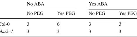
In total 56 metabolites were measured for 15 samples of Arabidosis wildtype seeds and 12 samples of aba2–1 mutant seeds. In Table 1, the number of samples for each combina-tion of genotypes (Col-0, aba2–1) and treatment (control or no treatment), −2.5 MPa polyethylene glycol (PEG), 5 μM Abscisic acid (ABA) or both (PEG+ABA) are given.
Table 1 Experimental design for plant data
Cell counts denote the number of samples obtained per combination of treatment and Genotype
No ABA Yes ABA
No PEG Yes PEG No PEG Yes PEG
Col-0 3 6 3 3
[image:5.595.309.544.629.693.2]To obtain the genotypic part of the metabolites we fit-ted Eq. 2 to the data where 𝐗m=𝐆 represents the geno-type; the four treatment levels were represented by two dummy variables denoting the administration of PEG and ABA. Thus, 𝐗(−m)= (𝐏𝐄𝐆,𝐀𝐁𝐀). Specifically for the pth
metabolite, the concentration associated with the seed’s genotype is given by:
Only significant variables were included in the models. Here we applied a hierarchical approach: if the highest order inter-action was significant, all terms were included in the model. If the highest order interaction was not significant it was removed from the model and the significance of the consecu-tive highest order interaction terms was checked. Finally if the genetic effect was not significant, the metabolite was dis-carded from further analysis. 48 metabolites were used for the network analysis of genotype related metabolic variation.
Hereafter we will denote networks of metabolites con-taining the original metabolite values (𝐘(p)) as
O and
net-works containing the genotype related values (𝐘̃(p)) as G.
(10) ̃
𝐘(p)=𝜷̂(p)
1 𝐆+𝜼̂ (p)
10𝐆◦𝐏𝐄𝐆+𝜼̂ (p)
01𝐆◦𝐀𝐁𝐀+𝜼̂ (p)
11𝐆◦𝐏𝐄𝐆◦𝐀𝐁𝐀.
3.1.1 Networks estimated by WGCNA
For estimation of the intensity matrix 𝐖 we first tried to find the soft thresholding parameter 𝛾 corresponding to a
scale free topology. However it appeared that for reasonable powers (𝛾 being <12) both networks (O and G) were not
scale-free. Therefore based on the sample size (N=27) and the number of metabolites (P=54 for O and P=48 for G), 𝛾 =5 was chosen for suppressing low correlations due
to noise (see Sect. 2.2.1).
In Fig. 2, the intensity matrices 𝐖O and 𝐖G are depicted together with their corresponding dendrograms obtained by average linkage hierarchical clustering. The visualization of the heatmaps reveals higher correlations (deeper red colors) between the genotype related metabolite values in (G) compared to the original metabolite values (O).
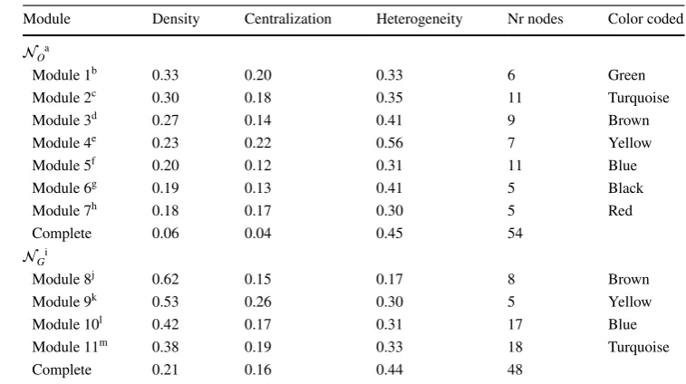
As seen in Table 2, the density and centralization of the complete networks are relatively low. The network G has a density of 0.21 and centralization of 0.16. The network
O has a density of 0.06 and a centralization of 0.04. With
regard to heterogeneity the two networks are similar (G
0.44 and O 0.45). The two most dense modules of G
have a moderate density of 0.62 and 0.53, but still small
Fig. 2 Heatmap plots for plant metabolites. Heatmaps were esti-mated for aO when the original metabolite values were used, and bG when using the metabolite information related to the Genotype. Deep red colors high values of absolute correlation between pairs of metabolites, while lighter colors correspond to weaker correlations.
[image:6.595.311.542.380.654.2]centralizations (0.15 and 0.26). The modules of O have
small densities, namely smaller than 0.33.
In Fig. 3, the top 5% of the strongest edges are visualized
for the network O and G. Here, a threshold of 0.36 for O and of 0.73 for G was used for keeping the top 5% of
the edges.
3.1.2 Networks estimated by GL
Next we consider the GL approach for estimation of net-works. The regularization parameter 𝜆 controlling the net-work’s sparsity was selected by using StARS (Liu et al. 2010). We randomly draw 100 subsamples of size 22 for estimating 𝜆. A disagreement allowance of 5%, gave a 𝜆O
of 0.82 and a 𝜆
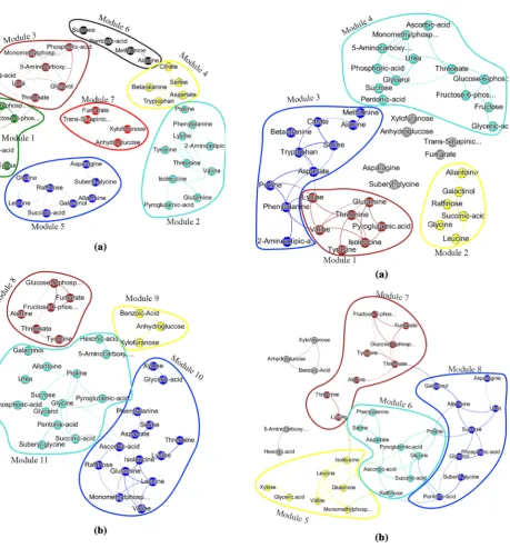
G of 0.94. In Fig. 4, the results are depicted.
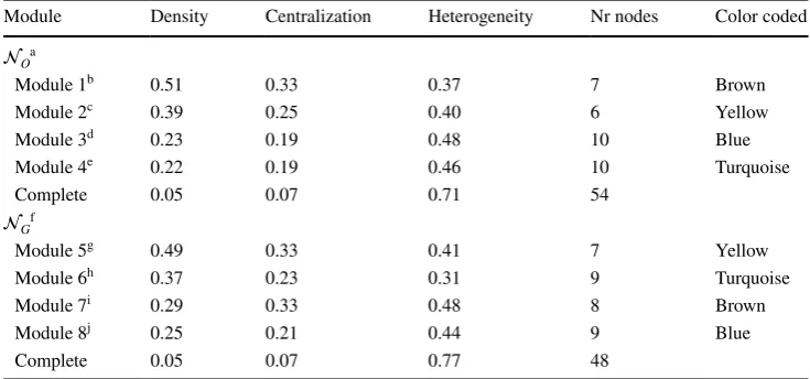
Here, the edges’ thickness and transparency denotes the edge’s stability i.e. frequency of edge occurrence in the 100 datasets. With regard to density, centralization and heter-ogeneity (Table 3) the two networks gave similar values. However, there was not much overlap between the identified modules of G and O obtained by the GL approach. Addi-tionally, there does not seem to be much overlap between the modules obtained by different network estimation methods (WGCNA vs. GL).
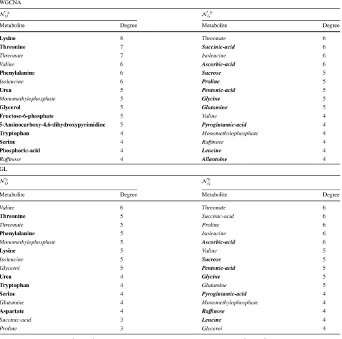
Top connected plant metabolites: In Table 4, the top con-nected plant metabolites for the O and G networks which were estimated by WGCNA or GL are given. In general, the GL approach yielded higher degrees of the metabolites for the G than for the O network. This was not the case
when the network was estimated by using WGCNA. Apart
Table 2 Network statistics when using WGCNA (density, centralization, heterogeneity) for modules and network as whole in plant data
a Network using the original metabolite values
b Module 1: fructose, fructose-6-phosphate, glucose, glucose-6-phosphate, glyceric-acid, xylose
c Module 2: 2-aminoadipic-acid, glutamine, isoleucine, lysine, nicotinic-acid, phenylalanine, proline,
pyro-glutamic-acid, threonine, tyrosine, valine
d Module 3: 5-aminocarboxy-4,6-dihydroxypyrimidine, ascorbic-acid, glutamate, glycerol, hexonic-acid,
monothylphosphate, phosphoric-acid, threonate, urea
e Module 4: aspartate, beta-alanine, citrate, ethanolamine, maltose, serine, tryptophan
f Module 5: alpha-ketoglutaric acid, allantoine, asparagine, fucose, galactinol, glycine, leucine, malate,
raf-finose , suberyl-glycine, succinic acid
g Module 6: alanine, methionine, myo-inositol, pentonic acid, sucrose
h Module 7: anhydroglucose, benzoic acid, fumarate, trans-sinapinic acid, xylofuranose i Network using genotypic-related information
j Module 8: alanine, fructose, fructose-6-phosphate, fumarate, glucose-6-phosphate, threonate,
trans-sinap-inic acid, tyrosine
k Module 9: 2-aminoadipic-acid, anhydroglucose, benzoic-acid, maltose, xylofuranose
l Module 10: ascorbic-acid, aspartate, glucose, glutamine, glyceric-acid, isoleucine, leucine, lysine,
raffi-nose, methionine, monomethylphosphate, phenylalanine, serine, threonine, tryptophan, valine, xylose
m Module 11: 5-aminocarboxy-4,6-dihydroxypyrimidine, allantoine, asparagine, citrate, galactinol, glycerol,
glycine, hexonic acid, malate, myo-inosytol, pentonic acid, phosphoric acid, proline, pyroglutamic acid, suberyl-glycine, succinic acid, sucrose, urea
Module Density Centralization Heterogeneity Nr nodes Color coded
Oa
Module 1b 0.33 0.20 0.33 6 Green
Module 2c 0.30 0.18 0.35 11 Turquoise
Module 3d 0.27 0.14 0.41 9 Brown
Module 4e 0.23 0.22 0.56 7 Yellow
Module 5f 0.20 0.12 0.31 11 Blue
Module 6g 0.19 0.13 0.41 5 Black
Module 7h 0.18 0.17 0.30 5 Red
Complete 0.06 0.04 0.45 54
Gi
Module 8j 0.62 0.15 0.17 8 Brown
Module 9k 0.53 0.26 0.30 5 Yellow
Module 10l 0.42 0.17 0.31 17 Blue
Module 11m 0.38 0.19 0.33 18 Turquoise
[image:7.595.166.545.55.267.2]from small differences, the two methods (WGCNA and GL) appeared to give similar lists of top connected metabo-lites but the order was different. Additionally, the top con-nected metabolites of G were different from the ones of
O in both WGCNA and GL cases. These results were also observed in Figs. 3 and 4.
3.2 Epidemiological study (DILGOM)
The other metabolomics dataset used has been measured in the epidemiological cohort DILGOM. A detailed description of the study and of the metabolomic dataset can be found in Inouye et al. (2010) and Kettunen et al. (2012). We excluded subjects who were diagnosed with diabetes, who received cholesterol medication, or who had outlying values for fast-ing glucose levels (>10 mmol/l). In addition only subjects with complete data were considered. After excluding these samples, we had 419 subjects (202 males and 217 females) aged between 25 and 74 years (median 53). The metabo-lomic data were measured by nuclear magnetic resonance (1H NMR) and comprise absolute quantitative measurements on 137 serum metabolites. Because of high correlation we
removed 78 lipid particle subfractions and only the total lipid concentrations per particle size were used. Addition-ally, one more metabolite (FALEN) was excluded since its measurements were not completely trusted. Our final dataset consisted of P=58 metabolites: 25 lipoproteins, 13 lipids
and fatty acids, 9 amino acids and 11 other small lites, e.g. involved in glycolysis. We adjusted all the metabo-lites for diastolic blood pressure (DBP) and blood pressure medication (BPM) (binary) by linear regression. In the rest of this section we will denote these adjusted metabolites as metabolites. We are interested in the network of metabolite concentrations and in the part of the metabolite concentra-tions related to BMI.
Since the metabolites and BMI depend on age and sex, these variables were included in model 2 as (𝐗1,𝐗2
) . The continuous BMI values were categorized into three equally sized classes (1st thirtile = 24.38, 2nd thirtile = 27.56). Thus in Eq. 2, the total number of covariables is m=3 and the
variable 𝐗3 represents the indicator variables for the three
BMI categories. The model 2 includes the main effects, first and second order interactions. Specifically for the pth metabolite, the following equation was used,
Table 3 Characterization of modules and network when estimating networks by GL and by using density, centralization and heterogeneity (edges’ stability has been used as weight) in plant data
a Network using the original metabolite values
b Module 1: glutamine, isoleucine, lysine, pyroglutamic acid, threonine, tyrosine, valine c Module 2: allantoine, galactinol, glycine, leucine, raffinose , succinic acid
d Module 3: 2-aminoadipic acid, alanine, aspartate, beta-alanine, citrate, methionine, phenylalanine, proline,
perine, tryptophan
e Module 4: 5-aminocarboxy-4,6-dihydroxypyrimidine, ascorbic acid, fructose, fructose-6-phospate,
glu-cose-6-phosphate, glyceric acid, glycerol, monomethylphosphate, pentonic acid, phosphoric acid, sucrose, threonate, urea
f Network using genotypic-related information
g Module 5: glutamine, glyceric acid, isoleucine, leucine, monomethylphosphate, valine, xylose
h Module 6: ascorbic-acid, aspartate, glycine, phenylalanine, proline, pyroglutamic acid, raffinose, serine,
succinic acid
i Module 7: alanine, fructose-6-phospate, fumarate, glucose-6-phosphate, lysine, threonate, threonine,
tyros-ine
j Module 8: allantoine, asparagine, galactinol, glycerol, pentonic acid, phosphoric acid, suberyl-glycine,
sucrose, urea
Module Density Centralization Heterogeneity Nr nodes Color coded
Oa
Module 1b 0.51 0.33 0.37 7 Brown
Module 2c 0.39 0.25 0.40 6 Yellow
Module 3d 0.23 0.19 0.48 10 Blue
Module 4e 0.22 0.19 0.46 10 Turquoise
Complete 0.05 0.07 0.71 54
Gf
Module 5g 0.49 0.33 0.41 7 Yellow
Module 6h 0.37 0.23 0.31 9 Turquoise
Module 7i 0.29 0.33 0.48 8 Brown
Module 8j 0.25 0.21 0.44 9 Blue
[image:8.595.177.545.58.230.2]Analogously to the plant application, networks of metabolites containing the original metabolite values
(
𝐘(p)) are denoted by O, and networks of metabolites containing the relevant information on BMI (𝐘̃(p)) by
B.
(11)
̃ 𝐘(p)
=𝜷̂(1p)𝐁𝐌𝐈+𝜼̂
(p)
10𝐁𝐌𝐈◦𝐀𝐠𝐞+𝜼̂
(p)
01𝐁𝐌𝐈◦𝐒𝐞𝐱
+𝜼̂(p)
11𝐁𝐌𝐈◦𝐀𝐠𝐞◦𝐒𝐞𝐱.
3.2.1 Networks estimated by WGCNA
For estimation of the intensity matrix, we first tried to deter-mine a soft-thresholding parameter 𝛾 for which the network
had a scale free topology. For both networks (the original and BMI related metabolite values), the scale-free topology
Fig. 3 Sparse plant metabolite networks estimated by WGCNA with
a the original metabolite values and b the Genotype related metabo-lite values. Modules have been color coded as indicated by column “Color Coded” in Table 2 in their corresponding network (O or G
). Colors have been selected by the two-step dynamic hybrid algo-rithm implemented in the R-package WGCNA
Fig. 4 Estimated metabolite networks for plant data based on GL. In
[image:9.595.81.541.47.541.2] [image:9.595.308.541.66.536.2]did not hold for reasonable powers, i.e. 𝛾 <12. Therefore, 𝛾 =3 was chosen based on the sample size (n=419) and the
number of metabolites (P=58) as described in Sect. 2.2.1.
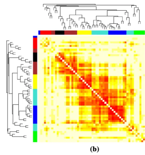
The absolute values of Pearson’s correlation coefficients are visualized in Fig. 5; darker red colors represent strong cor-relations, and lighter colors weaker correlations. The heat-map of B shows several larger blocks of highly correlated
metabolites while the heatmap of O shows several small
and distinct clusters.
For visualizing and depicting edges in both networks we used the following thresholds: 0.22 for O and 0.66
for B. These thresholds correspond to the top 10% of the
edges (Fig. 6). For identifying interconnected modules, we applied average linkage hierarchical clustering and obtained
Table 4 List of top connected plant metabolites for network estimation using WGCNA and GL
Results are displayed for the O and G networks. Italic denotes that the metabolite appears in both O and G networks. Bold is for
metabo-lites that appear only in the list of O network and bolditalic for metabolites that appear only in the list of the G network
a
O network using the original metabolite values
b
G network using genotypic-related information
WGCNA
Oa Gb
Metabolite Degree Metabolite Degree
Lysine 8 Threonate 6
Threonine 7 Succinic-acid 6
Threonate 7 Isoleucine 6
Valine 6 Ascorbic-acid 6
Phenylalanine 6 Sucrose 5
Isoleucine 6 Proline 5
Urea 5 Pentonic-acid 5
Monomethylophosphate 5 Glycine 5
Glycerol 5 Glutamine 5
Fructose‑6‑phosphate 5 Valine 4
5‑Aminocarboxy‑4,6‑dihydroxypyrimidine 5 Pyroglutamic-acid 4
Tryptophan 4 Monomethylophosphate 4
Serine 4 Raffinose 4
Phosphoric‑acid 4 Leucine 4
Raffinose 4 Allantoine 4
GL a
O
b
G
Metabolite Degree Metabolite Degree
Valine 6 Threonate 6
Threonine 5 Succinic‑acid 6
Threonate 5 Proline 6
Phenylalanine 5 Isoleucine 6
Monomethylophosphate 5 Ascorbic-acid 6
Lysine 5 Valine 5
Isoleucine 5 Sucrose 5
Glycerol 5 Pentonic-acid 5
Urea 4 Glycine 5
Tryptophan 4 Glutamine 5
Serine 4 Pyroglutamic-acid 4
Glutamine 4 Monomethylophosphate 4
Aspartate 4 Raffinose 4
Succinic‑acid 3 Leucine 4
[image:10.595.52.547.75.565.2]dendograms. Modules were defined as branches of the den-dogram and were identified using the two-step dynamic hybrid algorithm. The descriptives of the two networks are given in Table 5. The complete network B has a larger
density (0.23 vs. 0.07) and centralization (0.17 vs. 0.11) and a lower heterogeneity value (0.50 vs. 0.76) than the complete network O. The first three modules of B are more dense
than the modules of NO (0.63–0.77 vs. 0.15–0.32). The
cen-tralization and the heterogeneity of the modules of NG are smaller than of the modules of NO. In both cases, centraliza-tion exhibits relatively low values denoting that there is not a dominant metabolite in each of the modules.
3.2.2 Networks estimated by GL
Next we considered the GL approach. The penalty parameter 𝜆 was selected by using StARS (Liu et al. 2010). We used a size for the subsamples of 205 (almost 50% of the total
sample size) and a disagreement allowance of 2% across the
networks. After subsampling 100 times, we obtained a 𝜆O
of 0.68 and 𝜆B of 0.91. Fig. 7 depicts the results. Here the edge thickness represent the stability of the estimated edges. The evaluation measures are also calculated based on stabil-ity (Table 6). The densstabil-ity, centralization, and heterogenestabil-ity was very similar for both networks. The first modules of each network contained exactly the same metabolites and
had also very similar properties. Interestingly the second dense module of G (VLDL) and third of the O (BCAA/
VLDL) had a large overlap with regard to VLDL parti-cles. Note that VLDL particles were also identified by the WGCNA approach as a module. In Fig. 1 metabolite con-centrations stratified by BMI and Sex are depicted for the VLDL module. It appeared that all these eight metabolites had a high value in obese men. For females the values were much lower for these metabolites except for alanine. Note that alanine is also on the border of the cluster (Figs. 6b, 7b) and shares connections with metabolites from other mod-ules. Finally, the third densest module in B (FA) identified
by GL exhibits a relatively high centralization. This denotes that some metabolite(s) had higher than average degree (hub metabolite(s)). The metabolite with the highest strength (6.99) and degree (7) as measured by the stability in GL within the module is monounsaturated fatty acids (MUFA). MUFA being connected to all metabolites in the FA module (only pyruvate is not a direct connection) indicates that it might have the most representative metabolite profile among the rest. LLDLL (total lipids of large LDL particles), with eight connections and strength 7.98 is the metabolite with the most connections within the Lipoproteins module. In the VLDL module, LVLDLL has the most connections (six connections) with strength of 5.98.
Fig. 5 Correlation matrix plot. The plots were generated for aO
using the original metabolite values, and bB using BMI informa-tion. Dendrograms were obtained by ordering metabolites using hierarchical clustering. Modules of interconnected metabolites cor-respond to square blocks along the diagonal, while deep red colors
[image:11.595.295.540.52.314.2]Top connected metabolites In Table 7 the top 15 metab-olites are given for combinations of the two approaches (WGCNA and GL) and two types of correlation structures (metabolites and BMI specific metabolites). The degree k of the metabolites was higher for WGCNA than for GL. The same conclusion holds when comparing Figs. 6b, 7b.
4 Discussion
In this paper we studied and visualized the correlation structure of two datasets of metabolomics coming from two different studies. The studies differ in types of subjects, study designs and sizes. We considered two methodologi-cal approaches to estimate the networks: namely WGCNA based on correlation and GL based on partial correlation. The methods were applied to the metabolite values and to parts of the metabolite values which incorporate the effect of a covariable of interest, e.g. genotype or BMI. We compared the obtained networks in terms of density, centralization and heterogeneity of the relationships between the nodes.
The density of the networks based on the covariable spe-cific part of the metabolites had larger or similar values than the density of the networks based on the metabolites itself. Interestingly, for the metabolites measured in the epidemio-logical study, a number of lipoproteins (i.e. IDLC, IDLL, LDLC, LLDLL, SERUMC, SLDLL, SM, XSVLDLL) was clustered together when keeping the original or the BMI-spe-cific metabolite values in both network estimation methods. In addition, for the BMI specific part both approaches iden-tified exactly the same module consisting mainly of VLDL particles with a density of 0.77 using Pearson correlation, and a density of 0.61 using stability in the GL approach. This module is characterized by high values for obese men. The relationship between BMI and VLDL concentrations is known. In several studies it has been found that obese people have elevated VLDL concentrations (almost by 50%; Magkos et al. 2008) compared to lean individuals (Mitten-dorfer et al. 2003; Chan et al. 2004; Goff et al. 2005; Mag-kos et al. 2008; MagMag-kos and Mittendorfer 2009). This can be attributed to the hepatic overproduction of VLDL parti-cles (Chan et al. 2004; Ooi et al. 2005) which characterizes
Table 5 Characterization of modules and network in humans with WGCNA using density, centralization and heterogeneity
a Network using the original metabolite values
b FA/LDL: APOB, DHA, FAW3, FAW3FA, FAW6,IDLC, IDLL, LA, LDLC, LLDLL, MLDLL, PC,
SERUMC, SLDLL, SM, TOTPG, XSVLDLL
c HDL: ALB, APOA1, HDL2C, HDLC, LHDLL, MHDLL, SHDLL, XLHDLL
d VLDL/AA: ALA, FAW6FA, GLC, GP, HDL3C, ILE, LAC, LDLD, LEU, LVLDLL, MUFA, MVLDLL,
PHE, PYR, SERUMTG, SVLDLL, TOTFA, TYR, VAL, VLDLD, XLVLDLL, XXLVLDLL
e Network using BMI-related information
f VLDL: ALA, LVLDLL, MVLDLL, SERUMTG, SVLDLL, VLDLD, XLVLDLL, XXLVLDLL g HDL: ACACE, APOA1, BOHBUT, HDL2C, HDLC
h IDL/LDL: ACE, IDLC, IDLL, LDLC, LEU, LLDLL, MLDLL, SERUMC, SLDLL, SM, XSVLDLL i FA/lipids: APOB, FAW3FA, FAW6, GLOL, LA, LAC, LDLD, MUFA, PC, PYR, SHDLL, TOTFA,
TOTPG
j FA/others: GLC, GP, HDLD, ILE, LHDLL, PHE, TYR, VAL, XLHDLL k FA: CIT, DHA, FAW3, FAW6FA, GLN, MHDLL
l AA/lipoproteins: ALB, CREA, GLY, HDL3C, HIS, UREA
Module Density Centralization Heterogeneity Nr nodes Color coded
Oa
FA/LDLb 0.32 0.19 0.45 17 Blue
HDLc 0.31 0.23 0.55 9 Brown
VLDL/AAd 0.15 0.19 0.72 22 Turquoise
Complete 0.07 0.11 0.76 58
Bb
VLDLe 0.77 0.11 0.11 8 Yellow
HDLg 0.67 0.15 0.15 5 Black
LDL/IDLh 0.63 0.18 0.35 11 Blue
FA/lipidsi 0.59 0.16 0.19 13 Turquoise
FA/othersj 0.54 0.15 0.27 9 Brown
FAk 0.20 0.20 0.42 6 Green
AA/lipoproteinsl 0.19 0.16 0.38 6 Red
[image:12.595.180.543.58.255.2]obesity. Hepatic overproduction of VLDL particles is also stimulated by atherogenic dislipidemia (which is commonly present in obese people) and promoted by increased liver fat (Grundy 2004; Klop et al. 2013), also common in obese people. Finally, abdominal fat (known as visceral adipose tissue) and BMI have been found to be positively associated to VLDL particle concentrations and size suggesting again the association between obesity and high levels of VLDL (Sam et al. 2008).
The results for the data from the Arabidopsis desicca-tion tolerance experiments were harder to interpret. In general, the densities and centralizations of the networks were smaller. This might be the result of the small sample size. Indeed the 𝛾 parameter to shrink small values in the
WGCNA approach is larger for the experimental than for the epidemiological design (five and three respectively). However for the GL approach there was less difference in the shrinkage, namely the shrinkage parameter was 0.68 and 0.91 for NO and NB in the epidemiology study and 0.82 and
0.94 for NO and NG in the experimental design. While in the
epidemiological study the network specific to BMI provided interesting results, this was less the case for the desiccation tolerance data. One reason may be that the main effect of the genotype on the metabolite variation was smaller than the main effect of the treatment. We presented a treatment corrected metabolic network reconstrution in which the wild type and mutant type genotypes are compared across
treatments. This is a sensible analysis in plant genetics (Eeuwijk et al. 2010). However, from a seed physiological perspective an analysis correcting for genotype and compar-ing the treatments across the two genotypes may be more interesting. We will present the results of such an analysis elsewhere.
WGCNA and GL are complementary approaches for metabolite inference since the former recovers meaningful modules and the latter recovers meaningful edges, e.g. for the DILGOM study MUFA is the dominant metabolite in the FA module when GL is used. WGCNA is based on the correlation structure, and the obtained results are therefore straightforward to interpret. To reduce the noise in the data, a soft threshold is often applied to sufficiently shrink small correlations to zero. WGCNA allows detection of modules with high density. GL is based on Gaussian graphical mod-els, in which the conditional independence is inferred by the zero entries in the precision matrix. In order to induce sparsity to the precision matrix and to estimate stable sets of edges with a low false discovery rate, a stability selection approach, StARS, was applied. This can lead to detection of modules with high centralization. For both approaches modules are selected by constructing a dendogram based on average linkage and cutting the branches.
In both cases, WGCNA and GL, the user has to choose specific tuning parameters: the soft threshold in WGCNA and the disagreement allowance and the number of the
Table 6 Characterization of modules and network in GL using density, centralization and heterogeneity (edges stability has been used as weight) in humans
a Network using the original metabolite values
b LDL/IDL: IDLC, IDLL, LDLC, LLDLL, MLDLL, SERUMC, SLDLL, SM, XSVLDLL c FA: APOB, FAW6, LA, MUFA, SVLDLL, TOTFA
d BCAA/VLDL: ILE, LEU, LVLDLL, MVLDLL, SERUMTG, VAL, VLDLD, XLVLDLL, XXLVLDLL e HDL: APOA1, HDL2C, HDLC, HDLD, LHDLL, MHDLL, PC, TOTPG, XLHDLL
f Network using BMI-related information
g LDL/IDL: IDLC, IDLL, LDLC, LLDLL, MLDLL, SERUMC, SLDLL, SM, XSVLDLL h VLDL: ALA, LVLDLL, MVLDLL, SERUMTG, SVLDLL, VLDLD, XLVLDLL, XXLVLDLL i FA: APOB, FAW6, LA, LAC, MUFA, PC, PYR, TOTFA, TOTPG
j Lipids/HDL: ACACE, BOHBUT, GP, HDL2C, HDLC, HDLD, ILE, LHDLL, PHE, XLHDLL
Module Density Centralization Heterogeneity Nr nodes Color coded
Oa
LDL/IDLb 0.71 0.31 0.34 9 Blue
FAc 0.65 0.45 0.28 6 Yellow
BCAA/VLDLd 0.56 0.23 0.38 9 Turquoise
HDLe 0.45 0.27 0.45 6 Brown
Complete 0.07 0.17 0.98 58
Bf
LDL/IDLg 0.79 0.27 0.24 9 Blue
VLDLh 0.61 0.30 0.35 8 Yellow
FAi 0.44 0.56 0.45 9 Brown
Lipids/HDLj 0.30 0.31 0.42 10 Turquoise
[image:13.595.170.544.54.230.2]subsamples for GL with StARS. For a large dataset, StARS might not be needed and the penalty parameter might be chosen based on cross validation making the procedure to be data driven. The impact of the tuning parameters in WGCNA and GL is high; so data driven methods for selecting them would be ideal.
For clear visualization of the constructed networks using WGCNA, arbitrary thresholds were applied to depict the top 5% of the edges in the experimental design and 10% in
the human data. These numbers were selected together with plant biologists and epidemiologists so that a set of mean-ingful edges was recovered by the data. The disagreement allowance parameter in GL was set to 5% in the experimental Fig. 6 Estimated sparse metabolite networks in humans based on
WGCNA. In a, the network is based on the original metabolite val-ues. In b the BMI related metabolite network is displayed. Metabo-lites have been colored by the color of the module they belong to. Information on the color of each module can be found in Table 5.
Colors were selected based on the two-step dynamic hybrid algorithm
[image:14.595.62.326.52.500.2] [image:14.595.186.524.53.561.2]design and 2% in the epidemiological data for the same
reason.
Apart from the two considered methods for estimating networks of metabolites, other well established methods have been used in practice based on conditional independ-ence using regression techniques, ridge regularization and partial correlation. First, a simple approach for estimating
sparse networks using regression techniques is by estimat-ing the edge set for each variable by fittestimat-ing a Lasso model to each variable using the remaining variables as predic-tors (Meinshausen and Bühlmann 2006). The non-zero Lasso coefficients identify the adjacent nodes to which each variable is connected to. The shortcoming of this method compared to GL which estimates the network structure
Table 7 List of top connected plant metabolites for network estimation using WGCNA and GL
Results are displayed for the O and G networks. Italic denotes that the metabolite appears in both O and G networks. Bold is for metabo-lites that appear only in the list of O network and Bolditalic for metabolites that appear only in the list of the G network
a Network using the original metabolite values b Network using BMI-related information
WGCNA
Oa Bb
Metabolite Degree Metabolite Degree
TOTFA 16 TOTFA 17
FAW6 16 SVLDLL 15
APOB 15 APOB 15
SVLDLL 14 SERUMTG 14
SERUMC 14 SLDLL 14
LA 14 FAW6 14
MUFA 14 MLDLL 12
XSVLDLL 12 MUFA 12
MLDLL 12 ALA 11
SLDLL 12 LVLDLL 10
SERUMTG 12 MVLDLL 10
MVLDLL 11 XSVLDLL 10
IDLL 11 XLVLDLL 9
LLDLL 11 IDLL 9
IDLC 11 ILE 9
GL
Oa Bb
Metabolite Degree Metabolite Degree
APOB 13 LLDLL 9
SERUMC 12 MLDLL 9
SERUMTG 10 APOB 9
TOTFA 10 SVLDLL 8
LVLDLL 9 IDLL 8
MVLDLL 9 LDLC 8
LLDLL 9 SERUMTG 8
MLDLL 9 SLDLL 7
SLDLL 9 IDLC 7
IDLC 9 SERUMC 7
XLVLDLL 8 FAW6 7
IDLL 8 TOTFA 7
LDLC 8 MUFA 7
FAW6 8 LVLDLL 6
[image:15.595.52.547.75.556.2]simultaneously, is that an edge between two nodes (p and
q) might be estimated from p to q but not vice versa. For overcoming this, an AND or an OR rule can be applied. This method asymptotically estimates the set of non zero ele-ments of the precision matrix, but it does not yield the maxi-mum likelihood estimator (Banerjee et al. 2008). In contrast to Lasso penalty in GL which estimates entries in the pre-cision matrix (and subsequently in the adjacency matrix) exactly equal to zero, a ridge penalty can also be used in the penalized log likelihood (Ha and Sun 2014). The elements in the precision matrix will shrink, but will not be exactly zero unless a threshold is chosen for having exactly zeros (Efron 2004). In this case, GL seems to be advantageous due to the sparsity that is preferred for interpreting the results. Also, by applying a threshold in the ridge-based method, a second parameter should be estimated on top of the ridge penalty 𝜆ridge. This usually involves a two-dimensional grid
search approach that can be time-consuming and the opti-mization problem might not be convex as well. Finally, the edges of the network can be chosen by estimating Pearson’s partial correlation coefficient for any given pair of variables directly. Partial correlation eliminates edges that appear from indirect effects which is a desired characteristic (Krum-siek et al. 2011). The shortcoming of the method is that it is not applicable in the high dimensional setting. In this case, partial correlation cannot be estimated by either using the linear regression, or the matrix inversion methods. Using a recursive formula is also not possible and is computation-ally expensive. Therefore, here we used WGCNA which is a commonly used approach and is based on observed cor-relations which are easy to interpret. GL is also used since it has all desirable features (sparsity, computational speed, can be used in high-dimensional setting) that the other methods fall short of.
For identifying and selecting modules in this paper, the two-step dynamic hybrid algorithm was used with 1−wij as a dissimilarity measure in WGCNA and one minus stabil-ity of the edges (number of edges occurrences from the subsampling scheme) in GL. Another popular clustering method is the modularity optimization. Dividing a network in modules so that the modularity is optimal, will result in many edges within the modules and few edges between modules (Newman and Girvan 2004). Module identifica-tion by using modularity optimizaidentifica-tion is a known data-driven approach, which is used without specifying any arbitrary parameters. Here the dynamic hybrid algorithm was used instead, because while it takes the modular struc-ture into account (through the dendrogram), it additionally does not have a constant cut-off height, so is able to iden-tify nested clusters by using the cluster shape.
Some issues still need to be addressed. For example network estimation methods should thoroughly be investi-gated on the sample size sensitivity (large vs. small sample
sizes) and in changes on tuning parameters (soft-threshold in WGCNA, disagreement allowance in GL). Further work for repeated measurements of the metabolites over time should be considered.
The regression framework to study specific parts of the metabolite concentrations worked well for the epidemio-logical dataset. We recovered sets of metabolites that are associated to a categorical covariable of interest in the same way. By using a network approach coupled with a module identification method, sets of metabolites which regulate the covariable of interest in the same way can be detected.
Acknowledgements We thank Markus Perola and Perttu Salo from the National Institute for Health and Welfare (THL) for their discus-sions and Yrjö Jahnsson Foundation for the DILGOM NMR data.
Funding This study was funded by the European Union’s Seventh Framework Program (FP7-Health-F5-2012) under Grant Agreement Number 305280 (MIMOmics).
Compliance with ethical standards
Conflict of interest All the author’s declare that they have no con-flict of interest.
Ethical approval All participants gave written informed consent, and the human study has local ethical committee approval [the ethics committee of Helsinki University Hospital, Finland (IRB00003181), for DILGOM (229/E0/2006)]. This article does not contain any studies with animals performed by any of the authors.
Open Access This article is distributed under the terms of the Creative Commons Attribution 4.0 International License (
http://crea-tivecommons.org/licenses/by/4.0/), which permits unrestricted use,
distribution, and reproduction in any medium, provided you give appro-priate credit to the original author(s) and the source, provide a link to the Creative Commons license, and indicate if changes were made.
References
Banerjee, O., Ghaoui, L. E., & d’Aspremont, A. (2008). Model selec-tion through sparse maximum likelihood estimaselec-tion for multi-variate gaussian or binary data. Journal of Machine Learning Research, 9, 485–516.
Chan, D. C., Barrett, H. P., & Watts, G. F. (2004). Dyslipidemia in visceral obesity. American Journal of Cardiovascular Drugs,
4(4), 227–246.
DiLeo, M. V., Strahan, G. D., den Bakker, M., & Hoekenga, O. A. (2011). Weighted correlation network analysis (WGCNA) applied to the tomato fruit metabolome. PLoS ONE, 6(10), e26683.
Dong, J., & Horvath, S. (2007). Understanding network concepts in modules. BMC Systems Biology, 1(1), 24.
Efron, B. (2004). Large-scale simultaneous hypothesis testing: The choice of a null hypothesis. Journal of the American Statistical Association, 99(465), 96–104.
Friedman, J., Hastie, T., & Tibshirani, R. (2008). Sparse inverse covariance estimation with the graphical lasso. Biostatistics, 9(3), 432–441.
Goff, D. C., D’Agostino, R. B., Haffner, S. M., & Otvos, J. D. (2005). Insulin resistance and adiposity influence lipoprotein size and subclass concentrations. results from the insulin resistance ath-erosclerosis study. Metabolism, 54(2), 264–270.
Grundy, S. M. (2004). Obesity, metabolic syndrome, and cardiovascu-lar disease. The Journal of Clinical Endocrinology & Metabolism,
89(6), 2595–2600.
Ha, M., & Sun, W. (2014). Partial correlation matrix estimation using ridge penalty followed by thresholding and re-estimation. Biom‑ etrics, 70(3), 762–770.
Hastie, T., Tibshirani, R., & Friedman, J. (2009). Unsupervised learn‑ ing. New York: Springer.
Horvath, S., & Dong, J. (2008). Geometric interpretation of gene coex-pression network analysis. PLoS Computational Biology, 4(8), e1000117.
Inouye, M., Kettunen, J., Soininen, P., Silander, K., Ripatti, S., Kum-pula, L. S., et al. (2010). Metabonomic, transcriptomic, and genomic variation of a population cohort. Molecular Systems Biology, 6(1), 441.
Kettunen, J., Tukiainen, T., Sarin, A.-P., Ortega-Alonso, A., Tikkanen, E., Lyytikäinen, L.-P., et al. (2012). Genome-wide association study identifies multiple loci influencing human serum metabolite levels. Nature Genetics, 44(3), 269–276.
Klop, B., Elte, J. W. F., & Cabezas, M. C. (2013). Dyslipidemia in obesity: Mechanisms and potential targets. Nutrients, 5(4), 1218–1240.
Kolaczyk, E. D., & Krivitsky, P. N. (2015). On the question of effective sample size in network modeling: An asymptotic inquiry. Statisti‑ cal Science: A Review Journal of the Institute of Mathematical Statistics, 30(2), 184.
Krumsiek, J., Suhre, K., Illig, T., Adamski, J., & Theis, F. (2011). Gaussian graphical modeling reconstructs pathway reactions from high-throughput metabolomics data. BMC Systems Biology, 5(1), 21.
Langfelder, P., & Horvath, S. (2008). WGCNA: An R package for weighted correlation network analysis. BMC Bioinformatics, 9(1), 559.
Langfelder, P., Zhang, B., & Horvath, S. (2008). Defining clusters from a hierarchical cluster tree: The dynamic tree cut package for R.
Bioinformatics, 24(5), 719–720.
Lauritzen, S. L. (1996). Graphical models. Oxford: Clarendon Press. Liu, H., Roeder, K. & Wasserman, L. (2010). Stability approach to
regularization selection (stars) for high dimensional graphical models. In Advances in neural information processing systems
(pp. 1432–1440).
Magkos, F., & Mittendorfer, B. (2009). Gender differences in lipid metabolism and the effect of obesity. Obstetrics and Gynecology Clinics of North America, 36(2), 245–265.
Magkos, F., Mohammed, B. S., & Mittendorfer, B. (2008). Effect of obesity on the plasma lipoprotein subclass profile in
normoglycemic and normolipidemic men and women. Interna‑ tional Journal of Obesity, 32(11), 1655–1664.
Maia, J., Dekkers, B. J., Dolle, M. J., Ligterink, W., & Hilhorst, H. W. (2014). Abscisic acid (aba) sensitivity regulates desiccation toler-ance in germinated arabidopsis seeds. New Phytologist, 203(1), 81–93.
Maia, J., Dekkers, B. J., Provart, N. J., Ligterink, W., & Hilhorst, H. W. (2011). The re-establishment of desiccation tolerance in germi-nated arabidopsis thaliana seeds and its associated transcriptome.
PLoS ONE, 6(12), e29123.
Meinshausen, N., & Bühlmann, P. (2006). High-dimensional graphs and variable selection with the lasso. The Annals of Statistics,
34(1), 1436–1462.
Mittendorfer, B., Patterson, B. W., & Klein, S. (2003). Effect of sex and obesity on basal VLDL-triacylglycerol kinetics. The American Journal of Clinical Nutrition, 77(3), 573–579.
Newman, M. E., & Girvan, M. (2004). Finding and evaluating com-munity structure in networks. Physical Review E, 69(2), 026113. Ooi, E. M., Watts, G. F., Farvid, M. S., Chan, D. C., Allen, M. C.,
Zilko, S. R., et al. (2005). High-density lipoprotein apolipoprotein A-I kinetics in obesity. Obesity Research, 13(6), 1008–1016. Rothman, A. J., Bickel, P. J., Levina, E., Zhu, J., et al. (2008). Sparse
permutation invariant covariance estimation. Electronic Journal of Statistics, 2, 494–515.
Sam, S., Haffner, S., Davidson, M. H., D’Agostino, R. B., Feinstein, S., Kondos, G., et al. (2008). Relationship of abdominal visceral and subcutaneous adipose tissue with lipoprotein particle number and size in type 2 diabetes. Diabetes, 57(8), 2022–2027.
van Eeuwijk, F. A., Bink, M. C., Chenu, K., & Chapman, S. C. (2010). Detection and use of QTL for complex traits in multiple environ-ments. Current Opinion in Plant Biology, 13(2), 193–205. Yuan, M., & Lin, Y. (2006). Model selection and estimation in
regres-sion with grouped variables. Journal of the Royal Statistical Soci‑ ety: Series B (Statistical Methodology), 68(1), 49–67.
Zhang, B., & Horvath, S. (2005). A general framework for weighted gene co-expression network analysis. Statistical Applica‑ tions in Genetics and Molecular Biology, 4(1). https://doi.
org/10.2202/1544-6115.1128.
Zhang, G., He, P., Tan, H., Budhu, A., Gaedcke, J., Ghadimi, B. M., et al. (2013). Integration of metabolomics and transcriptomics revealed a fatty acid network exerting growth inhibitory effects in human pancreatic cancer. Clinical Cancer Research, 19(18), 4983–4993.
Zhao, T., Liu, H., Roeder, K., Lafferty, J., & Wasserman, L. (2012). The huge package for high-dimensional undirected graph esti-mation in R. The Journal of Machine Learning Research, 13(1), 1059–1062.