Inducing protein aggregation by extensional flow

This is a repository copy of Inducing protein aggregation by extensional flow. White Rose Research Online URL for this paper:

http://eprints.whiterose.ac.uk/114410/ Version: Supplemental Material

Article:

Dobson, J, Kumar, A, Willis, LF orcid.org/0000-0001-6616-3716 et al. (8 more authors) (2017) Inducing protein aggregation by extensional flow. Proceedings of the National Academy of Sciences, 114 (18). pp. 4673-4678. ISSN 1091-6490

https://doi.org/10.1073/pnas.1702724114

This article is protected by copyright. All rights reserved. This is an author produced version of a paper published in the Proceedings of the National Academy of Sciences. Uploaded in accordance with the publisher's self-archiving policy. In order to comply with the publisher requirements the University does not require the author to sign a

non-exclusive licence for this paper.

[email protected] https://eprints.whiterose.ac.uk/ Reuse

Unless indicated otherwise, fulltext items are protected by copyright with all rights reserved. The copyright exception in section 29 of the Copyright, Designs and Patents Act 1988 allows the making of a single copy solely for the purpose of non-commercial research or private study within the limits of fair dealing. The publisher or other rights-holder may allow further reproduction and re-use of this version - refer to the White Rose Research Online record for this item. Where records identify the publisher as the copyright holder, users can verify any specific terms of use on the publisher’s website.

Takedown

If you consider content in White Rose Research Online to be in breach of UK law, please notify us by

1

Supplementary information

1

2

Inducing protein aggregation by extensional flow

3

4

John Dobson, Amit Kumar, Leon F. Willis, Roman Tuma, Daniel R. Higazi, Richard Turner, 5

David Lowe, Alison E. Ashcroft, Sheena E. Radford, Nikil Kapur, and David J. Brockwell 6

7

8

9

2 Supplementary method 1 2 CFD 3

The CFD package used for this study is COMSOL 4.3b which employs a finite element method. 4

The fluid properties used in the model were those of water at 20 °C (predefined within the CFD 5

package) as protein solutions were prepared at low enough concentrations so as to have 6

negligable effect on fluid viscosity (1). The pertinent geometry of the constriction region where 7

the extensional flow field occurs is shown Figure 1 in three-dimensions; judicious choice of 8

boundary conditions allows this to be modelled as a 2-dimensional slice in an axial co-ordinate 9

system (Figure 1 D(i)) without the loss of any of the underlying physics but with the advantage 10

of reducing the scale of the computational problem. The inlet is specified as a fully developed 11

laminar flow (flow through the device is slow with low Reynolds number, Re<<2000, see 12

below) with a specified volumetric flow rate that is chosen to match that created by the piston 13

movement within the syringe body. The outlet is defined as a pressure condition, and is located 14

far enough downstream of the constriction to prevent back-flow into the domain. The bottom 15

edge of the domain represents the axis of symmetry of the problem and the axis about which 16

the slice is rotated about to give the fully reconstructed domain. Axial symmetry was defined 17

about the radial axis r = 0. A no slip boundary condition was enforced on all of the remaining 18

vertices in the model. The mesh was a relatively fine quadrilateral mesh with uniform finite 19

elements making up the main bulk of the model and finer elements at the walls to give accurate 20

non-slip boundary conditions. Lack of sensitivity of the solution to the mesh was confirmed. 21

22

The general steps of defining the geometry (using the parameters shown in Table S1), applying 23

boundary conditions, discretising the domain into a grid structure and solving the flow field 24

3

accurately. From a characterization perspective, the laminar Navier-Stokes equations in an axi-1

symmetric coordinate system are solved to characterize the flow in terms of the velocity and 2

pressure at each point, which can then be interpreted in terms of the shearing and extensional 3

flow field. The flow exponent (Q = k∆Pn, where Q is the flow rate, is the pressure drop 4

and k is the flow coefficient of units m3s-1Pan) was calculated to determine the dominant flow 5

regime; where n =1 is laminar and n = 0.5 is turbulent. For our device, n = 0.905 and thus 6

generates a predominantly laminar flow. In accordance with this, the Reynolds Number was 7

found to be <<2000 throughout the device (Table S1). 8

9

Reynolds number

10

Reynolds number was calculated by: 11

12

Where is the fluid density, u the fluid velocity, L a characteristic length scale (in this case the 13

pipe diameter) and µ is the dynamic viscosity. 14

Extensional flow

15

Strain is a measure of mechanical extension given by where is the original length 16

and is the extended length. Therefore rate of strain is the time derivative of . Along the 17

axis the centre-line strain is given by . More generally, the strain rate field is 18

calculated following the deformation tensors described in (2) 19

20

4

Calculating Hydraulic Energy

1

The energy applied to a unit sphere as it passes through the contraction is calculated as 2

where is the sphere volume, is the volumetric flow rate and is the hydraulic power. 3

The hydraulic power is calculated from where is either the pressure drop over 4

the contraction or capillary. The pressure drop is taken from the CFD simulation. 5

6

Model used to estimate extensional force

7

The force applied onto a protein molecule was estimated using the “elementary model for shear 8

denaturation of a protein by elongational flow” (Figure 7, ref (3)). The protein model used in 9

our calculations comprised 583 residues configured as a dumbbell of two spheres each 10

containing 2/5 of the residues, joined by the remaining residues in an extended conformation. 11

12

Operation of extensional flow device

13

The syringes were aligned and secured using a ThorLabs optics board. A screw-jack linear 14

actuator attached to two shunts was used to depress the syringe plungers. The actuator was 15

driven by a single stepper motor to allow for accurate flow rate and volume control. 16

The protein solution was shuttled between the two syringes along the capillary tube as seen in 17

(Figure 1). The syringe plungers are linked hydraulically through the protein solution such that, 18

as one syringe plunger is depressed, the fluid forces cause the other to be expelled from its 19

syringe jacket. The stepper motor was controlled directly by an embedded microcontroller 20

maintaining a constant velocity throughout the experiment. Prior to each experiment, the 21

syringes were flushed with 2 % (v/v) Hellmanex-III solution and MilliQ-grade H2O, followed

5

by a final wash with 0.22 µm-filtered and de-gassed buffer. 500 L of 0.22 µm-filtered protein 1

solution was drawn into one syringe very slowly through the capillary so as not to damage the 2

protein prematurely. Any bubbles were expelled and then the other end of the capillary attached 3

to the second empty syringe (pre-secured to the optics board with the plunger fully depressed 4

to eliminate air from the system), sealed with the compression fitting and the first syringe 5

clamped in place. 6

7

Purification of GCSF C3

8

Cell pellets were resuspended in lysis buffer (50 mM TrisHCl, 5 mM EDTA, 2 mM 9

phenylmethanesulphonyl fluoride (PMSF) and 2 mM benzamidine hydrochloride hydrate pH 10

8) at a ratio of 1 g of cell pellet to 10 mL of buffer and lysed by 5× 30 second periods of 11

sonication on ice at 75 % amplitude, using a Sonics Vibra-CellTM _{VCX-130PB sonicator with}

12

a 6 mm diameter probe. Inclusion bodies were harvested by centrifugation at 15000 rpm, 4 °C 13

for 30 mins, using a Beckman Coulter Avanti J-26 XP centrifuge with JLA 16.250 rotor. 14

Inclusion bodies were then washed by re-suspending in wash buffer 1 (50 mM TrisHCl, 5 mM 15

EDTA, 1 % (v/v) triton X-100 pH 8) at a ratio of 1 g of inclusion body pellet to 20 mL of buffer 16

and harvesting inclusion bodies by centrifugation as before. This wash step was repeated using 17

wash buffer 2 (50 mM TrisHCl, 5 mM EDTA, 4 M urea pH 8). Washed inclusion bodies were 18

resuspended in unfolding buffer (50 mM TrisHCl, 5 mM EDTA, 6 M GdnHCl, 10 mM DTT 19

pH 8) at a ratio of 1 g of inclusion body pellet to 5 mL of buffer and left shaking overnight. 20

The resuspended pellet was then centrifuged at 15000 rpm, 4 °C for 1 h, using a Beckman 21

Coulter Avanti J-26 XP centrifuge with JA 25.50 rotor. The supernatant was diluted 1 in 10 22

with refolding buffer (50 mM TrisHCl, 5 mM EDTA, 0.9 M L-arginine pH 8) and immediately 23

6

changes refolded G-CSF was centrifuged at 15000 rpm for 30 mins as above and the 1

supernatant filtered through a 0.22 µm filter. The filtrate was loaded onto a 5 mL HiTrapTM _SP

2

HP cation exchange column (GE Healthcare) at a flow rate of 5 mL min-1 using an Äktaprime 3

plus (GE Healthcare) system. A gradient of 0-100 % elution buffer (20 mM sodium phosphate, 4

20 mM sodium acetate, 1 M NaCl pH 4) was then run over 100 mL, with 2 mL fractions being 5

collected. Fractions were pooled based on the results of SDS-PAGE analysis and desalted by 6

dialysis as above. After desalting, pools were concentrated using Vivaspin 20 centrifugal 7

concentrators with 5 kDa MWCO PES membrane (Sartorius Stedim) until the protein 8

concentration was approx. 8-10 mg mL-1 and snap frozen using dry ice and ethanol for storage 9

at -80 °C. 10

11

Dynamic Light Scattering (DLS)

12

Protein samples at a range of concentrations (1-10 mg mL-1) were stressed for a defined number 13

of passes (10-2000 passes) in an appropriate buffer (see Methods). 5 mg mL-1 samples were 14

diluted 1:2 and 10 mg mL-1 samples 1:5 with the same buffer to avoid saturating the detector. 15

250 L samples were injected into a Wyatt miniDawnTreos® system (equipped with an 16

additional DLS detector) and the data analyzed using Astra 6.0.3® software supplied with the 17

instrument. Filtered (0.22 m) and de-gassed buffer, kept cool on ice to minimize bubble 18

formation inside the instrument, was used to obtain 5 min baselines before and after sample 19

injection. A three minute sample window was used for the analysis by the software. The flow 20

cell was flushed with 1 mL each of 0.22 m filtered and degassed 1 M nitric acid and MilliQ-21

grade H2O after each run, followed by 2 mL of buffer. Correlation curves were analyzed using

22

the Astra 6.0.3 software by the methods of regularization (4) and, where appropriate, cumulants 23

7

of a polydisperse solution (6). These parameters were then used to calculate the polydispersity 1

index (PDI): 2

3

4

Nanoparticle Tracking Analysis (NTA)

5

Native and stressed protein samples were diluted in the same ratios as described for the DLS 6

experiments to minimize noise in the instrument. A Nanosight® LM10 (Malvern Instruments) 7

equipped with a 642 nm laser was used and the resultant data analysed using NTA 2.3 software. 8

250 L protein solution was injected into the sample chamber, ensuring no air entered the 9

system. Three, 90 s videos were recorded, analyzed and averaged in the software for each 10

sample. The instrument parameters were set as follows: screen gain = 1, detection threshold = 11

10 nm, T =22 °C, viscosity = 0.95 cP and camera brightness = 4-12 to minimise background 12

noise. Particle size in NTA corresponds to the hydrodynamic diameter of the particles in 13

nanometres. A 70 % (v/v) ethanol solution was used to clean the device between samples and 14

an air-duster used to remove residual traces of ethanol from the inlets and O-ring followed by 15

a buffer wash of the sample chamber prior to sample loading. The data were processed using 16

Microsoft Excel® 2010 and plotted using Origin Pro® 8.6. 17

18

Transmission Electron Microscopy

19

20 L protein solution (5 and 10 mg mL-1 samples were diluted 1:2 or 1:5 with their respective 20

buffer) was deposited onto carbon-coated EM grids for 45 seconds at room temperature. Excess 21

sample was blotted onto filter paper and the grid washed with 3 × 20 L of H2O, followed by

8

staining in 10 L of 2 % (w/v) uranyl acetate solution. Excess stain was removed by blotting 1

and the grid allowed to air-dry. The grids were imaged using a JEOL JEM1400® transmission 2

electron microscope at 120 kV. Images were recorded at 1000× and 10,000× magnification for 3

each specimen using the AMT Image Capture Engine software Version 6.02 supplied with the 4

instrument. 5

6

Fluorescence Correlation Spectroscopy

7

1 mg mL-1 BSA solution (25 mM Tris.HCl pH 7.5 4 M urea) was mixed 1:10 (mol:mol) with 8

sulfhydryl reactive dye (Alexa Fluor 488 C5 Maleimide, Molecular Probes) and allowed to 9

conjugate for 4 h at room temperature. Unreacted dye was removed using a Superdex peptide 10

column (10/300 GL, GE Healthcare). For the extensional flow experiment 10 L (1 mg mL-1) 11

labelled BSA was added to the protein solution to be stressed (500 L). After stressing, the 12

protein solutions were analyzed on home-built FCS setup with confocal volume ~1 fL (7). Ten 13

successive scans for 30 seconds were averaged to obtain a final correlation function. The data 14

were analysed using a non-linear least squares method to fit to models accounting for one or 15

two diffusing species alongside the triplet state using a home-written MATLAB scripts as 16

described previously (8) and diffusion correlation times were converted into apparent 17

hydrodynamic radii using calibration with free dye as described (9). 18

19

20

21

22

23

24

9 1

2

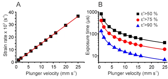
Figure S1: Centre line strain rate and corresponding exposure time in relation to plunger

3

velocities of 1-25 mms-1 calculated by CFD. (A) Centre line strain rate varies linearly with 4

plunger velocity. Red line is a straight line fit to the data. (B) Relationship between plunger 5

velocity and the time that a fluid element is exposed to a strain rate () greater than 50 % (

–

75 % (

–

–

(R2 > 0.995 in all cases). 8

10 1

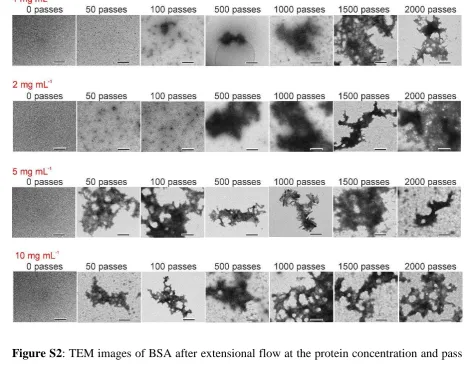
Figure S2: TEM images of BSA after extensional flow at the protein concentration and pass

2

number stated. The plunger velocity in all experiments above was 8 mm s-1 (strain rate = 11750 3

s-1_{, shear rate = 52000 s}-1_{). Images taken at 10000× magnification, scale bar = 500 nm.}

4

11 1

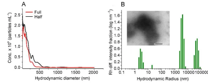
Figure S3: Control experiments under reduced shear by halving the capillary length. (A)

2

Nanoparticle tracking analysis of BSA after 1000 passes through a half-length (black) or full-3

length (red) capillary. (B) Regularization plot of DLS data obtained for BSA after 1000 passes 4

through a half-length capillary. Four distinct peaks were observed from left to right: Rh = 2.9

5

± 0.7 nm, 19.5 ± 1.5 nm, 3.6 ± 0.9 µm and 44.5 ± 11.9 µm. Inset: TEM image of BSA after 6

1000 passes. The image was taken at 10000× magnification, scale bar = 500 nm. In (A) and 7

(B), the BSA concentration was 5 mg mL-1 and the plunger velocity was 8 mm s-1 (strain rate 8

= 11750 s-1 _{and shear rate = 52000 s}-1_{). Half-length capillaries were made by cleaving the}

full-9

length capillaries with a ceramic tile (Sutter Instruments) and finishing the cleaved capillaries 10

in a Bunsen flame to remove sharp edges, before being used in experiments as stated in the 11

12 1

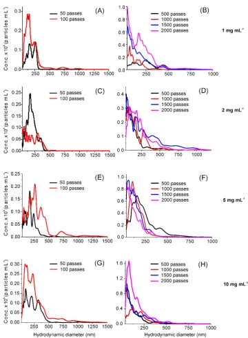
Figure S4: BSA aggregation analyzed by NTA. The experiments were performed at the

2

number of passes indicated at different BSA concentrations. The plunger velocity in all cases 3

was 8 mm s-1 (strain rate = 11750 s-1 and shear rate = 55200 s-1). (A) and (B) at 1 mg mL-1, (C) 4

and (D) at 2 mg mL-1_{, (E) and (F) at 5 mg mL}-1 _{and (G) and (H) at 10 mg mL}-1 _{of BSA. Note:}

5

very few or no aggregates (< 5 particles) were observed for BSA when fewer than 50 passes 6

13 1

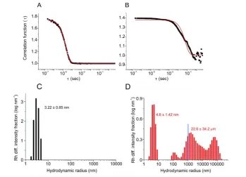
Figure S5: DLS correlation functions (black squares) of (A) native BSA and (B) BSA after

2

2000 passes of extensional flow stress. The BSA concentration in the experiment was 5 mg 3

mL-1, then diluted 1:2 with buffer prior to DLS injection (Supplemental Methods). Fitting a 4

single exponential decay function (red line) to the correlation curve: 5



6

(where A is the amplitude, y0 is a y axis off-set and  is the delay time) yields a good fit for the

7

native sample (monodisperse, R2 = 0.9997) and a poor fit for BSA (disperse, R2 = 0.9719) 8

exposed to extensional flow, indicating the presence of two or more species. Data for poly-9

disperse samples were further analyzed by regularization (C and D) and cumulants analysis 10

(Supplemental Methods). DLS regularization plots showing native BSA (C) and BSA after 11

2000 passes (D). Blue line at 1000 nm indicates the measurement limitation of the technique. 12

In (A)-(D), the BSA solutions were passed through the extensional flow device at a plunger 13

velocity of 8 mm s-1 (strain rate = 11750 s-1 and shear rate = 52000 s-1). 14

14 1

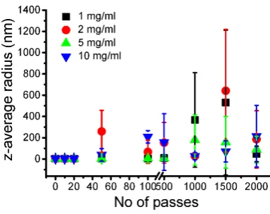
Figure S6: Plot of the z-average radii of 1, 2, 5 and 10 mg mL-1 BSA as a function of pass 2

number, obtained by cumulants analysis of the DLS data (Supplemental Methods). The plunger 3

velocity was 8 mm s-1 (strain rate = 11750 s-1 and shear rate = 52000 s-1). Error bars represent 4

the error from two independent experiments except 2 mg/mL 1000 passes (N =1). 5

15 1

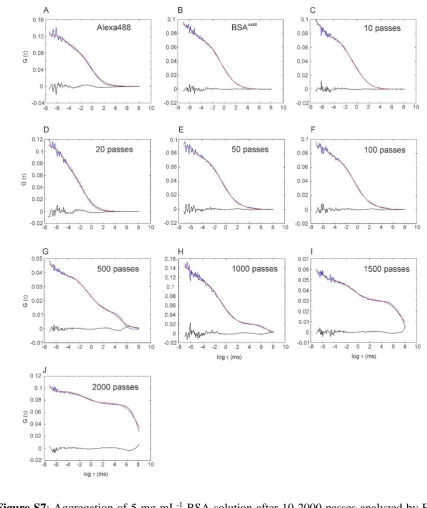
Figure S7: Aggregation of 5 mg mL-1 BSA solution after 10-2000 passes analyzed by FCS. 2

Each plot shows the autocorrelation function (blue lines), their fits to a two component fit (red 3

lines) and residuals (black lines). (A) Alexa-488 dye alone, single diffusion component (B) 4

BSA-Alexa-488 prior to extensional strain, (C) after 10 passes, fitted to a single diffusion 5

component model. Panels (D-J) show a two diffusion component fit of 20, 50, 100, 500, 1000, 6

1500 and 2000 passes, respectively. The plunger velocity was 8 mm s-1 (strain rate = 11750 s-1 7

16 1

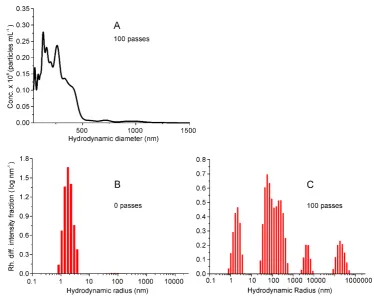
Figure S8: Analysis of extensional flow induced aggregation of 5 mg mL-1 2m by NTA (A)

2

and DLS (B and C). (A) NTA of 5 mg mL-1 2m after 100 passes at a plunger velocity of 8 mm

3

s-1 _{(strain rate = 11750 s}-1_{). Note: no aggregates were visible in the native (0 passes) sample or}

4

following 20 passes. (B) DLS regularization plot of native 2m. The peak shows the mean Rh

5

= 2.5 ± 0.1 nm, a value consistent with that determined using NMR (10). (C) DLS 6

regularization plot of 2m after 100 passes of extensional flow at a plunger velocity of 8 mm s

-7

1 _{(strain rate = 11750 s}-1_{). Four distinct peaks were observed from left to right: R}

h = 2.0 ± 0.3,

8

148 ± 13, 4761 ± 125 and 207662 ± 2261 nm. Cumulants analysis of the DLS data obtained 9

PDI values of 0.21, 0.6 and 0.71 after 0, 20 passes and 100 passes, respectively. 10

17 1

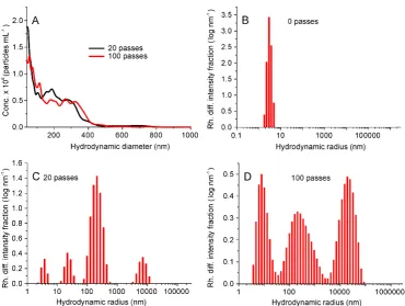
Figure S9: Analysis of extensional flow-induced aggregation of 0.5 mg mL-1 _{GCSF-C3 by}

2

NTA (A) and DLS (B-D). (A) NTA of GCSF-C3 subjected to extensional flow for 20 or 100 3

passes at a plunger velocity of 8 mm s-1 _{(strain rate = 11750 s}-1_{). Note: no particles/aggregates}

4

were observed in the native sample (0 passes). (B) DLS regularization plot of native GCSF-5

C3. A single dominant peak at Rh = 3.5 ± 0.8 nm is observed. (C) DLS regularization plot of

6

GCSF-C3 after 20 passes at the same velocity as in (A). Four distinct peaks were observed 7

from left to right: Rh = 3.7 ± 0.2, 24 ± 3, 218 ± 5, and 7091 ± 19 nm. (D) DLS regularization

8

plot of GCSF-C3 after 100 passes. The three apparent peaks observed were merged due to high 9

sample dispersity precluding resolution into discrete peaks, with the mean Rh = 8750 ± 1400

10

nm. Cumulants analysis of the DLS data yields PDI values of >0.6 for both the 20 and 100 11

passes and < 0.1 for the native sample (0 passes). 12

18 1

Figure S10: Analysis of extensional flow induced aggregation of 0.5 mg mL-1 mAb1 by NTA 2

(A) and DLS (B-D). (A) NTA of mAb1 subjected to extensional flow for 20 or 100 passes at a 3

plunger velocity of 8 mm s-1 (strain rate = 11750 s-1). Note: the native protein (0 passes) did 4

not contain any visible particles/aggregates. (B) DLS regularization plot of native mAb1. A 5

single dominant peak at Rh = 4.8 ± 1.1 nm is observed. (C) DLS regularization plot of mAb1

6

after 20 passes of extensional flow at the plunger velocity indicated in (A). Four peaks were 7

observed form left to right: Rh = 3.9 ± 0.7 nm, 76 ± 11 nm, 4.3 ± 2.5 µm and 117.4 ± 37.1 µm.

8

(D) DLS regularization plot of mAb1 after 100 passes of extensional flow at the plunger 9

velocity indicated in (A). The 1st _{peak (left) observed had a mean R}

h = 8.1 ± 4.1 nm, whilst the

10

2nd and 3rd peaks (right) were merged due to high sample dispersity precluding resolution into 11

discrete peaks (mean Rh = 20.3 ± 1.0 µm). Cumulants analysis of the DLS data yields a PDI

12

19 1

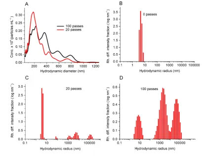
Figure S11: Analysis of extensional flow-induced aggregation of 0.5 mg mL-1

2

MEDI1912_WFL by NTA (A) and DLS (B-D). (A) NTA of MEDI1912_WFL subjected to 3

extensional flow for 20 or 100 passes at a plunger velocity of 8 mm s-1 (strain rate = 11750 s -4

1_{). Note: no particles/aggregates were visible in the native sample (0 passes). (B) DLS}

5

regularization plot for native MEDI1912_WFL. A single peak is observed, with Rh = 6.61 ±

6

3.04 nm. (C) DLS regularization plot for MEDI1912_WFL for 20 passes at the plunger velocity 7

indicated in (A). Three peaks are observed form left to right: Rh = 7.05 ± 2.2 nm, 117.5 ± 44.9

8

nm and 212 ± 93.5 µm. (D) DLS regularization plot for MEDI1912_WFL for after 100 passes 9

at the plunger velocity indicated in (A). Three peaks were observed from left to right: Rh = 2.72

10

± 0.5 nm, 281 ± 63.5 nm and 34.1 ± 10.6 µm. Cumulants analysis of the DLS data yields PDI 11

values of 0.3 for the native sample (0 passes) and > 0.6 for both the 20 and 100 passes samples. 12

20 1

Figure S12 Analysis of extensional flow-induced aggregation of 0.5 mg mL-1 MEDI1912_STT 2

by NTA (A) and DLS (B-D). (A) NTA of MEDI1912_STT subjected to extensional flow for 3

100 passes at a plunger velocity of 8 mm s-1 _{(strain rate = 11750 s}-1_{). Note: no}

4

particles/aggregates were detected in the native sample (0 passes). (B) DLS regularization plot 5

for native MEDI1912_STT. A single peak is observed, with Rh = 5.2 ± 1.6 nm (C) DLS

6

regularization plot MEDI1912_ STT after 20 passes at the plunger velocity indicated in (A). 7

Three peaks are observed, with Rh = 4.1 ± 0.6 nm, 3.0 ± 0.8 µm and 57.4 ± 23.9 µm (D) DLS

8

regularization plot for MEDI1912_ STT after 100 passes. The 1st _{peak observed (left) had a}

9

mean Rh = 11.49 ± 2.42 nm, whilst the 2nd and 3rd peaks (right) were merged due to high sample

10

dispersity precluding resolution into discrete peaks (mean Rh = 17.84 ± 22.24 µm). Cumulants

21

analysis of the DLS data yield PDI values of 0.1, 0.3 and > 0.6, for the 0, 20 and 100 passes 1

samples, respectively. (E) TEM image of native MEDI1912_STT. (F) TEM image of 2

MEDI1912_STT after 100 passes at the velocity indicated in (A). The images in (E) and (F) 3

were obtained at 10000× magnification. Scale bar = 500 nm. 4

22 1

Figure S13: Analysis of stressed BSA incubated with IAEDANS dye ex situ. Top image

2

shows the gel excited by UV light provided by a UV-trans illuminator. Bottom image is the 3

same gel stained with Coomassie Brilliant Blue. A 5 mg mL-1 BSA solution was stressed for 0 4

– 100 passes in the presence or absence of 0.5 mM TCEP at a plunger velocity of 8 mm s-1 5

(strain rate = 11750 s-1). The IAEDANS was added after a relaxation period. 6

7

8

9

10

11

12

13

14

23 1

Figure S14: Percentage of insoluble BSA after extensional flow in the presence or absence

2

of reductant. Percentage of insoluble material following extensional flow stress of 5 mg mL-1

3

BSA for 100 passes at plunger velocities of 8 or 14 mm s-1 _{(strain rates = 11750 and 20481 s}

-4

1, respectively) in the absence (-TCEP) or presence (+ TCEP) of 0.5 mM TCEP. Error bars 5

represent the error from two independent experiments. 6

7

8

9

10

11

12

13

14

24

Table S1: Values associated with the experimental flow field. These values are assumed

1

constant unless otherwise stated. 2

Entity Value

Syringe diameter 4.61 mm Capillary diameter 0.3 mm Plunger velocity 8 mm s-1 Velocity in capillary 1.9 m s-1 Volumetric flow rate 0.13 mL s-1 Reynolds number (syringe) 37

Reynolds number (capillary) 570 Centre line strain rate 11750 s-1 Centre line shear rate 52000 s-1 3

4

5

6

7

8

9

10

11

12

13

25

Table S2: The number of peaks and their corresponding mean hydrodynamic radii (nm)

1

obtained by regularization analysis of DLS data for 1, 2, 5 and 10 mg mL-1 _{BSA subjected to}

2

extensional flow. The protein solutions were at a plunger velocity of 8 mm s-1 (strain rate = 3

11750 s-1 and shear rate = 52000 s-1). Particles larger than 5 m are outside the accurate limits 4

of size determination for DLS, but are shown for completeness (4). 5

Protein Conc.

No. of passes

Peak 1 (nm)

Peak 2 (nm) Peak 3 (nm) Peak 4 (nm)

1 mg mL-1 _{0 3.4 ± 0.9}

10 3.1±0.6 1748±434

20 3.3±0.9

50 3.2±0.8 5955±2106

100 3.5±1.2 310±80

500 3.3±0.66 77±25 994±357

1000 7.0±5.7 1422511450

1500 5.2±24 16490±16460

2000 3.0± 0.5 139± 20 1915± 576 140564

± 172260

2 mg mL-1 _{0 3.3±1}

10 3.2±0.7

20 3.2±0.8

50 2.9±0.8 857±812 367715±237351

100 2.2±0.6 98±32 693±227 16215

±5780

500 4.1±1.1 887±705 26911±12802

N =1 1000 11.2±3.8 58522±129872

1500 4.4± 2.2 24678±29920

2000 8.4±1.6 1230±571 27912±12189

5 mg mL-1 _{0 3.2±0.8}

10 3.4±1.0 506±157

20 3.3±0.8 292±76

50 3.1±0.6 2146±700 52739±24392

100 2.5±0.9 36±9 31158±7720

500 3.2±1 352±100 37600±8400

1000 4.6±1.4 22636±34198

1500 4.2±2.6 13983±20580

2000 3.7±0.8 82±21 26683±39806

10 mg mL-1 _{0 3.3±1.0}

10 3.3±0.9

20 2.7±0.3 15598±4812

50 2.4±0.3 520±140 3713±1268

100 2.9±1.1 5877±12817

500 3.5±0.9 65±9 12383±12494

1000 2.8±0.5 26±5 2896±2044 65301

±23533

1500 3.7±1.7 531±441 12722±5140

26

Table S3: The polydispersity index (PDI) of 1, 2, 5 and 10 mg mL-1 BSA after 0-2000 passes 1

at a plunger velocity of 8 mm s-1 _{(strain rate = 11750 s}-1 _{and shear rate = 52000 s}-1_{). PDIs were}

2

calculated from the z-average radii and distribution widths shown in Figure S6. 3

PDI z-average radius (nm)

PDI z-average radius (nm)

PDI

z-average radius (nm)

PDI z-average radius (nm) Number

of passes

1 mg mL-1 _{2 mg mL}-1 _{5 mg mL}-1 _{10 mg mL}-1

0 0.16 3.6 0.14 3.5 0.13 3.5 0.13 3.5

10 0.22 3.5 0.09 3.5 0.26 3.6 0.19 3.4

20 0.16 3.5 0.12 3.5 0.25 3.5 0.23 3.4

50 0.27 3.5 0.58 259.2 0.34 4.0 2.19 39.6

100 0.3 3.6 2.66 66.7 0.39 4.4 0.08 208.4

500 1.49 9.4 1.56 153.2 0.88 5.2 2.84 158.4

1000 1.47 366.7 0.71 26.6 1.75 177.4 1.55 26.7

1500 1.65 530.1 0.81 641.6 2.42 156.5 1.94 71.9

2000 2.39 47.4 2.11 185.3 2.0 87.9 1.83 214.4

4

27

Table S4: Hydrodynamic radii obtained by fitting the FCS data shown in Figure S7.

1

2

3

4

5

6

7

8

9

No. of passes Mean Rh (nm)

1 mg mL-1 _{2 mg mL}-1 _{5 mg mL}-1 _{10 mg mL}-1

BSA 5.0 5.2 2.7 4.2

10 16.5 16.4 8.8 7.3

20 27.6 15.6 23.3 21.3

50 40.6 47.5 34.9 146.7

100 53.7 98.7 52.0 223.3

500 101.3 17.5 256.8 17.2

1000 1280.2 1029.7 3089.4 1024.2

1500 1204.0 12492.8 3403.0 2921.8

28

Table S5: Summary of protein characteristics.

1

BSA mAbs GCSF-C3 2m

Amino acids 583 ~1400 175 100

MW (kDa) 66 148 18.8 11.86

Size (nm) 3.5 6 2.5 2.3

pI (25 °C) 4.7

mAb1 9.42 WFL 8.64

STT 8.64

5.65 6.05

Structure

PDB Code:

3V03 1HZH 1RHG 2XKS

280 (M-1 cm-1) 43824

mAb 1 = 207360 WFL = 239440

STT = 228440

10220 20065

2

3

4

5

6

7

8

9

10

11

12

13

14

15

29

References

1

1. Yadav S, Shire SJ, & Kalonia DS (2011) Viscosity analysis of high concentration bovine serum 2

albumin aqueous solutions. Pharm. Res. 28(8):1973-1983. 3

2. Aris R (2012) Vectors, Tensors and the Basic Equations of Fluid Mechanics (Courier 4

Corporation). 5

3. Jaspe J & Hagen SJ (2006) Do protein molecules unfold in a simple shear flow? Biophys. J.

6

91(9):3415-3424. 7

4. Hassan PA, Rana S, & Verma G (2015) Making Sense of Brownian Motion: Colloid 8

Characterization by Dynamic Light Scattering. Langmuir 31(1):3-12. 9

5. Hanlon AD, Larkin MI, & Reddick RM (2010) Free-solution, label-free protein-protein 10

interactions characterized by dynamic light scattering. Biophys. J. 98(2):297-304. 11

6. Roger V, Cottet H, & Cipelletti L (2016) A New Robust Estimator of Polydispersity from 12

Dynamic Light Scattering Data. Anal. Chem. 88(5):2630-2636. 13

7. Gell C, et al. (2008) Single-molecule fluorescence resonance energy transfer assays reveal 14

heterogeneous folding ensembles in a simple RNA stem-loop. J. Mol. Biol. 384(1):264-278. 15

8. Tipping KW, et al. (2015) pH-induced molecular shedding drives the formation of amyloid 16

fibril-derived oligomers. Proc. Natl. Acad. Sci. USA 112(18):5691-5696. 17

9. Gell C, Brockwell D, & Smith A (2006) Handbook of Single Molecule Fluorescence

18

Spectroscopy (Oxford University Press, Oxford). 19

10. Mukaiyama A, et al. (2013) Native-S H -Microglobulin as Revealed by 20

Kinetic Folding and Real-Time NMR Experiments. Journal of Molecular Biology 425(2):257-21

272. 22