Predicting response from load : an application of multivariate analysis techniques to computer performance data

PREDICTING RESPONSE FROM LOAD: An application of multivariate analysis techniques to computer performance data.

Presented in part fulfillment of the requirements for the degree of Master of Science in Statistics

by

Christopher Eric Stevenson

The work reported on in this thesis is

entirely that of the author except where otherwise noted and attributed.

C.

C.E. Stevenson

Ho-Vv

C O N T E N T S

SUMMARY 1

PREFACE 3

CHAPTER ONE - INTRODUCTION 4

1.1 Analysing Computer Performance Data 4 1.2 Problems Associated with Tuning a

Computer 5

1.3 The Data Available for Analysis 8

CHAPTER TWO - AN INDEX OF LOAD 12

2.1 Principal Component Analysis 12 2.2 Calculating the Index of Load 13 2.3 Assessing the Index of Load 14 CHAPTER THREE - FITTING THE REGRESSION EQUATIONS 23

3.1 Removing the Effect of Load 23

3.2 Fitting the Equations 26

3.3 Further Combining the Groups 28 3.4 Examining the Predictive Power of the

Equations 47

CHAPTER FOUR - ASSESSING THE EFFECT OF A CHANGE

IN THE PARAMETERS 57

4.1 Assessing the Change in Response 57 4.2 The Test Procedure in Practice 58

CHAPTER FIVE - CONCLUDING REMARKS 64

BIBLIOGRAPHY 66

-ooOoo-1.

SUMMARY

This thesis takes the form of a case-study. It is concerned with the application of principal component analysis and regression analysis to computer performance data.

The problem considered was that of finding a way to quantitatively assess the effect of changes in a

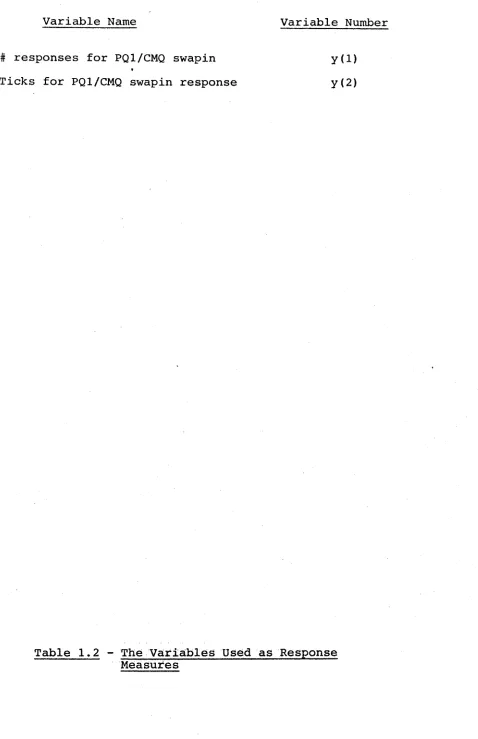
computer's scheduling parameters on its response. Two variables (# responses for PQI/CMQ swapin, denoted by y(l), and ticks for PQI/CMQ swapin response, denoted by y(2)) were taken as measures of response and a procedure devised to assess, for a given load, the change in these variables brought about by a change in the parameters.

In order to make such an assessment, a single

measure of load is required. There are 26 different measures of the load on different parts of the system and these

measurements are recorded automatically every minute that the system is operating. The data available for this study was all these measurements for the months April, May and June 1980. A subset of 1000 points was taken from the April and May data and a principal component analysis done on this subset. Some properties of the first principal

component were studied and this component was accepted as an index of load.

2.

error it was found that an equation for the transformed variable Z = log(y(2)) could be found for most but not all of the groups. Then it was found that the groups could be further combined without significant loss of information into three groups and that equations could be fitted for y (1) to all three groups but for Z only to two of the

groups. The ability of these equations to predict response from load was then tested by drawing a sample of points from the June data and comparing the observed values of y (1) and Z with the values predicted by the equations.

Thus the procedure to assess the effect of a parameter change was to select a sample of points from

immediately after such a change and use the equations (which have been estimated using data from before the change) to predict the response variables. These predictions represent estimates of the expected response for these points under the old parameter settings and the observed values represent the actual response under the new settings. Thus a

comparison between the observed and the actual response gives a measure of the change in response brought about by the parameter change.

3. PREFACE

This case study is an attempt to provide a solution to problems being experienced by users of the DEC-10 computer in the Coombs building in the A.N.U. The main problem is to find a way of setting the computer's

scheduling parameters so that the machine operates in the most efficient manner. This is currently done largely by

trial and error. A prerequisite for finding such an

'optimal' solution is a method of quantitatively assessing the effect of changes in the parameters on the operation of the computer, and it is this aspect of the problem that I was asked to study. Once this question has been answered, there remains the question of the best way of using such a quantitative method to find the optimal parameter setting. However, this question involves a more detailed investigation of the computer system and is beyond the scope of this study.

In seeking to find a quantitative assessment of the effect of parameter change, I have used a number of variables as measures of load and response. The use of these variables raises the question of their suitability as measures of load and response. However, a detailed

consideration of whether these were the most suitable

4.

CHAPTER ONE - INTRODUCTION

1.1 Analysing Computer Performance Data :

The usual approach to the analysis of computer performance data is to develop a model of the computer

system based on queueing theory. The programs being run on the computer are represented as waiting in a collection of queues to be 'served' by the various parts of the computer system (for example, disk or tape input/output units) and the whole computer is represented as a system of queues with the programs moving from one queue to another until all

their requests for the machine's resources are satisfied. Unfortunately this approach has two main disadvantages.

First of all, such models are usually very

complex (because of the complex nature of the system they are required to model). This means that they are very

expensive in terms of the time required to develop them and require a high level of mathematical and statistical

sophistication. These are resources that many computer installations (and in particular the computer installation which is the subject of this case study) do not have readily available.

The second problem is that in order to make

such models mathematically tractable, a number of simplifying assumptions are required and these assumptions are often

questionable for real systems. Consequently the results from the applications of these models are not sufficient to

5.

for example Grenander and Tsao (1972))

For these reasons, I have not attempted this sort of modelling. Instead, I have tried to develop equations which describe the behaviour of the system

without trying to model in detail the nature of the system. I have treated the system as an unknown 'black box’ and I have used regression analysis to estimate equations which relate the inputs of this system to its outputs. This approach avoids the complexity of detailed modelling and still should provide an adequate solution to the particular problem with which this case study is concerned. This sort of approach (the application of techniques such as regression analysis to specific problems in the analysis of computer performance data) was suggested by Grenander and Tsao

(Grenander and Tsao (1972)).

1.2 Problems Associated with Tuning a Computer :

For the purposes of this discussion, the computer can be represented diagrammatically in the following way:

LOAD

•> RESPONSE

SCHEDULING PARAMETERS

Here we have a number of demands for the use of the machine's resources (the load) and a number of parameters governing

6.

control is the set of scheduling parameters and these must be set so that the system operates in the 'most efficient' manner. This process is known as 'tuning' the computer. For the purpose of this case study, an 'efficient' system is one which has a minimum response time for any given load.

The difficulty with tuning arises from the fact that there is no theoretical way of predicting the effect that these parameters have on the system. They must be set by trial and error. Furthermore, once they have been set, there is no immediate way of assessing their effect. Thus an essential prerequisite for successful tuning is a method of quantitatively assessing the effect of a change in the parameters. The aim of my case study is to find such a method.

One obvious way of solving this problem is to combine the scheduling parameters and the measures of load into one equation with parameters estimated to give a

prediction of response time. This would give a direct measure of the effect of each parameter on the response. The difficulty with this is that there are twenty-one

different scheduling parameters and they have been changed only a few times, so that there is insufficient data available to estimate such an equation. Furthermore it is not practical to vary each of these parameters often enough to generate

such data, since this would interfere with the normal operation of the computer.

7.

parameters can then be changed and the response measured. The predicted response can be calculated from the equations and this will provide a measure of what the response

would have been under the old scheduling parameters. This can be compared with the observed response (which is a measure of what the response is under the new scheduling parameters) and the comparison will provide a measure of the effect of the change in parameters. In this way,

several changes of the parameters can be made and the effect of each assessed, relative to the base period. The setting of the parameters which gives the greatest decrease in

response time can then be adopted as the new system parameter values.

There is, however, a problem with this approach. The relationship between the load and the response is

likely to vary with the load. An equation which gives good results when the load is high, that is, when there are many competing requests for the machine's resources and the

system has difficulty responding to these requests, is unlikely to give good results for low load, when there are

few demands for these resources and the system has little difficulty in meeting these demands. One way of overcoming this problem is to calculate different equations for

different levels of load. However there is not one overall measure of load. Instead there are twenty-six

different measures of load on different parts of the system. Therefore the first step in the analysis must be to find a way of combining these twenty-six variables into one overall measure of load.

8.

the derivation of such a measure or 'index' of load. In chapter three I have described the use of this index to identify periods of high, medium and low level load in order to calculate separate prediction equations for each period, thus overcoming the problem of the varying relation­ ship between load and response. Chapter four then describes the use of these equations to assess the effect of the

change in parameters.

1.3 The Data Available for Analysis :

The data used for this study is collected automatically by the system every minute while it is

running. The analysis was done on data for April and May 1980, and the accuracy of the estimated prediction equations was checked by predicting response for June 1980 and then comparing it with the observed response for that month.

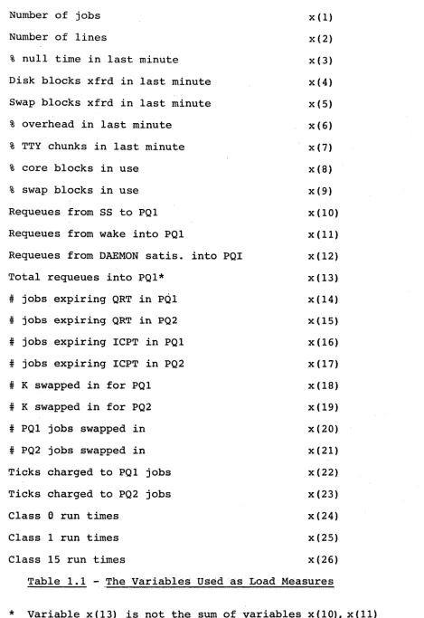
The variables used as measures of load are listed in Table 1.1. These are variables which can be used as

measures of load on various parts of the system. For the sake of brevity, I have also given each load variable a number and throughout this analysis I shall refer to them as x (j), where j is the variable number.

The question of what constitutes a good measure of response is an unresolved one and a discussion of it

9.

this response time but there are two variables which can be used as a measure of the number of jobs which have had requests satisfied in a given time (in this case in the previous minute). Therefore a rise in one or both of

Variable Name _{Variable Number}

Number of jobs x(l)

Number of lines x(2)

% null time in last minute x(3)

Disk blocks xfrd in last minute x(4) Swap blocks xfrd in last minute x(5)

% overhead in last minute x(6)

% TTY chunks in last minute x(7)

% core blocks in use x(8)

% swap blocks in use x(9)

Requeues from SS to PQ1 x(10)

Requeues from wake into PQ1 x(ll)

Requeues from DAEMON satis, into PQI x(12)

Total requeues into PQI* x(13)

# jobs expiring QRT in PQI x(14)

# jobs expiring QRT in PQ2 x(15)

# jobs expiring ICPT in PQI x(16)

# jobs expiring ICPT in PQ2 x(17)

# K swapped in for PQI x(18)

# K swapped in for PQ2 x(19)

# PQI jobs swapped in x(20)

# PQ2 jobs swapped in x(21)

Ticks charged to PQI jobs x(22)

Ticks charged to PQ2 jobs x(23)

Class 0 run times x(24)

Class 1 run times x(25)

Class 15 run times x(26)

Table 1.1 - The Variables Used as Load Measures

Variable Name Variable Number

# responses for PQ1/CMQ swapin y (1) Ticks for PQ1/CMQ swapin response y(2)

1 2.

CHAPTER TWO - AN INDEX OF LOAD

2.1 Principal Component Analysis :

When a principal component analysis is done on an m - dimensional data set, the components with the n highest eigenvalues represent the axes of the 'best fitting'

n - dimensional subspace of the original m - dimensional space. In other words, if the points in the m - space are projected orthogonally onto an n - space, the sum of squares of the distances between the points and their projections is minimised by taking as the axes of the n - space, the n principal components with the highest eigenvalues. This was in fact the way that the principal component analysis technique was first used by Pearson in 1901 and later by Frisch in 1929 (see for example Rao (1965)). Therefore, the

first principal component (i.e. the one with the highest eigenvalue) is the best fitting line, in the least squares sense, to an m - dimensional data set.

The variables under consideration in this case study (that is, the variables x(l) to x(26)) are all, to some extent, measures of the load on different parts of the system. Therefore, it seems reasonable to assume that the first principal component of the data (i.e. the line of closest fit, or the linear combination of the variables which explains the highest percentage of the variation)

represents a load 'factor' or overall measure of load. This follows the approach suggested, in a different context, by Kendall, who said;

In the behavioural sciences, especially in economics, we are frequently compelled to

1 3.

p-dimensional system, so to speak, into one dimension. Familiar examples are index- numbers of prices, money wage rates, cost of living, business activity, and so forth. Such index-numbers are usually constructed by

weighting the constituent items by quantities which, in some sense, reflect their relative

importance. We may, however, approach the subject from the point of view of principal components and ask : if the variation is to be summarised as nearly as possible in a

linear combination of the variables, which is the best linear function? From this angle the first principal component, which is an answer to the question, furnishes its own weights.

(Kendall (1975))

I have therefore done a principal component analysis of the data and used the first component as an 'index of load'.

2.2 Calculating the Index of Load :

The principal component analysis was done on the data for April and May. Since the data was collected every minute for each day of those months, this means that there should be 1440 points for each day, giving a total of 87840 points. In fact there are not quite this many, since for part of that time the computer was not functioning

because of machine breakdowns, so that there are only 80899 measurements of each of the variables for this two month period. Obviously this is still too much data to operate on directly, since any calculations would take a lot of computer time and be subject to a large rounding error. Therefore I have selected instead a random sample of 1000 points (500 from April and 500 from May) and

based the calculation of the index on these.

1 4.

m e a s u r e m e n t (for example, some are counts of the number of

jobs wa i t i n g in particular job queues in the system, while others me a s u r e such things as units of core storage u s e d ) . Furthermore, even where two variables are the same type of measurement, they often have quite d i f f erent standard

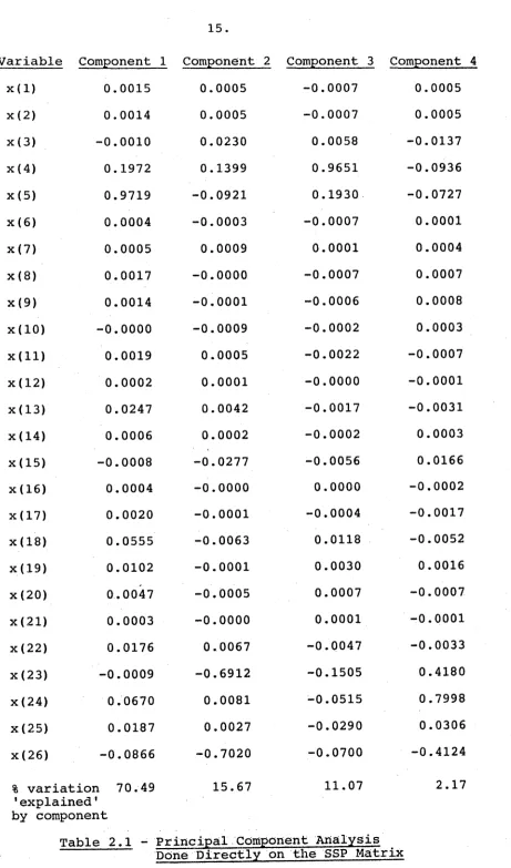
deviations. The effect of this can be seen in the results of an analysis done dire c t l y on the sums of squares and products (SSP) m a trix (Table 2.1) where the analysis ap p a r e n t l y identified only two variables as contributing s ignificantly to the index (variables x(4) and x(5)).

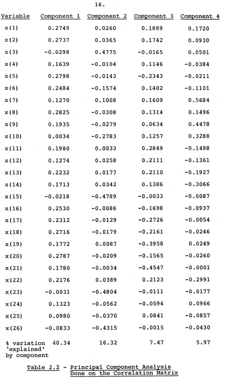
To overcome this problem, I have used the corre l a t i o n mat r i x e s t i mated from this SSP matrix. The results of the analysis done on the variables in this standardised form are given in Table 2.2.

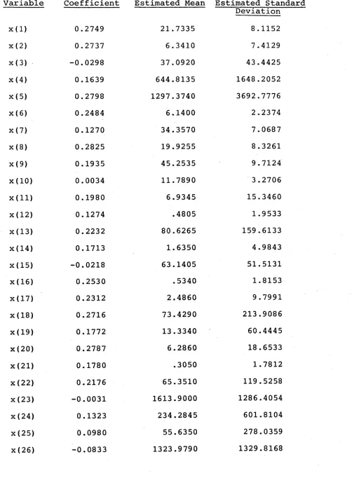
Thus the final.form of the index is:

I = 1 26 a 1 (*( j) - x( j) )

j — i a •

where

a j

are the e s t i mated component coefficients, and

i j 26 are the estimated means, and *(j) \

J j = i

q I are the estimated

3 1 J -l —. 1

the twenty-six load variables, in T a ble 2.3.

2.3 A s s e s s i n g the Index of Load

standard deviations of

These estimates are given

The question now arises : can we attribute any

1 5.

Variable Component 1 Component 2 Component 3 Component 4

x {1) 0.0015 0.0005 -0.0007 0.0005

x (2) 0.0014 0.0005 -0.0007 0.0005

x (3) -0.0010 0.0230 0.0058 -0.0137

x (4) 0.1972 0.1399 0.9651 -0.0936

x (5) 0.9719 -0.0921 0.1930 -0.0727

x (6) 0.0004 -0.0003 -0.0007 0.0001

x (7) 0.0005 0.0009 0.0001 0.0004

x (8) 0.0017 -0.0000 -0.0007 0.0007

x (9) 0.0014 -0.0001 -0.0006 0.0008

x (10) -0.0000 -0.0009 -0.0002 0.0003

x(ll) 0.0019 0.0005 -0.0022 -0.0007

x (12) 0.0002 0.0001 -0.0000 -0.0001

x (13) 0.0247 0.0042 -0.0017 -0.0031

x (14) 0.0006 0.0002 -0.0002 0.0003

x (15) -0.0008 -0.0277 -0.0056 0.0166

x (16) 0.0004 -0.0000 0.0000 -0.0002

x (17) 0.0020 -0.0001 -0.0004 -0.0017

x (18) 0.0555 -0.0063 0.0118 -0.0052

x (19) 0.0102 -0.0001 0.0030 0.0016

x (20) 0.0047 -0.0005 0.0007 -0.0007

x (21) 0.0003 - 0.0000 0.0001 -0.0001

x (22) 0.0176 0.0067 -0.0047 -0.0033

x (23) -0.0009 -0.6912 -0.1505 0.4180

x (2 4) 0.0670 0.0081 -0.0515 0.7998

x (2 5) 0.0187 0.0027 -0.0290 0.0306

x (2 6) -0.0866 -0.7020 -0.0700 -0.4124

% variation 70.49 15.67 11.07 2.17

1 explained' by component

Table 2.1 - Principal Component Analysis Done Directly on the SSP Matrix

1 6.

Variable Component 1 Component 2 Component 3 Component 4

x(l) 0.2749 0.0260 0.1889 0.1720

x(2) 0.2737 0.0365 0.1742 0.0930

x (3) -0.0298 0.4775 -0.0165 0.0501

x (4) 0.1639 -0.0104 0.1146 -0.0384

x (5) 0.2798 -0.0143 -0.2343 -0.0211

x (6) 0.2484 -0.1574 0.1402 -0.1101

x (7) 0.1270 0.1008 0.1609 0.5684

x (8) 0.2825 -0.0308 0.1314 0.1496

x (9) 0.1935 -0.0279 0.0634 0.4478

x (10) 0.0034 -0.2783 0.1257 0.3288

x(ll) 0.1980 0.0033 0.2849 -0.1498

x (12) 0.1274 0.0258 0.2111 -0.1361

x (13) 0.2232 0.0177 0.2110 -0.1927

x (14) 0.1713 0.0342 0.1386 -0.3066

x (15) -0.0218 -0.4789 -0.0033 -0.0087

x (16) 0.2530 -0.0086 -0.1698 -0.0937

x (17) 0.2312 -0.0129 -0.2726 -0.0054

x (18) 0.2716 -0.0179 -0.2161 -0.0246

x (19) 0.1772 0.0087 -0.3958 0.0249

x (20) 0.2787 -0.0209 -0.1565 -0.0260

x (21) 0.1780 -0.0034 -0.4547 -0.0001

x (22) 0.2176 0.0389 0.2123 -0.2991

x (23) -0.0031 -0.4804 -0.0111 -0.0177

x (24) 0.1323 -0.0562 -0.0594 0.0966

x (25) 0.0980 -0.0370 0.0841 -0.0857

x (26) -0.0833 -0.4315 -0.0015 -0.0430

% variation 40.34 16.32 7.47 5.97

' explained' by component

Table 2.2 - Principal Component Analysis Done on the Correlation Matrix

I have only shown the first four components. Each of

1 7.

Variable Coefficient Estimated Mean Estimated Standard Deviation

x (1) 0.2749 21.7335 8.1152

x (2) 0.2737 6.3410 7.4129

x {3) -0.0298 37.0920 43.4425

x (4) 0.1639 644.8135 1648.2052

x (5) 0.2798 1297.3740 3692.7776

x (6) 0.2484 6.1400 2.2374

x (7) 0.1270 34.3570 7.0687

x (8) 0.2825 19.9255 8.3261

x (9) 0.1935 45.2535 9.7124

x (10) 0.0034 11.7890 3.2706

x(ll) 0.1980 6.9345 15.3460

x (12) 0.1274 .4805 1.9533

x (13) 0.2232 80.6265 159.6133

x (14) 0.1713 1.6350 4.9843

x (15) -0.0218 63.1405 51.5131

x (16) 0.2530 .5340 1.8153

x (17) 0.2312 2.4860 9.7991

x (18) 0.2716 73.4290 213.9086

x (19) 0.1772 13.3340 60.4445

x (20) 0.2787 6.2860 18.6533

x (21) 0.1780 .3050 1.7812

x (22) 0.2176 65.3510 119.5258

x (23) -0.0031 1613.9000 1286.4054

x (24) 0.1323 234.2845 601.8104

x (25) 0.0980 55.6350 278.0359

x (26) -0.0833 1323.9790 1329.8168

line 2

line 3

- change n to !JIf'...u ~ change n...all).M to , .all

and

18 .

independent measure of load against which this index can be tested (if such a K 1x measure existed, it would not

have been necessary to calculate the index at all). However, there are some factors which indicate that our index is at least consistent with the attributes one would expect of a load measure. These are:

1. The coefficients appear to be in the right proportions. Those variables which should be negatively correlated with load such as x(3) - % null in last minute

(which provides a measure of the time during the last minute that the system was idle), have coefficients with opposite signs to those which should be positively

correlated with load. Furthermore, those variables which are known to be highly correlated with the overall load

(such as x(20) - #PQ1 jobs swapped in) have higher

coefficient values than those which are known to be less correlated with the overall load (such as x(26) - class 15 run times).

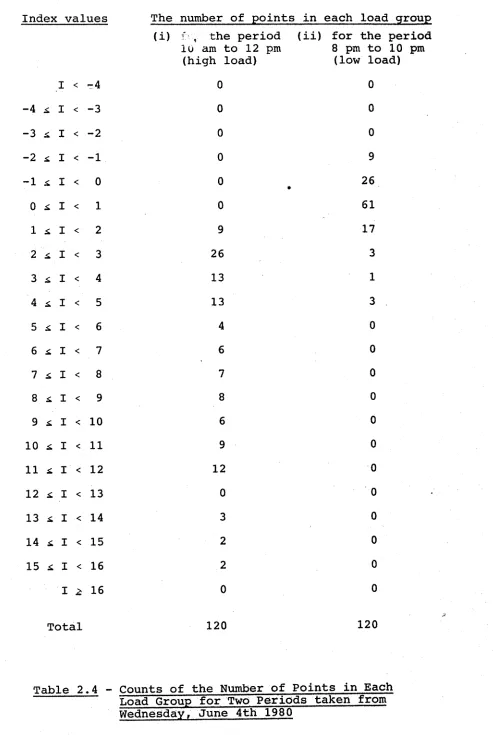
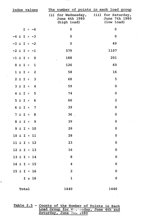
2. The index gives high values for those times of day and days of the week when the system is known to be busy, and low values for times when the system is known to be less busy. This is demonstrated by Tables 2.4 and 2.5. I chose a weekday at random from June 1980 (Wednesday, June 4th) and selected a time when the computer should be busy (10 am to 12 pm) and a time when the computer should not be so busy (8 pm to 10 pm). Table 2.4 gives the counts of the number of points in each load group for each of these periods. Table 2.5 gives a similar comparison between

change iinee V to 16 to road

” I DE 1 against IN’06X2. I f the index truly represents a load factor,

je uould expect that points ide: tifieri as being of high load,

using INDEX2, uould also be identified as being of high load

using INDEX1, and similarly for points of lou load. This appears,

from the graph, to be the case since the plot is roughly linear

1 9.

at the weekend and Table 2.5 confirms this.

3. The index ca± uxated from April and May data agrees closely with that calculated independently from data from June. A sample of 200 points was taken from the June data and the first principal component was estimated

from this. The value of this component for each of the 200 June points was calculated and I called this INDEX 1. Then the value of the index estimated from the April and May data was calculated for each of these points. I called this INDEX 2. Graph 2.1 gives the results of plotting

INDEX 1 against INDEX 2. From this it can be seen that not only are the values of the two indexes similar, but more importantly the ordering of the points is preserved. If our index truly represents a load factor, we would expect that points identified as being of high load, using INDEX 2, would also be identified as being of high load using INDEX 1 and similarly for points of low load. This appears from the graph, to be the case.

These three factors cannot, of course, guarantee that I have correctly identified a load index, though they do lend weight to the use of the component as an index of load. The most important test of the index, however, will be whether or not it can be used to fit a regression

equation to the data. If it can be used for that, it can be regarded as an index of load for the purposes of this study. If not, it is of no use in this study. Thus, the only real way to decide the value of this index is to try to use it in fitting an equation to the data. The

2 0.

Index values The number of points in each load group (i) !* , the period (ii) for the period lo am to 12 pm 8 pm to 10 pm

(high load) (low load)

I < -4 0 0

-4 I < -3 0 0

-3 I < -2 0 0

-2 £ I < -1 0 9

-1 £ I < 0 0 26

•

0 £ I < 1 0 61

1 £ I < 2 9 17

2 I < 3 26 3

3 £ I < 4 13 1

4 I < 5 13 3

5 £ I < 6 4 0

6 £ I < 7 6 0

7 £ I < 8 7 0

8 £ I < 9 8 0

9 £ I < 10 6 0

10 £ I < 11 9 0

11 £ I < 12 12 0

12 £ I < 13 0 0

13 £ I < 14 3 0

14 £ I < 15 2 0

15 £ I < 16 2 0

I 2 16 0 0

Total 120 120

21

Index values The number of points in each load group (i) for Wednesday,

June 4th 1980

(ii) for Saturday, June 7th 1980 (high load) (low load)

I < -4 0 0

-4 < I < -3 0 0

-3 < I < -2 0 49

-2 < I < -1 579 1107

-1 < I < 0 188 201

0 < I < 1 126 60

1 < I < 2 58 16

2 < I < 3 68 5

3 < I < 4 59 0

4 < I < 5 74 0

5 < I < 6 66 2

6 < I < 7 39 0

7 I < 8 36 0

8 < I < 9 39 0

9 < I < 10 26 0

10 < I < 11 28 0

11 < I < 12 23 0

12 < I < 13 16 0

13 < I < 14 8 0

14 < I < 15 4 0

15 < I < 16 2 0

I -a 16 1 0

Total 1440 1440

22

0

1 M O t O O ' T1I-UC 1-1 t J ♦ h

-- s o r X ON ^ •

H ü « «

O C

vC La t « ro H-*-* Cl O CJI I I

o co xr a c j o o u

1 - 0 - 0

—11-r\i

Cl

O

o

■e / » o o a a u u

r-J •*

*

(\) «■

i M W W U • • • --_3-C O ''. GUD c;

HHHl-■fr *

• » #

-1 -P P P

«J» o p- (r u a o t :

«■ •»■

* *

*

r j O O P

i—o —II—o r>m o a

o u t - i a t o >

P I) 'JIT

ÜUÜC

tn tjx W

rjxnors.

C1C.1L1C

H H H M H H H l j H H H l j H H H l

-v^t«i xt

o a -eoc

o a a c

H H H t - H H H 1 - H H m o o

Ü Ü Ü

I I I • I I I I I ♦ • I I I I I I » I ♦ I i 1 I I I I 1 I 4-I I I I I t » I ♦ I I t I I I I I » ♦ I » I I « I I ♦ I I I I I I I I I ♦ I « I t I * I ♦ I I I I » I • I I ♦

insert in line 17

-"The effect of this is to allow the functional form of the equation to be non-linerr,"

end insert after the second p a r a g r a p h

-" The load variables were not standardised by scale and

2 3.

CHAPTER THREE - FITTING THE REGRESSION EQUATIONS

3.1 Removing the Effect of Load :

The reason for calculating an index of load was that since the relationship between response and load is likely to vary with changes in load, the index is needed to identify data with different load levels, and to use this to remove the effect of load from the equation. The way that I have done this is to assume that points of

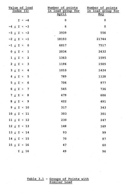
similar load will give rise to the same equation. I have, therefore, divided the data into groups with similar load and fitted an equation to each group. These groups are set out in Table 3.1. This initial grouping was somewhat

arbitrary since I had no prior knowledge of how the

relationship would vary with load. However, the results of the analysis showed that these groups could be combined into even larger groups without significant effect on the equations.

From the table it can be seen that each group contains too much data to operate on directly, so instead I drew a random sample of 200 points from each group (100 points from the April data and 100 points from the May data) and based the estimation of the equations on these subsets. I have described the method used to fit the 'best'

equation in section 3.2 and the results are summarised in Table 3.2.

2 4.

Value of load Number of points Number of points Index (I) in load group for in load group for

April

May-I < -4 0 0

-4 < I < -3 6 0

-3 < I < -2 3939 556

-2 < I < -1 18193 21744

-1 < I < 0 6817 7517

0 < I < 1 2034 2432

1 < I < 2 1363 1595

2 < I < 3 1196 1505

3 < I < 4 1010 1424

4 < I < 5 789 1128

5 < I < 6 706 977

6 < I < 7 545 736

7 < I < 8 479 606

8 < I < 9 422 4SI

9 < I < 10 317 343

10 < I < 11 303 301

11 < I < 12 230 247

12 < I < 13 148 169

13 < I < 14 93 99

14 < I < 15 70 87

15 < I < 16 47 60

I > 16 49 96

2 5.

Value <of load % Variation Explained by "Best" Equation Index (I)

Variable y(l) Variable Z (=log (y(2)))

0 < I < 1 74.6 60.6

1 * I < 2 90.5 63.5

2 * I < 3 89.0 67.7

3 * I < 4 88.4 65.8

4 £ I < 5 90.1 70.5

5 i I < 6 94.7 75.9

6 £ I < 7 96.3 71.5

7 * I < 8 96.7 73.5

8 £ I < 9 95.7 76.0

9 £ I < 10 96.1 56.7

10 * I < 11 97.0 64.7

11 * I < 12 96.5 45.5

12 £ I < 13 97.1 57.7

13 £ I < 14 95.1 30.5

14 £ I < 15 98.1 72.5

15 * I < 16 97.8 84.7

I 16 99.8 96.4

3.2 - % Variation Explained by the 'Best1 Equation in Each of the Load Groups

insert after the first paragraph of section 3.2

-"Data such as this may well exhibit significant multicollinearity, which would affect the stability of the equations. It may have been possible to obviate the effects of this problem by the use of

ridge regression. However, it was- decided not to use this technique for the following reasons, stated in Draper and Smith 1980),

page 324 :

’...use of ridge, regression is perfectly sensible in

circumstances in which it is believed tha* large D-values are unrealistic from a practical point of view, £ However,! in circumstances where.one cannot accept the idea of

r ctrictions on the

(3

! h ° r r j p p r i ori m '•son rest r 5. cr

D 1 1 (or e v e n for assuming that f p ß * s w i 11 n 3 •

I

lues c f tho

take larn9

valuec . Ihcrefore ridge regression was not use;. Inslead it was assumed that, by only using those co-variables which significantly contributed to the equation ie. had significant t-vaiues), the

2 6.

transformation gave the best fit.

The data in Table 3.2 are only given for index values above zero. The reason for this is that only a few of the points with index values below zero have non-zero values for their associated response variables. Thus it is difficult to fit meaningful equations to these points and since, in tuning the computer, the response for

periods of high load is of most interest, it did not seem worthwhile to try.

3.2 Fitting the Equations :

The Genstat system was used to fit the regression equations and the ’best' prediction equation was found by using the Genstat commands for the automatic selection of co-variables (see the Genstat manual volume 1 chapter 7 section 5). There are three such commands in the Genstat system. They are the BEST command, the WORST command and the MINIMISE command. The effect of these is best described with a specific example.

If we have an equation Y = a +bX^ and we have three further possible co-variables X2 • X 3 anc^ X 4 then the

statement

'BEST' X2 ,X3 ,X4

finds the effect of adding to the equation each of X2 , X^ and X4 on its own and then adds to the equation the one that gives the smallest residual mean sqaure (RMS). If no

variable reduces the RMS, then the equation is not changed (i.e. no variable is added).

In a similar way, if we have the equation Y = a + b 1X 1 + b 0X~ + b 0X. -I- b.X.

2 7. ’WORST' X0 ,X,,X.

2 3 4

will find the effect of dropping each of the variables, and if at least one of these operations reduces the RMS, then that variable, whose removal from the equation gives the greatest reduction in RMS, is removed.

The statement

'MINIMISE' X 2 ,X3 ,X4

is in a sense a combination of 'BEST' and 'WORST' in that it will either add or delete a variable in order to achieve the greatest possible reduction in RMS. Again if no reduction is possible the equation remains unchanged.

Therefore the procedure used to fit the equations was as follows:

1. The statement 'BEST' X(l...26)

was used to find the load variable which gave rise to the least RMS in the equation Y = a + bX.

2. The statement

'MINIMISE' X(l...26)

was used. This added further variables to the equation, or removed them from the equation, and it was repeated until no further reduction in RMS was possible.

3. Finally the t-value for each coefficient was examined and if any of them was not significant (at the 95% level) then the variable whose t-value was smallest was removed and the equation re-calculated. This process was repeated until all the variables in the equation had

2 8.

Table 3.2 shows the % variation accounted for by the 'best' equations for each of the load groupings. This is calculated as,

% variation accounted for

= 100 * (total MS - residual MS) / total MS where MS stands for 'mean square', and is different to the usual R2 statistic, which is calculated as above, but with the sum of squares in place of the mean square. The advantage of using this statistic is that it takes into account the number of parameters fitted in the model.

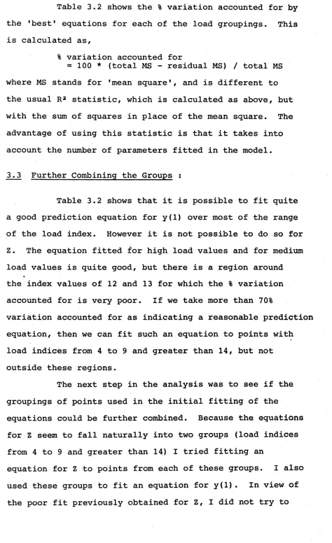
3.3 Further Combining the Groups :

Table 3.2 shows that it is possible to fit quite a good prediction equation for y(l) over most of the range of the load index. However it is not possible to do so for Z. The equation fitted for high load values and for medium load values is quite good, but there is a region around the index values of 12 and 13 for which the % variation accounted for is very poor. If we take more than 70%

variation accounted for as indicating a reasonable prediction equation, then we can fit such an equation to points with load indices from 4 to 9 and greater than 14, but not outside these regions.

The next step in the analysis was to see if the groupings of points used in the initial fitting of the

equations could be further combined. Because the equations for Z seem to fall naturally into two groups (load indices from 4 to 9 and greater than 14) I tried fitting an

replace "These plots do not appear....” (lino 26, page 29) to

”... These are Graphs 3.1 to 3.6” (line 3, page 30) uith -"For the sake of brevity, I have only included the plots for

group 3 (Graphs 3.1 - 3,6). The plots for groups 1 and 2 exhibit substantially the same b eh av io ur ex ce pt that the^e ar«5 no

points which could be classed as outliers.

Graphs s .1 and 3.4 are plots of the fitted values of y l O anH z respectively against the residuals from the equations,

ihe purpose of these graphs is to provide a check for non- homogeneity of variance, and other inadequacies in the model. Goth graphs show evidence of two distinct groups in the data. This in caused by the tendency of points in this gr-up to have either * response of close to zero (or, in the case of Graph 3.4, a rD - noree of - - - ~ f 1 y zero) , or a h i n h rose e n sc , 7 h r- -! i s t ' n r. t

linear pattern in Graph 3.4 comes fr the f 1 that t! :-jr val of the response is zero so that for each point the residual is equal to minus the fitted value. There is some slight evidence of non-homogeneity of variance in Graph 3.1 but this is unlikely to be enoucih to significantly affect the equation. Apart from this and apart from tne evidence of two groups in the data

(which is a characteristic of the data and not of the equation) and apa~t from the anparent outlier (which is discussed below), those plots do not indicate any departure crom the random scatter which would indicate inadequacies in the equations.

Graphs 3.2 and 3.5 are plots of the residuals from the equations for y(l) and z respectively in chronological order. The purpose of these graphs is to show any systematic variation of the residuals with time (eg. do they grow larger or smaller with 1 5 me?) . The residual0 should give the imoression o r p horizontal band constant width. Variations fro this e • 11 e rn m»y indicate (1 ) a non-constant variance (increasing- or decreasing with time) or (?) an extra term in time which should have born included in the model. The graphs do not appear to show any marked departure from the band and thus do not reveal any serious

2 9

.

fit an equation for Z to the points with load indices from 9 to 14. However the equations for y(l) could be fitted to these points and give a good fit, so I fitted an equation for y(l). These groups, which I have denoted groups 1, 2 and 3, are set out in Table 3.3. Although it was possible to fit a reasonable equation for y(l) to

points with load indices below 4, I did not do this because the points of greatest interest in tuning the computer are those of high load.

The 'best' equation was found using the method outlined in section 3.2. I selected a random sample of 200 points from each of the three new load groups (100 points from April and 100 points from May) and used these as a basis for estimating the equations. The results are summarised in Table 3.4. • (In fact group 1 only contains 194 points. This is due to a fault in the computer program which drew the sample. I corrected the fault before

drawing the samples for groups 2 and 3 but it did not seem worthwhile to re-draw group 1, since an equation based on 194 points is not going to be significantly less accurate than one based on 200 points). In addition I plotted graphs of the residuals (1) against the fitted values, (2) in chronological order and (3) re-ordered according to size and plotted against the values of the

expected order statistics from a standard normal distribution (mean zero and variance one). These plots do not appear to show any significant departure from the prediction equation except for group 3. Here the majority of points conform to the expected pattern but there appears to be one

insert after line 3

"Graphs 3.3 and 3.6 are plots of the residuals from the equations for y(l) and z rosnectively, ordered according to size and

plotted against the expected order statistics from a unit normal distribution. If the model is adequate, the residuals should be distributed according to a N(0, O' ) distribution. Thus these plots should be approximately straight lines. This appears to be the case for the graph 3.3 but graph 3.6 has one point uhich lies right off the line. T'his is the same outlier as detected Dy graphs 3.4 and 3.5."

insert after line 16

3 0.

point with a residual value much larger than all the

others. For the sake of brevity, I have only included the graphs for this group. These are Graphs 3.1 to 3.6.

I could not find any unusual factors which might have influenced this value. However, it clearly does not follow the prediction equation and it seemed better to delete this point from the data set and re-estimate the equation. Table 3.5 and Graphs 3.7 to 3.12 summarise the results of this procedure. I have also re-estimated the equation for y(l) from the reduced data set. This may not have been necessary, since the graphs for this equation did not show this point as an outlier, but it seemed

best to remove this point in case there was something unusual about it that the residual graphs did not show. In any case, the equation estimated using 199 instead of 200 points is not likely to be significantly less accurate.

The significance of the difference between the equations based on these further groupings of the data and the original equations can be tested using the Genstat facility for testing grouped data (see the Genstat manual volume 1 chapter 7 section 6). The way that I did this was to take the 'best' equations for each of the combined groups and add to it further terms for the main effects and interactions for a factor which was defined as having a different level for each of the original groups (so that, for example, for group 1, the factor had five levels

3 1.

Group Number Values of Number of points in the

Index I load group

for April for May

1 Vi H V 9 2941 3938

2 9 £ I < 14 1091 1159

3 I i 14 166 243

c h a n g e l i n e 5 t o

-" t ( . 9 9 , 1 9 3 ) £ 2 . 4 * "

a n d l i n e 14 t o -

3 2.

Equation for y(l)

Load variables in Estimate Standard Error t-value equation

x(20) 1.0865 0.0071 152.19

Degrees of freedom for t-value = 193

t( .95,193)* 2.6 * % variation accounted for by equation = 99.2

Equation for Z

Load variables in equation

Estimate Standard Error t-value

constant 4.640311 0.105048 44.17

x (20) 0.053172 0.002684 19.81

x(16) 0.122264 0.022318 5.48

x (12) -0.027735 0.007165 3.87

Degrees of freedom for t-value = 190

t(.95,190)- 2.6 % variation accounted for by equation = 74.5

Table 3.4 part 1 - Equations for Group 1

change line 7 to -”t(.99,l97) d 2.4 change line 18 to —

"t(.99,195) d 2.4 and change line 29 to

*'t (.99,174) d 2.4n

3 3.

E q u a t i o n for y(l)

Load v a r iables in equation

x (20)

x(2)

x(16)

E stimate Standard Error

0.97654

0.25587

0.20771

0.01177

0.04165

0.06420

t-value

82.95

6.14

3.24

Degrees of freedom for t-value = 197

t (.95,197)- 2.6

% v a r i ation a c c o unted for by equation = 99.8

Table 3.4 part 2 - E q u a t i o n for Group 2

Equa t i o n for y(l)

Load variables in equation

Esti m a t e S t a n d a r d Error t-value

constant -9.04290 1.90599 4.74

x (20) 0.96772 0.00994 97.39

x(16) 0.29042 0.04635 6.27

x (1) 0.21452 0.04961 4.32

x (7) 0.15083 0.05443 2.77

Degrees of freedom for t- val u e = 195

t( .95,197)« 2.6

% v a r i ation acc o u n t e d for by e quation = 99 .4

E q u a t i o n for Z

Load variables in equation

E s t i m a t e Stan d a r d Error t-value

constant 6.27683 0.53678 11.69

x (12) -0.02680 0.00128 20.98

x (1) 0.06648 0.01127 5.90

x (4) 0.00009 0.00002 4.45

x(ll) -0.00247 0.00042 5,88

x (21) -0.01953 0.00440 4.44

Degrees of free d o m for t- val u e = 194

t ( . 95 ,194)- 2.6

% var i a t i o n ac c o u n t e d for by equa t i o n = 95.9

add the caption

F IT T E D " V A L U E S V S . R E S ID U A L S ~ V d " ) 34

w r t » c o H v i n ^

I I no I •

r\>cn n

O O C ) O + H

I I I I O' in -p

r- j -r O' rx>

o o o a

l\> D -P Cl m a < 00

> a

r~ .

co +

m

t I I i| I C U M n n a O ^ M

CD CO pr <T\ O O .T><T

Ü Ü D Ü O D O C

I—IHHH

o

* ft

•—• I—I«—M—

INJ

ft

* *

04 -c e i i r i r i ' -peu

prf'-iOOlO' P?MO|C0a'PS Mlo ■» O'-C'M DCO?'PNa'T|'3'

o u o n o a o c G o o q o u n c a a a q n n o c o

h-I HH h

-■p -per

ft

ft «

■»• «■ f t

ft f\J ft ft IV)

ft ft ft

f t f t f v j f t

Mojm

f t f t f t 0 4

ft I ft ft ft ft ! ft

ftf\> ft ft f\> ft ft ft OJ ft ft ft ft M ft ft

* f t * ft

*1

ft ft ft

ft PS ft

ft N» ft

O' o

.J. N'f\. f\J o o a H M M w p i.K j'O '^ -'ö ^ a n

riM I

►“• N I 0 4 I

HHHH HHHH ft ft r\ ft ft ft ft

4

H

HHHHHHHt-HHHH HHHHHHHt-HHHHHHHHHHHt-HHHH

HHHHHHHHHHHHH

p?i\> ci o I I • I I I ♦ I * I I I I I I I ♦ I I I I I I » ♦ I I I I I I I I ■f I I I I I I I ♦ I I I » I « I I ( ♦ » I I I I « I I I

HHt-t *

ard the caption

T u t I K M T t fq y m i m i n s i v n H T S i E

3 5

.

I I

00 00

00 C

C)OC

rvj - c O ' 03

O Ü Ü C

3 ^

m o

o

I I I I - ^c m h j a

h h h h h

I t I I t c w M M n o c i H

• • • • • • • D M -PfTV'TO O0D <7

a o o a u D u c

t-t M M *-1

K)

a I

D I * I

a ♦

*-• » - *-• h - * — * +— * ►— r o P.’ P0 IVj P O

« ' O n w f J M w cf.n O 'cr> -JTD r> •j rij»—• fvj

... . » • • • • • • • ! • • • • • • • • • * •

■prsjr) nocT'-er'Joi'TD rr-to.) 3 •oct> -cKjo c ro

r \ j ' ^ t r x r | i n0' ~ J f n

• • • ' « • • •

o c D d o o o a :.o

P J ft «- ft ft

* *

ft

ft ft

•» * ft * ft ft *

f t *

ft ft *

ft ft ft

* f t

* *

r o

«•

ro

* f t

ft ft * N) ft f M N> N» ft

ft -

ft j r o

f t - »

ft HHWft HH

1

G r a p h 3 * 2

M H H U H - l t - ' M H H M l

H- HHHHMHH

o p c p n o c

►-»h h h

□ C Q C a O Ü C K l C J u

HHH MM MHHHH 4

-I I I • t I I I I ♦ I I I I I I I I I + » I I I I I I I I ♦ « I i t I I I I 4 I I I I I I I I I ♦ I t I I I I I I I 4-I t I I I I I I I ♦ I I I I I I I I 4 I I I • I I I I ♦ I I I » I I I I

H .H M H H H H M H H H H M M H H H *M*M ♦

ad.' the caption

-”The residuals from the equation for y{l) and plotted against the order statistics distribution for the points from group 3

sorted into size order from a unit normal

3 6 . Po Ol UN t> s : x>

r I I I 111

p< * t\> H».r> o r-j

c #

30 1 1

X l\J 1

J» • |

r P t

n + #

a i

m i #

< i

4 - i *

*» t #

—1 i i #

n 4-4 I «

t/N • 1 f\J

O ' 1 #

1 O 4 *■

t I I I I I

OS 00* - 4 O ' U1 P

I •

0 4 o> o ji\j p er» ro o kjp O'lro o r o o

• D O Q D D O O Q C a ' O O U C

r\)

a ♦ n1H H H H H H H H H H H H H H H t—<*-4 »-*4-4 4-4

CD a I a . z o o o 33 IE o mo < • *-ian

J » C 3

—< m </> p a i\) M 04 N)

* 04 04 P 0 4# P in in o

o 4

oo

C ) ♦ t

-oor*j>coHu>mo

MHHf.A rjrv.ro

p p no'-vi oj’» o o k\ jfNj 04 PinU'O' v>r*j•> 1 4— rJ• *4

crjciiwpoo'oop(\>ocno'Poojocr*P(s)r)oi(T' enj n a a ap o o op o a o o a o q t j o u ddoo ci o o o

O ' O ' O' - 4 NP ' J O ' O ' ■» in O ' O ' p *

IT

H H H h - 4-4 4-44-4 4

►-41—t »—I •—I •—I )—I t—

P (\JN> P P 04 P * * 04 M * * r\> * *

H H H 4-4 4— *—4 *“ 4 4—*I—I H H H H ­ H H H H H H 4-4 *-j 4-4 4-4 4-4 H H H H

4-41-4 4

« I » I I I » « 4 » I \ I I I I I I 4 « I I • • I I I » 4 \ \ I I I I I I 4 I I I « I I I I 4 I I I I I I I I « ♦ I I I I J I I I I 4 I » » I I I • I I 4 I I I I I I I I « 4 I I I r I I I I « H »-4 4-4 4

Gra ph 3*3

a d t ■ the c a p tion

T S T T U F S r it b iü ü Ä L S

I I

I pim

►—OC3 c t>cr c o m oo

I I I I t - o a d

O T> O' p

o o o r

3 7

.

I

o r j a d o o M H

• • !•

fsj rj fs) pt o* ca o r\j

c u o d o n a n o

w r ^ c O H i o n ^

■» ro M

*

MMfj rvj rj <\j i\)

• • • > • • •

P <J\ 00 r3;l\J P O' ID

h h h h h h hHh

« • * * ■«■ -* * N ) • f t « '

f \ ) N )

# - O ' M * * N ) O ■» U l U i O I N J *

•«■ * 1> I f t f t NJOJ f f v l W *

f\;Pf\> ft * ■ f r r o r J c ' i O ' O ' c n M

■«■ i.* i - e t \ l f t # ro ftu iro t» ift *

oi +hhhh MhhhHhhhh

-4 uj o. o-Zujp pp c c m / i ' H in y i O'

• • • • • • • • > * • • * • • •

■ o ';» o o p:o'oj ors) p a>.D n

irvnrm n n n r i n r n

O' O' O' I

• • i

N> -P O' ;

a o D c io a o o a o c |u a o o p a u o o n r a p a o

t—<»—11—i;*—Ihh ►m >—I*—*♦—i I—•

H H H U H M t - A - t h -O-1 ♦ I I I I I I I I I

t—i •—t»—-<.—**—<.—*.—< hhhhhhhhh m-t -f

I I I I 1

I I I I I I I I I ■*■ » I I » I I I I I ♦ I • I I I I I t I ♦ I I • I I I I t I * I I I I I I I I « ♦ I I • I I I I 1 I ♦ I I I I I I » I I

cd the caption

K t S l ü U A L b H L U U t U A b A i r . b l f I M t

x i\; e i n e .

3 t *

-n a o

i i i i 3 3 'J O O C* -C D D C 3 C

38

C 3'

rgaw x«!''»: jrv

□onünnoto Hh h h

fl flHHHHHHHt-

fl fl

fl

■fl *

fl fl

fl «j fl fl, fl fl 1

fl fl fl fl ro

*

f l i

fl fl,

fl fl

O + h

#

HHH

mmh'I'J 'vIWr ) f\J

• i • • •

X er 30 CJ M x o% cn

a n a u a a a

H HH ► flt-HtHMfl- 1

NJ

fl fl fl fl

j .

fl fl

f l * !

fl *

fl fl fl

fl *

* f l fl! f l f l * N

3

J

fl

j .

fl fl

N>

f l f l

*

fl fl

ro fl *

*

fl fl i » fl fl fl fl fl

I * r\>

fl fl

f l f l j

f l I f l * * f l

f l *

M

fl fl fl fl

fl

fl *

fl fl

* fl fl fl fl fl fl fl * ro

N *~i I—1 *—* ♦—4 »

.»j ujl»j u j1 <3 x x c x x > n ut| n i ri <> <7S cr> <t> j

• • • • ! • • • • • • • :j N jx <r<rar,rj xi'T' *d ~ jn> xO 'on raK> x cr> ocaonuooDDQDODurnüa t~t >-<*-> t—

»—<»—« *—< t—«»—* t—( » »—t *—<

HHHHI—•«—«•—* »—flHHHHHiH-t ♦

I I I I I I I I » + I I I * I I I I I ♦ I I I 1 I * I I I ♦ I I I • » I I t I ♦ I » I I I I I I ♦ I I • I I I I I I ♦ I I • I • I I I I + I I I « I I I I f l I I I I I I 1 I ♦ • I I 1 I I I I

►-h hHMHHHH fl

T

add the caption

f ? n -s i i y T A i n ~ it fir i> -n \ s a S 1 U nO iS ^ a 39

w r ^ c o H i f l . ' n - o

1 1 M

t-1 1 11 w a o r : 1 • • • • • • CM P N I“) -TOO' 0 • DC o a o c: M

O 4 *~ 1 1

H H H H

1 1 •* • I 1 1 N 1 • I -C 1 0 4 «

1 * 1 1 *■ 1 *• 11 * M 1 * • | ro O' 1 «■ O 4 M 1 M

1 M

1 CM

1 M

1 p

1 1 CM O | * O • t P

oo

o

o o n d o n H H i - H H f ^ j ^ ' j K j •

M O M cfO'-nr i M t T ' oo r } M prj* r. D o a d c n a c

O i O' • 1 M P Z O 1 -M OO 4 O'

x > i

3 1 O' J> | O'

r~ t O'

i O'

O 1 O'

rno | cn

< • i CM»\ MOO I cr > a 4 tr

-M 1 pt

m i 2

00 | p

Hwwi'jui.cj: p xr jv.rtu-iuu.'icrifT't>it'

co'rn a

Q D o q o a u q n o a c j j a a o n n o u c ' ü o n c

H H H W H H H H

* M

*

*

*

O 4 H H H H H H H H M H H H h H H H H t

i

G r a p h 3 * 6

h hhh H-h h h h h h m h*

H H H H H H H H

t-r j c o > O O o

MM 4

change line q to

-”t (. 9 G , 194 } Cf 2. 4 n and line 2 to

40

Equation for y(l)

Load variables in equation

Estimate Standard Error t-value

constant -8.87601 1.90802 4.65

x (20) 0.96762 0.00992 97.52

x(16) 0.28925 0.04629 6.25

x (1) 0.20999 0.04967 4.23

x (7) 0.15214 0.05437 2.80

Degrees of freedom for t- value = 194

t ( .95,194)- 2.6

% variation accounted for by equation = 99.4

Equation for Z

Load variables in equation

Estimate Standard Error t-value

constant 6.52419 0.42476 15.36

x (12) -0.028199 0.00102 27.72

x (1) 0.06150 0.00891 6.90

x (4) 0.00008 0.00002 5.54

x (11) -0.00260 0.00033 7.82

x (21) -0.02104 0.00348 6.04

Degrees of freedom for t-value = 193

t( .95,193)- 2.6

% variation accounted for by equation = 97.5

add the caption

-"The fitted values from the equation for y' 1 ) plotted against the

T T £ ' ) V A L J f S V S . 3 £ S l 3 U A L S -Y < i ) 41

I I I I I I I I I I I m i n i.) tv.

r.-> t-J --J T' i p ~j ')y- rg . 4 P p.\n »* 4.-» rj 3Hh:j' )u c o

r.> » 1 )!\> p r- t. "j»nj p cm« j o > p 'j- j > 0 p j j i s r j 1 n * p j i i c e n

( itin t'c .'fjo c o t i t i o o o r o u o t ’n c u o u c i o t i u c j r c a j c c u a c c l i. o . I I I I I I I I »

-P IP cr- +

r m i n j »

R a- 1

* 1

1 1 1 I I 1 + 1 I 1 t R « » I * 1 * + I

R R I

I

. I

* «

R I

O ' I «

O I R »

a I

* R ♦

I

a 1

* •

R R •

a a- »

a a I

n o

< C D >U r~ . C.O m i/> r\) a

a a a

1 a R R

1 ro R R

1 a R R R

1 R »

H I a R R R R

U I R IN) R R IN) R IN)

Cl 1 R R R

. 1 R R f ' J R R R

o + a INHwIN) R R

1 R R R <>) RM R

1 * -ft R R R R

1 a R R R

1 R R IN) IN) R R

1 R fN) R R

H | R R C4 R R R R

M 1 R R M R R

a i a R R

• i R R R

CJ + R R R

l R P R

l R

i R IN)

i R R R R

i

*-• i R

-p i R

O 1 R R R R

* 1 ’ R R R

R R

o ♦hH H H H H H M H H H H H H H H H H H H HH HHH HH HH HHH HM H HHH H♦

a rid the caption

-«The residuals Prom the equation for y(l) plotted in chronological order for the points from nrouD 3 with the outlier removed.