R ed u n d a n cy and M u ltip le
O b jectiv es in Linear R ob u st
C ontrol
Jeremy Benjamin Matson
BE (Elec.) Hons BSc(University of Adelaide)
August 1995
A thesis submitted for the degree of Doctor of Philosophy
of the Australian National University
Department of Systems Engineering
Research School of Information Sciences and Engineering
To m y grandparents,
in gratitude for your love, leadership and humour.
Dear Lord God,
you know this human frame and have suffered in love to restore it. M ay m y life give praise to you.
In th e L e tte r to th e H e b r ew s, C h a p ter 4, v erses 1 4 -1 6 :
S ta te m e n t o f O riginality
These doctoral studies were conducted under the supervision of Professor Brian Anderson and with Dr. Michael Green and Dr. Duncan MacFarlane as advisors.
The work presented in this thesis is the result of original research carried out by myself in cooperation with Professor Brian Anderson and a number of researchers from other universities; Professor Tsutomu Mita (Chiba University, Japan), Dr David Clements (University of New South Wales), Professor Alan Laub (University of California, Santa Barbara) and Dr David Limebeer (Imperial College, London). All work was carried out while enrolled in the Department of Systems Engineering as a Doctor of Philosophy student. Approximately 70% of the work presented is my own. The research reported on in this thesis has not been submitted for any other degree or award in any other university or educational institution.
Jeremy B. Matson August 1995
A ck n o w led g em en ts
I have had the good fortune to work together with and learn from very many gifted and giving people over the past three and a half years. To them I now offer my sin cere thanks; to my supervisor, Brian Anderson, for his steadfast and helpful advice in technical m atters and for his patience and encouragement; James Lam, who was my mentor and friend during a vacation scholarship in the Department of Systems Engi neering in 1991/92 and introduced me to many of the concepts of linear system theory; Duncan McFarlane, who has provided much advice and encouragement in pursuing the industrial aspects of systems research and in the writing of this thesis, thanks also go to Duncan for his careful proof reading of this thesis and his detailed and helpful sug gestions, faxed through from London; Michael Green for many helpful discussions over coffee which have helped very much in developing my understanding of robust control design issues, thanks to Michael also for his proof reading of the introductory material; Tsutomu Mita who introduced me to many of the key ideas in TCoo robust control and its application, thanks to Tsutomu for his many helpful discussions in Japan, Australia and via email; David Clements, whose insights, patience, enthusiasm and encouragement have been instrumental in my finishing this thesis; Alan Laub, who has been a tireless and constantly encouraging coworker and email correspondent; David Limebeer, who has shown me th at control engineering can and should be enjoyable; for their discussions and correspondence in technical matters, thanks also to Frank Callier, Bob Bitmead, Michel Gevers and to the anonymous reviewers of technical papers.
Many thanks also to the academic and administrative staff in the Department of Systems Engineering for their comradeship, encouragement and helpfulness during my stay in the department. I have been fortunate to share the experience of doing a PhD with other students in the Depaxtment; in particular, for their friendship and many discussions both technical and otherwise I would like to thank Wee Sit Lee, Wee Sun Lee, Ari Partanen, Anton Madievski, Craig Watkins, Kim and Perry (PERRY) Blackmore and Mehmet Karan.
I would also like to thank the staff and students in the Depaxtment of Electrical and Electronics Engineering at Chiba University, Japan, for their welcome and the oppor tunity to visit their department in 1993. I would also like to gratefully acknowledge the funding of th at visit by the Chiba University visiting researcher program and the Cooperative Research Centre for Robust and Adaptive Systems.
as part of the Reheat Furnace Project in The Cooperative Research Centre for Robust and Adaptive Systems. Thanks are owing to Bob Bitmead, Sam Crisafulli, Michael Green and Allan Connolly for enabling me to be involved in this work. I am grateful also to Peter Stone, Duncan MacFarlane, Jeff Cheng and Andrew Telford who gave me the opportunity to work with them in the process control group at BHP’s Melbourne Research Laboratories in 1992. Many thanks to John Moore for the opportunity to be involved in the CRASys irrigation control project with the Rural Water Corporation of Victoria.
Heartfelt thanks also go to Iven Mareels who has given me the opportunity and encouragement to be involved in teaching.
It is a privilege to have been able to spend the past three and a half years engaged in full time research work. I have many to thank for this opportunity, not least of these is the Australian taxpayer who has supported me financially and the Australian National University where I have been given the opportunity to study.
To comrades in moments of trial, pain and much joy, Aidan (Seamus) Cahill, Ken(’nuth) Yamazaki, Richard (Tricky) Walker, Derek (Degsy) Brookes and Dave Campbell, I thank you for your patience, prayer and careful listening. Many thanks to other dear friends far and wide whose encouragement, love and acceptance is far beyond mere words, thanks for your comradeship and support on this journey.
My family, you are so precious a gift.
For all you have given me, my love and thanks.
For helping me to complete this goal, yet also to look to the future in faith and hope. Doing a PhD is a life experience, only one part of which has been writing this docu ment. In submitting it, the author takes heart in the following piece of scripture:
In P a u l’s le tte r to th e R o m a n s, C h ap ter 8, verse 28:
P r e fa c e
T hat engineers are involved in the realization of technical goals which are of significance in a broader social context is implicit in the first of the tenets in the code of ethics of the Institution of Engineers Australia:
Members shall at all times place their responsibility for the welfare, health and safety of the community before their responsibility to sectional or private interests or to other members.
The outcomes of an engineer’s work are more than just the provision of industrial equipment, consumer goods, public works, to name but a few immediately tangible examples. These outcomes generally constitute the means by which broader economic, social, industrial and cultural goals are attained.
The fact th at all engineering occurs in such a context should give the engineer cause to reflect upon how he interacts with society and how he chooses to organize his activities in response. Traditionally the focus of engineering has been on the realization of goals at a technical or scientific level, rather than on taking an active role in the definition of these goals. Engineers have generally not been trained to reflect on the broader social dimensions of their vocation, although these have always been present. Increasingly, both of these aspects must be viewed together. The demand of the public on engineers is for technological solutions which are of the highest quality, axe safe, environmentally sustainable, efficient, economical and which are user-friendly. To provide these solutions, the technology development process must adhere to the highest technical standards and yet simultaneously be driven by a discourse with the end user.
A serious consideration of these issues also involves questions of political involvement, social responsibility and personal moral decisions. These issues axe of concern to the profession, as evidenced by the recent debate concerning professional ethics and codes of regulation. Such questions are also being raised anew in other professions. Whilst the espousement of codes of ethics is essential, such codes cannot in themselves create ethical behaviour. This endeavour might be aided by the application of systematic approaches to dealing with such issues as part of the engineer’s everyday duties. Environmental impact assessments are one example of such a strategy. The challenge is to apply intellectual and other resources in managing the society-technology interface as an integral part of every subfield of engineering. This is bound to lead to increased complexity in engineering
Complex decisions must often be made with limited resources and information. The engineer must prioritize his decisions and assess the relative benefits of different actions. It is basic th at the engineer must acknowledge the limit to his knowledge during the design process. It is commonsense that basing decisions solely on a ’best guess’ is an unwise practice. Fortunately, it is often possible to describe the bounds of one’s un certainty. This, in itself, provides valuable information for decision making. This is a principle which finds expression in the field of robust control design to which this thesis makes a contribution. The work presented is offered in good faith, in the hope th at it will be of good use.
G lo ssa r y
ARE algebraic Riccati equation.
DARE discrete algebraic Riccati equation.
FI full information.
KF K alm an filter.
LQG Linear-quadratic-Gaussian.
OE o u tp u t estimation.
RDE Riccati difference equation.
S o m e n o te s on E n g lish u sa ge.
• The personal pronoun he is used to refer to a person, whether they be male or
female.
• After much agonizing, the letter z has been chosen over the letter s where such a
choice is possible.
A b stra ct
Control Design Perspective.
This thesis reports on investigations related to two technical questions which have relevance to linear robust control design with multiple synthesis objectives. The results obtained in each case also have relevance to design with a single synthesis objective as well as to other systems and control problems. The unifying goal for these investigations has been to find easily implementable algorithms to aid the controller synthesis part of the control design process. Some attention is first given to the design process as a whole and the role of controller synthesis before specific technical questions are addressed. A simple design example is introduced which makes this background material concrete. The posing of a controller synthesis problem, quite aside from its solution, is a major step in the design process. The perspective taken is th at controller synthesis theory should support this process as much as possible. Standard software synthesis tools generally stipulate that the controller synthesis problem satisfy certain mathematical assumptions, which in effect impose constraints on the designer. It is desirable th at these assumptions put as few additional constraints as possible on the creative activity of design. The algorithms presented here do not in themselves, nor seen together, constitute full synthesis procedures for multiple objective robust control design. Rather, they are intended to provide tools in the development of such procedures, an activity which remains a challenging research topic.
Redundancy due to additional Sensors and Actuators in Hoo Control.
Necessary and sufficient conditions for existence, and full parametrizations are derived for Tioo controllers of a class of state-space realizations of linear, time-invariant general ized plants which is somewhat broader than the class which is considered in the so-called
standard Hoo synthesis theory (see e.g. [25]). Assumptions from the standard theory concerning the dimensions of the generalized plant’s disturbance input and objective out put signal spaces are relaxed. This allows for the possibility th a t the generalized plant has more control inputs than Hoo objective signals and/or more measurements than disturbances associated with the Hoo objective. In such cases there is some redundancy
in the control inputs and/or in the measurements. Controller synthesis problems with redundancy are likely to arise in design scenarios where the Hoo objective is just one of many synthesis objectives associated with different input/output signal pairs of the same generalized plant. A design example with a mixed H2 / Hoo synthesis objective is
duced to illustrate this point. The nonstandard Hoo controller parametrizations contain free stable transfer function matrix parameters which are not present in the standard
Hoo controller parametrization. These additional parameters make the redundancy in control laws explicit. Parametrizations of nonstandard H2 control laws can be derived using similar techniques to those which are used to derive the nonstandard Hoo results. A summary of the nonstandard H2 results is presented without proof.
Spectral Factorization with Imaginary Axis and Unit Circle Zeros.
Controller synthesis algorithms with an Hoo or an H2 objective are widely accessible in standard software packages. However, synthesis algorithms which enable Hoo and H2
objectives to be simultaneously achieved on possibly different input/output pairs for the same generalized plant are not. This work investigates one aspect of a mixed H2 /Hoo
synthesis objective where optimal H2 performance on one input/output signal pair of the generalized plant is sought, subject to the satisfaction of an Hoo bound on another, in general different, inpu t/o u tp u t signal pair. Both the H2 and Hoo synthesis objectives have connections with factorization theory for rational spectral matrices. In particular, the satisfaction of a bound on the Hoo norm of a closed loop transfer function matrix is equivalent to nonnegative definiteness of a certain spectral matrix on the imaginary axis. The bounded real lemma says th at this condition is equivalent to the existence of a strong solution of a certain algebraic Riccati equation. It is shown th at the the bound on the Hoo norm of the closed loop must generally be achieved by optimal mixed
H2 / Hoo control laws. In this case, the spectral matrix associated with the Hoo bound has a transmission zero on the imaginary axis. Algorithms in standard software for solving the algebraic Riccati equation fail in such circumstances due to the fact that these algorithms preclude realizations of spectral matrices which have imaginary axis invariant zeros (whether they be transmission or decoupling zeros).
Contents
S ta te m e n t o f O rigin ality iii
A ck n o w le d g e m en ts iv
P re fa ce v i
G lo ssa ry v iii
A b str a c t ix
C o n te n ts x
N o ta tio n , D e fin itio n s and F u n d a m en ta l R e s u lts. 1
I C o n tr o l D e sig n C o n te x t. 9
1 In tr o d u ctio n . 11
1.1 Control Design and Controller Synthesis... 12
1.1.1 Elements of Control System Design... 12
1.1.2 Linear Control Design Methodology... 16
1.1.3 Generalized Linear Regulator Controller Synthesis Methodologies. 22 1.1.4 Generalized Regulator Synthesis Objectives... 27
1.1.5 Linear Quadratic Gaussian Control Design... 27
1.1.6 7 i o o Linear Robust Control Design... 29
1.2 Motivation for and Summary of Thesis Topics... 31
1.2.1 Assumptions on the Generalized Plant in Controller Synthesis. . . 32
1.2.2 Towards Multiple Objective Robust Control... 33
1.2.3 Summary of Thesis Topics and Contributions... 36
II S ta te S p a ce C o n tr o lle r S y n th e sis w ith o u t S ign al D im e n sio n R e
s tr ic tio n s. 41
2 State-Space H o o S yn thesis w ith out Signal D im ension R estrictions. 43
2.1 Problem Formulation... 44
2.2 On the Role of the Synthesis Assumptions in Design... 45
2.3 Standard State-Space Hoo Controller Synthesis... 46
2.4 Signal Dimension Restrictions in the Standard Theory... 49
2.5 Singular Hoo Results without Signal Dimension Restrictions... 50
2.6 The Nonstandard Hoo Problems... 51
2.7 Various Approaches to Nonstandard Hoo Problems... 53
2.8 Summary of the Nonstandard Hoo Results in this Thesis... 55
3 N onstandard H o o S yn thesis via P lant A ugm entation. 57 3.1 The Invariant Zeros of certain Subblocks of the Generalized Plant... 57
3.1.1 Invariant Zeros for Realizations of Nonsquare Transfer Function Matrices... 58
3.1.2 Invariant Zeros for the Nonstandard Plants... 60
3.1.3 Canonical Forms for the Invariant Zeros of G i2(s) and G2i(s). . • 60
3.2 A Parametrized Augmentation of the Nonstandard Plant... 61
3.3 Controller Existence Conditions... 64
3.3.1 e-Dependent Existence Conditions... 65
3.3.2 Choice of Matrices for Augmentation... 66
3.3.3 e-Independent Existence Conditions... 68
3.4 Controller Parametrization for the Augmented Plant... 72
3.4.1 State-space Parametrization of a 11 e-Controllers... 73
3.4.2 Limiting Behaviour of e-Controllers... 75
3.5 All Hoo Controllers for the Nonstandard Plant... 76
3.5.1 Some Continuity Properties of Linear Fractional Transformations. 76 3.5.2 A necessary Structure of all Nonstandard Hoo Controllers... 79
3.5.3 The Controller Structure is also sufficient... 82
3.6 Summary of the Main Results... 83
Param etrization. 89
4.1 Controller Existence Conditions... 90
4.1.1 Singular ?7oo Existence Conditions via Quadratic Matrix Inequal ities... 91
4.1.2 Statement of the Nonstandard Controller Existence Conditions. . . 92
4.1.3 A Re-expression of the Singular Existence Results for Nonstandard Plants... 95
4.1.4 Proof of the Nonstandard Existence Conditions... 97
4.2 The Nonstandard State Feedback Problem... 100
4.3 A Re-expression of the Nonstandard Controller Synthesis Problem. . . . 103
4.3.1 Preliminaries... 104
4.3.2 Lossless Decomposition and the Temporary Generalized Plant. . . 105
4.3.3 Youla Parametrization for the Temporary Plant... 107
4.4 Construction of all Youla Parameters corresponding to Tioo Controllers. . 108
4.4.1 A Related Standard O utput Estimation Problem... 109
4.4.2 Existence of Solutions to the Related Output Estimation Problem. 113 4.4.3 All Solutions to the Doubly Nonstandard Tioo Problem... 117
4.5 Summary of the Main Results... 120
4.6 Interpretation and comparison of the Nonstandard Hoo results... 123
4.6.1 Canonical Forms and the Riccati Equations... 123
4.6.2 Solving the Riccati Equations... 125
4.6.3 Parametrization of Control Laws... 128
4.6.4 Relevance to Multiple Objective Design... 129
4.6.5 Comparing the Plant Augmentation and Youla Parametrization Proof Techniques... 130
4.7 Nonstandard?72 Synthesis via the Youla Parametrization... 131
III Spectral Factorization Algorithms.
135
5
T he B oundary o f th e H oo C onstraint in M ultiple O bjective R obust Control. 137 5.1 The Mixed772 / ' H o o Synthesis Objective... 1375.3 The Bounded Real Lemma and Spectral Matrices with Imaginary Axis
Zeros... 145
5.4 Algorithms for solving the ARE in Spectral Factorization...148
6 A n Ite r a tiv e M e th o d for C o n tin u ou s T im e S p ectra l F a ctorization w ith Im a g in a ry A x is In varian t Zeros. 150 6.1 A Review of Continuous Time State-Space Spectral Factorization...151
6.1.1 Continuous Time Spectral Factorization... 152
6.1.2 Spectral Factorization via a Linear Matrix Inequality...154
6.1.3 Spectral Factorization via an Algebraic Riccati Equation... 156
6.2 Invariant Subspace Algorithms for Solving the ARE... 159
6.2.1 Solution via Hamiltonian Matrix Invariant Subspaces... 160
6.2.2 ARE Solution via the Matrix Sign Iteration...162
6.3 Limits to ARE Solution Accuracy... 164
6.4 Discrete Time State-Space Spectral Factorization Review...165
6.4.1 Discrete Time Spectral Factorization... 166
6.4.2 Spectral Factorization via a Linear Matrix Inequality... 168
6.4.3 Spectral Factorization via an Algebraic Riccati Equation...170
6.5 Connecting Continuous and Discrete Time Spectral Factorization... 171
6.5.1 A Family of Equivalent Discrete Time Spectral Matrices... 172
6.5.2 Relating Discrete and Continuous Time LMI and ARE Solutions. . 174
6.6 Calculation of the Strong DARE Solution via a Riccati Difference Equation. 177 6.7 Doubling Algorithms for RDEs in Spectral Factorization...181
6.8 Algorithms for Continuous and Discrete Time Spectral Factorization. . . . 186
6.8.1 Discrete Time Spectral Factorization Algorithm... 187
6.8.2 Continuous Time Spectral Factorization Algorithm...188
6.8.3 Convergence Properties of the Spectral Factorization Algorithms. . 191
6.9 Conclusions about the Iterative Algorithm for Spectral Factorization. . . . 192
7 C on v erg en ce R a te s o f R ic c a ti D ifferen ce E q u a tio n s for D iscrete T im e S p ectra l F a cto r iza tio n w ith U n it C ircle Invariant Zeros. 194 7.1 Introduction...195
7.1.1 Problem Statem ent... 195 7.1.2 Unit Circle Invariant Zeros in Discrete Time Spectral Factorization. 197
7.2 An Equivalent Problem with a Simpler Spectral Matrix Realization. . . . 200
7.3 Comparison Results for RDE Iterates... 203
7.4 A Preliminary Convergence Result... 203
7.4.1 A Linear Matrix Difference Equation describing RDE Evolution. . 205
7.4.2 Bounding Sequences for the Linear Matrix Difference Equation. . . 206
7.4.3 Evolution of a Linear Matrix Difference Equation with Unit Circle Eigenvalues...208
7.4.4 Proof of the Preliminary Convergence Result... 212
7.5 The Main Convergence Result...214
7.5.1 Relaxing assumption D A .3 (that (F, G) is controllable.)...215
7.5.2 Relaxing the assumption: $o > $ ... 219
7.5.3 Relaxing assumption D A .4 (that F is nonsingular)...219
7.6 Conclusions on RDE Convergence Rates... 221
A p p en dices 222 A Invariant Zeros for R ealizations o f N onsquare Transfer Function M a trices w hich are Full Rank at Infinity. 222 B Hoo R iccati Equations for th e e-A ugm ented P lant. 223 B .l Existence Conditions for the e-Augmented Plant...223
B. 2 Equivalence of the Modified e-Dependent Riccati Equations... 223
C E xisten ce o f N onn egative D efinite Stabilizing Solutions o f a Fam ily o f A R E s. 225 C. l Existence, Differentiability and Sign Definiteness of Solutions to the Fam ily of AREs... 225
C.2 Existence of a Limiting Solution...226
D P r o o f o f th e L ossless D ecom p osition. 228
E T he Stable Standard O utput E stim ation Hoo Problem . 230
F Star P rodu ct form ula for successive LFTs. 232
G .l Spectral Matrices in System and Control Theory...233 G.2 Transformations of Spectral Matrices... 234
H U n iq u e n e ss o f S tro n g S o lu tio n s o f th e C o n tin u ou s T im e A R E . 237
I S ta te-sp a c e R e a liz a tio n o f N o n sin g u la r D iscrete T im e S p ectra l M atri
ces. 239
J A p p ro x im a tio n R e s u lts for L inear M a trix D ifferen ce E q u ation s w ith
U n it C ircle E ig en v a lu es. 243
J .l Proof of the Approximation Formula for the Summands in Sq(m )...243 J.2 Proof of the Approximation Formula for Sq(m)... 247
Equa-Zeros... 145
5.4 Algorithms for solving the ARE in Spectral Factorization...148
6 A n Ite r a tiv e M e th o d for C on tin u o u s T im e S p ectra l F a ctorization w ith Im agin ary A x is In varian t Zeros. 150 6.1 A Review of Continuous Time State-Space Spectral Factorization...151
6.1.1 Continuous Time Spectral Factorization... 152
6.1.2 Spectral Factorization via a Linear Matrix Inequality... 154
6.1.3 Spectral Factorization via an Algebraic Riccati Equation... 156
6.2 Invariant Subspace Algorithms for Solving the ARE... 159
6.2.1 Solution via Hamiltonian Matrix Invariant Subspaces... 160
6.2.2 ARE Solution via the Matrix Sign Iteration...162
6.3 Limits to ARE Solution A c c u ra c y ...164
6.4 Discrete Time State-Space Spectral Factorization Review... 165
6.4.1 Discrete Time Spectral Factorization... 166
6.4.2 Spectral Factorization via a Linear Matrix Inequality...168
6.4.3 Spectral Factorization via an Algebraic Riccati Equation... 170
6.5 Connecting Continuous and Discrete Time Spectral Factorization... 171
6.5.1 A Family of Equivalent Discrete Time Spectral Matrices... 172
6.5.2 Relating Discrete and Continuous Time LMI and ARE Solutions. . 174
6.6 Calculation of the Strong DARE Solution via a Riccati Difference Equation. 177 6.7 Doubling Algorithms for RDEs in Spectral Factorization...181
6.8 Algorithms for Continuous and Discrete Time Spectral Factorization. . . . 186
6.8.1 Discrete Time Spectral Factorization Algorithm... 187
6.8.2 Continuous Time Spectral Factorization Algorithm...188
6.8.3 Convergence Properties of the Spectral Factorization Algorithms. . 191
6.9 Conclusions about the Iterative Algorithm for Spectral Factorization. . . . 192
7 C on verg en ce R a te s o f R ic c a ti D ifferen ce E q u a tio n s for D iscrete T im e S p ectra l F a cto r iza tio n w ith U n it C ircle Invariant Zeros. 194 7.1 Introduction... 195
7.1.1 Problem Statem ent... 195 7.1.2 Unit Circle Invariant Zeros in Discrete Time Spectral Factorization. 197
7.1.3 A Summary of known RDE Convergence Results... 198
7.2 An Equivalent Problem with a Simpler Spectral Matrix Realization. . . . 200
7.3 Comparison Results for RDE Iterates... 203
7.4 A Preliminary Convergence Result... 203
7.4.1 A Linear Matrix Difference Equation describing RDE Evolution. . 205
7.4.2 Bounding Sequences for the Linear Matrix Difference Equation. . . 206
7.4.3 Evolution of a Linear Matrix Difference Equation with Unit Circle Eigenvalues... 208
7.4.4 Proof of the Preliminary Convergence Result...212
7.5 The Main Convergence Result...214
7.5.1 Relaxing assumption D A .3 (that (F, G) is controllable.)...215
7.5.2 Relaxing the assumption: $o > $ ... 219
7.5.3 Relaxing assumption D A .4 (that F is nonsingular)... 219
7.6 Conclusions on RDE Convergence Rates... 221
A pp en dices 222 A Invariant Zeros for R ealizations o f N onsquare Transfer Function M a trices which are Full R ank at Infinity. 222 B Hoo R iccati E quations for th e e-A ugm ented Plant. 223 B .l Existence Conditions for the e-Augmented P lant... 223
B. 2 Equivalence of the Modified e-Dependent Riccati Equations... 223
C E xisten ce o f N onn egative D efinite Stabilizing Solutions o f a Fam ily o f A R E s. 225 C. l Existence, Differentiability and Sign Definiteness of Solutions to the Fam ily of AREs... 225
C.2 Existence of a Limiting Solution...226
D P r o o f o f th e L ossless D ecom p osition. 228
E T he Stable Standard O utput E stim ation Hoo Problem . 230
F Star P rodu ct form ula for successive LFTs. 232
G.2 Transformations of Spectral Matrices... 234
H U n iq u e n e ss o f S tro n g S o lu tio n s o f th e C on tin u ou s T im e A R E . 237
I S ta te -sp a c e R e a liz a tio n o f N o n sin g u la r D isc r e te T im e S p ectra l M a tri
ces. 239
J A p p r o x im a tio n R e s u lts for L inear M a trix D ifferen ce E q u a tio n s w ith
U n it C ircle E ig en v a lu es. 243
J .l Proof of the Approximation Formula for the Summands in Sq(m )... 243 J.2 Proof of the Approximation Formula for Sq(m)...247
qua-N o ta tio n , D efin ition s and F u nd am en tal
R esu lts
G en eral.
• Given any z EC, let 3£{z} and 0{z} denote its real and imaginary parts, respec tively.
• Given any two nonnegative integers j and fc, define
• Define the discrete time unit step function u(-) as follows; with l any integer,
u(l) = 1 if / > 0 and u(l) = 0 if Z < 0.
• Given /(Z) and g(l), both scalar functions of an integer variable Z, we say g(l) = if there exists a constant 0 < k < oo such th at lim/^oo = «•
0
j!
(j—k)\k\
if j < k
otherwise (0.1)
L in e a r a lg e b ra .
• Let 0m denote the m x m zero matrix, 0nXm the n x m zero matrix and Im the
m x m identity matrix.
• Given a matrix M ECnxm, M T denotes its transpose and M* its complex conjugate transpose.
• Given a square m atrix M e € nxn, {Ai {M)} i — 1 , . . . n denotes the set of eigen values of M and p(M) — max* |A*(M)| the spectral radius of M.
• Given a matrix M £(CnXTn, let (<7j(M)} j = 1 , . . . , min{n, m} denote the set of singular values of M and &(M) = amax(M) the maximum singular value of M . • A m atrix M 6 lRnxm is full rank if rank{M} = min{n,m}.
• Given a matrix M G lRnxn, we say th at any p-dimensional hnear subspace W C lRn is M-invariant if M W C W. If V G IRnxp is a full column rank matrix whose columns span W, then there exists a matrix M y € lRpxp such th at M V = V My -• Given a matrix M , we let Mij or (M)ij denote the ( i,j) th entry of M.
Suppose M has an even number of rows and columns, consisting of a matrix of 2 x 2 matrix sub-blocks; for convenience we let [M]- G 1R2x2 denote the (z, j ) th 2 x 2 subblock of M.
• Let /( /) be a scalar valued function and U(/) be a matrix valued function, both of an integer variable l. We say th at U(l) = if crmgLX(U(l)) = ö ( f ( l ) ) , where the notation O(-) applied to scalar functions has the definition given above. Note the following property: If U(l) is such th at each (U(l))mn = 0(f(l)) or each
[tfWly = 0 (f(l)), then U(l) = 0 (/(/)).
T h e m a tr ix in v ersio n lem m a .
Suppose one is given the matrices A, B, C , D, with both A and C invertible.
The matrix ( A + B C D ) is invertible if and only if the matrix (D A ~ l B + C~l ) is invertible. Moreover, the following identity holds:
(A + B C D)_1 = A- 1 - A ~1B ( D A ~ l B + C ~ l ) - l D A ~ l . (0.2)
S ig n als.
• £2(—oo, oo) denotes the set of square-integrable real vector-valued signals; /(•) | 1R —*
]Rn.
Given any /(•) G £2(—oo, oo), define the 2-norm o f/(•) as \\l\\2 = j lT (t)l(t)dt j 2. • £2 denotes the set of vector-valued frequency domain signals, /(•) | <D —^Cn with
= lT (—ju>), which are square-integrable on the imaginary axis.
Given a n y /(•) G £2, define the 2-norm o f/(•) as ||/||2 = lT {— j w )l ( ju )d uj f2. • £2 and £2(—00,00) are Hilbert spaces, isomorphic under the Fourier transform
/•OO
/■{/} = / l(t)e-’“‘dt. (0.3)
J — OO
• £2(0,00) denotes the subspace of signals in £ 2(—00,00) which are zero for t G ( - o o ,0).
£2(0,00) inherits the norm || • H2 from £ 2( ~ 00,00).
• H2 is the set of complex vector valued signcils /(•) | C —>Cn which are analytic in the open right half plane and for which the following norm exists:
||/||2 = (su p i [ l(ot +ju>)*l(oc + j u ) d c j \ . (0.4)
l a >0 J — 0 0 J
• The spaces £2(0,00) and li.2 are isomorphic under the Laplace transform.
Given a signal /(•) | 1R —*■ H n, its Laplace transform, when it exists, is defined as follows:
/•OO
l(s) = C{l(t)} = / l{t)e~’‘dt.
6 N o ta tio n , D e fin itio n s and F u n d a m en tal R esu lts.
• Given a matrix A associated with the realization of a transfer function matrix such as G(s) as above, we say that A is stable if it has all eigenvalues in the open left half plane.
If A is stable then G(s) is stable in the sense that all its poles must be in the open left half plane.
• If G(s) as described by the above state space realization is square and D is invert ible, then the inverse system G ~1(s) is well defined and has a state-space realization
G-1«
A — B D ~ l C- D ~ l C B D ~ lD ~ L (0.11)• W ith G(s) as described above, its adjoint system has state-space realization
- At CT
- b’1' D'r (0.12)
• Suppose one is given realizations of two transfer function matrices G(s) = Dq +
Cg(sI — and H(s) = Dh + Gh(sI — Ah)~1Bh. If their product is well defined, it has a state-space realization
G(s)H(s)
Aq BgCh BgDh
0 Ah Bh
Cg DgCh DgDh
If their sum is well defined, it has a state-space realization
G{s) + H(s)
Ag 0 Bg
0 Ah Bh
Ca Gh Dg + Dh
(0.13)
(0.14)
• Suppose one is given a pair of matrices (.A,J9), with A G lRnxn and B G IRnXm. The pair (A, B) is controllable if and only if the following matrix has full row rank for all A GC
( X I - A B ) . (0.15)
This m atrix has full row rank when 9?{A} > 0 if and only if (.A, B) is stabilizable.
• Suppose one is given a pair of matrices (C, A), with C G lRpxn and A G IRnxn. The pair (C, A) is observable if and only if the following matrix has full column rank for all A GC
(
XIcA
) • (°-16)This m atrix has full row rank when 3R{ A} > 0 if and only if (G, ^4) is detectable.
Invarian t Z eros o f R e a liz a tio n s o f FD L T I S y ste m s.
Ä) ~ l B 4- D are the values of A EC at which
rank
j ^ ^
^ ^
| < normrankd
)}'
(0-17)
In contexts where a particular realization of a transfer function matrix M{s) is already implied, we shall often refer to the invariant zeros of that realization simply as the invariant zeros of M(s).
Should the above realization of M{ s) have an invariant zero at A 6 C, then it may arise due to any combination of the following:
• Should (A, J9) have an uncontrollable mode A EC, then these modes give rise to
input decoupling zeros of M(s).
• Should (A,C) have an unobservable mode A £ <D, then these modes give rise to
output decoupling zeros of M(s).
• If the rank of M (A) is less than the normal rank of M (s), then it is a transmission zero of M(s).
Supposing D has at least as many rows as it has columns, then with A a transmission zero of M (s), there exist vectors xo ^ 0 and rj ^ 0 such that
AcXI
d
)U°)=0-
(0-18)
A lgebraic R iccati equations.
Given matrices A, R, Q E ]Rnxn with Q = QT, R = consider the algebraic Riccati equation (ARE):
At X + X A + X R X 4- Q = 0. (0.19) In general we shall be concerned with real symmetric solutions X £ ]Rnxn of the ARE. We call such a solution X stabilizing if ^{(A + R X )} < 0 and strong if 5R{(A + RX)} < 0. Associated with the Riccati equation (0.19) is the Hamiltonian matrix
M - « -IO -
(0.20)A m atrix M € ]R2nx2n is said to be Hamiltonian if it satisfies the equality J M = (J M)* 0 In j Since J* = J ~ l — — t ;+ tas t- l
— In 0 J
hence th at for any eigenvalue Ai(M), —Ai ( M) is also an eigenvalue of M.
where J —J , it follows that J M J 1 = —M* and
L em m a o f Lyapunov
Lem m a 0.0.1 Suppose one is given the following linear equation
5
Figure 0.2: Feedback configuration for the linear fractional map notation.
has outputs with the same dimension as u2. Let the two systems be connected in the feedback configuration U2 — iV(s)y2 as depicted in Figure 0.2. Let M (s) have block
partitions Mij(s) i , j G {1,2} whose dimensions correspond with those of the input and output signal vectors. The resulting closed loop system has input/output behaviour which can be described by the linear fractional map y\ = L F T {M , N } u \, where
L F T { M, N } = M n + M 12N ( I - M 22 N ) - 1M2i, (0.10) provided the inverse operator (I — M22iV)_1 exists.
We call M( s) the coefficient matrix of the linear fractional map.
Some Properties of Contractive and Unitary LFTs.
Given a linear fractional map as described above with d et(I — M22(oo)iV(oo)) ^ 0, the following hold:
1. If IIMHoo < 1, then IIJVII«, < 1 implies th at \\LFT{M, N}\\00 < 1. 2. If Mt(—s) M (s) = I and M2i(ju;) is full row rank for all u G 1R, then
\\LFT{M, iV}||oo < 1 if and only if U^ll«, < 1.
The above results are due to Redheffer. For proofs and a discussion of these and related results, see [34].
S ta te S p ace R e a liz a tio n s o f FD L T I S y ste m s.
In the Laplace Domain, a state-space realization of an m x p proper FDLTI system G(s) G H is any set of four matrices A G JRnxn,R G IRnxp,C G ]Rmxn and D G ]Rmxp such that
G(s) = C ( s I - A ) - 1B + D.
We also use the notation
[image:24.525.24.472.159.783.2]• Given a matrix A associated with the realization of a transfer function matrix such as G(s) as above, we say that A is stable if it has all eigenvalues in the open left half plane.
If A is stable then G(s) is stable in the sense that all its poles must be in the open left half plane.
• If G(s) as described by the above state space realization is square and D is invert ible, then the inverse system G~1(s) is well defined and has a state-space realization
G - l (s) A — B D ~ l C B D ~ l
- D ~ l C D ~ L (0.11)
• W ith G(s) as described above, its adjoint system has state-space realization
GT( - s ) f - A T CT \
V - B 1' d t
J
(0.12)• Suppose one is given realizations of two transfer function matrices G(s) = Dq +
Cg{sI — Aq)~1Bg and H ( s) = Dh + Gh{sI — Ah)~1Bh• If their product is well defined, it has a state-space realization
G(s)H (*)
Ag BgCh BgDh
0 Ah Bh
Cg DgCh DgDh
If their sum is well defined, it has a state-space realization
( Aq 0 Bg
G W + / ? ( « ) = ( 0 Ah Bh
V
Ch Dg + Dh(0.13)
(0.14)
• Suppose one is given a pair of matrices {A, J3), with A G IRnxn and B G IRnxm. The pair (A, B) is controllable if and only if the following matrix has full row rank for all A GC
(A I - A B ). (0.15) This matrix has full row rank when 3£{A} > 0 if and only if (A, B) is stabilizable.
• Suppose one is given a pair of matrices (C, A), with C G ]RpXn and A G ]Rnxn. The pair (C, ^4) is observable if and only if the following matrix has full column rank for all A GC
( XI c A ) - (°-16)
This m atrix has full row rank when 3ft{A} > 0 if and only if (C,A) is detectable.
Invariant Zeros o f R e a liz a tio n s o f FD L T I S y ste m s.
7
A ) ~ 1B 4- D are the values of A GC at which
rank j ^ ^ ^ n o r m r a n ^ { ( ^ ( 7 ^ ^ ) } ’ ( 0 - 1 7 ) In contexts where a particular realization of a transfer function matrix M ( s) is already implied, we shall often refer to the invariant zeros of that realization simply as the invariant zeros of M (s).
Should the above realization of M(s) have an invariant zero at A G C, then it may arise due to any combination of the following:
• Should {A, B) have an uncontrollable mode A GC, then these modes give rise to
input decoupling zeros of M(s).
•
Should (A,C
) have an unobservable mode A G C, then these modes give rise tooutput decoupling zeros of M(s).
•
If the rank of M(A) is less than the normal rank of M (s), then it is a transmission zero of M(s).Supposing D has at least as many rows as it has columns, then with A a transmission zero of M ( s), there exist vectors xo
^
0 and rj^
0 such that{ A c XI d )(°-18)
A lgebraic R iccati equations.
Given matrices A ,R ,Q G IRnxn with Q = QT , R = R T, consider the algebraic Riccati equation (ARE):
At X + X A + X R X + Q
=
0. (0.19) In general we shall be concerned with real symmetric solutions X G ]Rnxn of the ARE. We call such a solution X stabilizing if $R{(A+RX)} < 0 and strong if ^{(A + R X ’)} < 0. Associated with the Riccati equation (0.19) is the Hamiltonian matrixH ={-Q-a t ) '
(°-2°)
A matrix M G ]R2nx2n is said to be Hamiltonian if it satisfies the equality J M
=
(JM)*Since J* — J ~ l — — J, it follows that J M J ~ l — —M* and hence th at for any eigenvalue A*(M), —Ai (M) is also an eigenvalue of M
.
L em m a o f Lyapunov
L em m a 0.0.1 Suppose one is given the following linear equation
where J 0 I n
- I n 0
where A i E JRmXm, A 2 E lRnxn and Q € lRmXn.
1. There exists a unique solution X E JRmxn if and only if \i( A \) + Xj(A2) / 0 for
all i and j .
2. In particular, suppose that Q — 0mXn, then if A \ and A2 have all eigenvalues in
the open left half plane, X = 0mXn is the unique solution of (0.21).
3. If Q > 0 and A \ = A 2 = A, then X > 0 if and only i f $ l { \ ( A) } < 0.
4- If Q > 0, A i = A2 = A and (Q , A ) is detectable, then X > 0 if and only if
P art I
M easurem ents. From the point of view of the controller, measurements m (t) may be available of a number of variables related to the process. The process model gener ally contains a model of the measurement process, which describes the anticipated relationship between other process variables and the measured quantities.
C ontrol inputs. A number of signals c(t) associated with the process are generally considered to be independently adjustable by the controller. These signals exert some influence over process dynamics. The process model must describe how these signals affect other process variables, including the performance variables q{t) and measurements m (t).
R eference signals r (t) are chosen by an external user as a means of expressing desired process performance objectives on-line. These signals are presented as an input to the controller. A decision has to be made by the designer as to the types of reference signals which the controller should be able to accommodate.
D isturbances. A process is generally subject to the influence of externally determined
disturbances d(t) which may affect the process behaviour in an undesirable way and which cannot be predicted in advance. In general, disturbances are not directly measureable. Disturbances may affect the process in any number of different ways; e.g. noise in sensors and actuators or direct perturbations on internal process variables. Disturbances are generally modelled as belonging to a set of possible signals which may be deterministic or probabilistic. The designer must assess in
a idvance the likely nature of these disturbances. The process model must also
include a description of the way in which disturbances axe expected to influence the process dynamics.
The C ontroller generally consists either of analogue electronics hardware for which design specifications axe sought, or a digital computer for which a program must be written. In either case, a control law is sought which accepts measurements
m (t) from the process and reference signals r(t) from the user and computes the control signal c(t) which is fed to the process.
Remark: Only continuous-time descriptions of signals and systems axe considered. This assumption is not restrictive for many process-related systems and signals. However, it does pose some difficulties for controller implementation. Whilst direct analogue im plementation of control laws is still important in practice, digital computers most often provide the hardware platform for control laws. Control algorithms therefore must be discrete-time in most instances. One technique for dealing with such situations is to design in continuous-time and then discretize the resulting controller. Simple discretiza tion techniques which are satisfactory in many circumstances axe outlined in standard
textbooks (see e.g. [5]). □
C h a p te r 1
I n tr o d u c tio n .
On the distinction between Design and Synthesis.
In control system design, mathematical models of systems and signals are obtained and arranged in an attem pt to reflect the essential features of the process to be controlled. Various theoretical and computational tools axe then applied to these models, resulting in the synthesis of a feedback control law which, it is hoped, will meet engineering objectives.
In any given practical situation, the control design process involves a large input of resources and is not merely a computational task. Developing means for obtaining pro cess models is in itself an axea of intensive research which is not considered in depth here. It is a m atter of judgement on the part of the designer as to how a given process is best modelled for the purpose of control design. The task of appropriately configuring the process and signal models in a manner which reflects the actual system and which respects the design objectives is not trivial. This activity requires considerable insight and experience and, invariably, the incorporation of process-specific information. The outcome is, hopefully, a well-defined controller synthesis problem in which the desired engineering criteria for selection of a controller have been expressed in mathematical terms. Different design methodologies, sets of specifications and types of process and signal models will give rise to their own classes of synthesis problems. A control system designer, having formulated a controller synthesis problem, must then draw upon the available mathematical synthesis tools to furnish a control law. The design engineer gen erally passes the appropriate data to a software implementation of a synthesis algorithm where a control law is computed, if one is available for the given data. A distinction is thus drawn in this thesis between the task of control system design and that of con troller synthesis, which is just one aspect of the design process. This thesis is primarily concerned with controller synthesis. The results are presented in the trust th at they will come to good use as additional tools in the process control designer’s toolbox.
Key issues for Controller Synthesis.
Very often it will be necessary to iterate the design process until satisfactory closed
loop performance is attained. In addition to further controller synthesis calculations, this iterative process may well include model refinement, adjustment of control objectives and possibly the reconfiguration of system models. One measure by which synthesis procedures can be judged is on the basis of their efficiency from the point of view of the design process. How easily can design objectives be cast in the mathematical framework of the synthesis algorithm? W hat is the computational burden associated with computing a control law? How easily can the synthesized control law be implemented? These questions are adopted as motivating principles in the present work, which seeks to develop results which axe of relevance to controller synthesis with multiple objectives.
Chapter summary.
The purpose of this introductory chapter is twofold. Firstly some principles and results from control design and controller synthesis axe reviewed. This establishes the context for the second part, in which the main topics of this thesis are introduced with the aid of a simple design example.
1.1
C on trol D esig n and C ontroller S yn thesis.
In this section, the objectives of process control design axe first reviewed. Some results of linear control design methodology axe then summarized. A simple control design example is then presented; firstly with a view to making the background material concrete and secondly to help motivate the particular topics which axe the focus of this thesis. Whilst being by no means exhaustive, it is hoped that the discussion in the present section will provide a reference point and an aid in the interpretation of the remainder of this thesis.
1.1 .1 E le m e n ts o f C o n tr o l S y s te m D e sig n .
Whilst most of the content of this thesis assumes th at the reader has a fair degree of specialist knowledge, it is proper for the non-specialist reader to enquire as to the motivation and scope of the material presented. The intention in this subsection is to provide a non-technical summary of some key elements in control design, with a view to providing a framework for the technical details which follow. It is hoped that the present subsection will also be accessible to the non-specialist reader.
1.1 Control Design and Controller Synthesis. 13
Disturbances. Performance variables.
d(t) Q(t)
Control inputs.
Measurements.
Controller
(tobe designed) (uncertain)
Process
Reference signals.
Figure 1.1: The process control task.
of process control inputs which can be freely chosen.
R e m a rk : It should be noted that Figure 1.1 does not represent the generalized regulator configuration which has come to play a central role in recent linear controller synthesis results. It will be explained in due course how the generalized regulator configuration (which appears in Figure 1.5) relates to the above figure. □
Before embarking on the design of a controller, it is of benefit to identify how the various parts of the actual system may be classified according to the features identified in Figure 1.1.
T h e P ro c e s s consists of all plant of interest, including actuators and sensors. Each of these components, including the instrumentation, may have dynamic behaviour. For the purpose of design, mathematical models of these components axe generally adopted. These models are generally nonlinear and may also have time-varying elements. Physical and chemical laws, for example, invariably give rise to nonlinear features.
Importantly, in most engineering situations, there is some degree of uncertainty
associated with these models. This may arise due to a combination of many fac tors; e.g. inadequacies in the scientific theory used to describe the system, use of simplified or reduced-complexity models, unforeseen variability in the process, the effect of off-line measurement errors in the modelling process, limited resources for the modelling process. Often, a set of process models V can be defined which can adequately capture the behaviour of the actual process.
[image:32.525.70.475.72.237.2]M e a s u re m e n ts . From the point of view of the controller, measurements m{t) may be available of a number of variables related to the process. The process model gener ally contains a model of the measurement process, which describes the anticipated relationship between other process variables and the measured quantities.
C o n tro l in p u ts . A number of signals c(t) associated with the process are generally considered to be independently adjustable by the controller. These signals exert some influence over process dynamics. The process model must describe how these signals affect other process variables, including the performance variables q(t) and measurements m (t).
R eferen c e sig n als r (t) are chosen by an external user as a means of expressing desired process performance objectives on-line. These signals are presented as an input to the controller. A decision has to be made by the designer as to the types of reference signals which the controller should be able to accommodate.
D is tu rb a n c e s . A process is generally subject to the influence of externally determined
disturbances d(t) which may affect the process behaviour in an undesirable way and which cannot be predicted in advance. In general, disturbances are not directly measureable. Disturbances may affect the process in any number of different ways; e.g. noise in sensors and actuators or direct perturbations on internal process variables. Disturbances are generally modelled as belonging to a set of possible signals which may be deterministic or probabilistic. The designer must assess in advance the likely nature of these disturbances. The process model must also include a description of the way in which disturbances axe expected to influence the process dynamics.
T h e C o n tro lle r generally consists either of analogue electronics hardware for which design specifications are sought, or a digital computer for which a program must be written. In either case, a control law is sought which accepts measurements
m (t) from the process and reference signals r(t) from the user and computes the control signal c(t) which is fed to the process.
R e m a rk : Only continuous-time descriptions of signals and systems axe considered. This assumption is not restrictive for many process-related systems and signals. However, it does pose some difficulties for controller implementation. Whilst direct analogue im plementation of control laws is still important in practice, digital computers most often provide the hardware platform for control laws. Control algorithms therefore must be discrete-time in most instances. One technique for dealing with such situations is to design in continuous-time and then discretize the resulting controller. Simple discretiza tion techniques which are satisfactory in many circumstances axe outlined in standard
textbooks (see e.g. [5]). □
1.1 Control Design and Controller Synthesis. 15
Control laws are sought which ensure th at the actual process performance variables
q(t) assume values which meet operating specifications. This means that they must respond in a specified manner to reference signals r(t) in the face of disturbances d(t),
despite the fact th at actual plant behaviour is uncertain.
Reference Tracking.
For a given class of reference signals r(t), q(t) should track r(t) to within a specified tolerance.
Disturbance Attenuation.
The control law may also be required to attenuate the effect of disturbance signals on
q(t).
Stability.
High quality process performance should be sustainable, meaning th at no process variable should be allowed to drift outside a safe operating range.
F eedforw ard and Feedback C ontrol.
Assuming th at a process model is available at the time of controller design, it is reasonable to expect that one could design a controller which has some predictive ability. If the model is sufficiently accurate, it may be possible to design a feedforward control law which has excellent reference following properties. (Feedforward controllers decide on control inputs only on the basis of the process model and reference inputs). Even with a sufficiently accurate process model however, feedforward control strategies provide no means of attenuating unmeasureable disturbances.
Control laws which also monitor measured process variables may be able to infer something about the actual disturbances, process behaviour and performance variables. If measurements are used in deciding inputs, then the the control law is said to use feed back. Feedback control laws are therefore able to attenuate disturbances; the influence of disturbances on measured signals may be detected and compensated for via adjust ments to the control input variables. Feedback control laws result in a closed loop system system with its own new dynamical properties.
R o b u stn e ss.
In the above discussion of design objectives, the issue of plant uncertainty was not addressed explicitly. Naturally, one would like to achieve the above closed loop design objectives for the actual process, despite the fact th a t there is some uncertainty in the process model.
Robustness of Control Laws.
control law.
Some description of the accuracy of the model is invaluable in designing for good actual
closed-loop behaviour. In robust control design, knowledge about the likely uncertainty in the process model is explicitly taken into account in the design process.
Robustness with respect to a Model Set.
A control law is said to be robust with respect to the model set V if it is guaranteed to achieve closed loop performance specifications for all plants in V.
One of the primary reasons for introducing feedback is that it is capable of reducing the sensitivity of closed loop performance to plant uncertainty. Feedback provides a means of reducing the effects of deviations of process behaviour from the model which was adopted at the time of control design. Feedback control laws systems have the potential to be robust since they can compensate for measured deviations from ideal plant behaviour.
In summary, mathematical models of processes and their uncertainty, together with on-line process measurements provide a powerful combination, the potential benefits of which are sought in process control design.
T rade-offs.
Some of the design and robustness objectives described above may well be in con flict. For example, improvement of reference tracking ability will often accentuate the undesirable effects of sensor noise on the closed-loop system.
1.1.2
Linear Control D esign M ethodology.
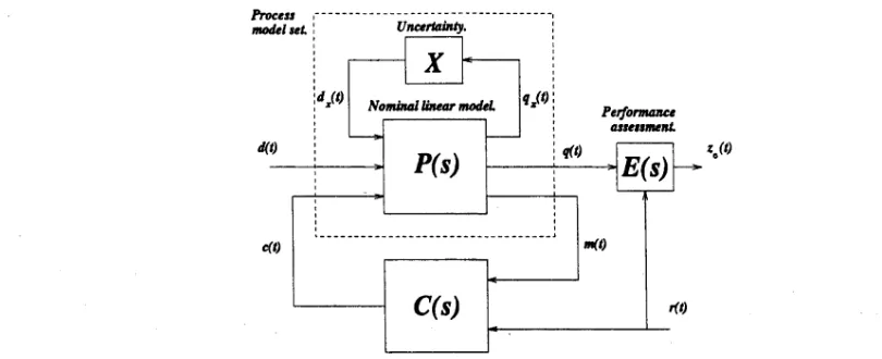
Figure 1.2 describes one means of addressing the control design task introduced in Figure 1.1. As a basis for the design of the controller, we take a nominal model P (s) of the process which is a finite dimensional linear time invariant (FDLTI) system.1 Also a FDLTI system E {s) is introduced to assess the performance of the system (note that
E(s) is chosen to reflect the designer’s objectives and does not model any part of the real process). For simplicity and ease of implementation, we also restrict our attention to the class of FDLTI control laws. This obviously rules out nonlinear and adaptive control strategies.
T h e P r o c e ss M o d e l S et V.
It is well recognized th at nominal linear models alone cannot always provide a descrip
[image:35.525.59.456.62.249.2]1.1 Control Design and Controller Synthesis. 17
Process
model set. Uncertainty.
Nominal linear model
Figure 1.2: A framework for linear control design, including a nominal linear process model P(s) with process uncertainty X (possibly nonlinear and time-varying), a linear control law C(s) (to be designed) and a lineax system E(s) (to be chosen by the designer) which generates objective signals for performance assessment.
tion of the process which is adequate for control design. For example, it is well known th a t the actual closed-loop stability of nominally high-performing lineax control designs can be very sensitive to deviations from the nominal plant model (see e.g. [34] and [26]).
In Figure 1.2, the process has been represented by a set of models V which consists of two components. The first is the nominal model P which is a FDLTI system. The second component is an uncertain dynamical system X (not necessarily FDLTI). With reference to Figure 1.2, observe th at uncertain process behaviour is attributed to the system X which maps qx (t), consisting of signals related to the nominal process model, to dx (t) which consists of signals which disturb the nominal lineax process dynamics. It is hoped th at the process can be adequately described by P (s), together with at least one X G A, where X is a set of systems which is chosen by the designer in an effort to capture his uncertainty in process behaviour. The elements P and X of the process model set V are described below in more detail.
Rem ark: A number of different ways of describing how the process uncertainty X
perturbs the behaviour of the nominal model are commonly adopted. These include multiplicative, additive and normalized coprime factor uncertainty descriptions (see e.g. [34], [69],[82] and [66]). It is generally possible to describe uncertain plant behaviour in terms of a connection of the type shown in Figure 1.2 (see [69]). □ N om in al Linear T im e Invariant P rocess M odel.
The inputs of P{s) include all process inputs (actuator signals, disturbances) as well as the the signal dx(t) which is the output of the model uncertainty. The outputs of
P{s) include all process outputs (sensor signals and performance variables), as well as the signal qx (t) which is the model uncertainty input.