I
' -·
~·
.· ...··~ ~-.,,re-- = -~ - -- ..;.i, ---.~ --- - '~ ..
-. "
·~
:r:"
A REGRESSION A__NALYSIS OF ~ENTAL HEALTH DATA
1
by u
d
ROBYN A.TTEWELL :
A1
l
r,,' u
• J
~
!
.,, ,, ( u
~·
,.II
A Case Study submitted to the Australian National University C 0 I
towards a Master of Science Degree by coursework in the I
CJ Department of Statistics, Faculty of Economics.
I~ November 1982
:
11
lo
, '.l
l 1,
·,
'C
;-r. "
'ti
II ...
I .~,
· ~
--I ~eclare this material to be my own work except where
stated otherwise .
Acl<.nowleigements
I wish to thank Paul Duncan-Jones for making this problem available as a case study and for his encouragement and
guidance 1n his capacity as my supervisor.
I also haa some useful discussions with Professor Heathcote. The C.S.C. Univac computer playe~ an important role in this work and I acknowledge i t ' s contribution to relieving the
computational burden and the task of pro~ucinq this manuscript.
·~
·- --
....
a
I • :,
I
l
I
...
C
I
IJ a
I
I
'I
.,
l
"'
:
'
' '
;
: ,r'
'
L
:, 1 1, " 1, ', ~
j
r
~?
11
-~
q
-_ase Study
1 .
2.
3 •
4 .
5 .
6 •
7 •
8.
Table of contents
Introduction to the problem
The Data and the Approac~
2 . 1. Measuri ng Disturbance
2. 2 . Social Support 2 • 3 • Z\d v er s i t y
2. 4. Method
Data Reduction
3 . 1 . Construction of Adversity and Social Support Scores 3.2 . Distributions of these scores
Single Predictor Models
4. 1 . GLM : Binomial errors
4. 2 . Multivariate GLM : Multinomial errors
4. 3. Continuation Odds Models
Testing for Interaction 5. 1. Logit link
5 .2 . Clog log link
Models involving t he original variables 6 . 1 . More Logit Models
6 . 2 . Exponential ~egression 6 . 3 . Proportional Hazards
Discussion
Bibliography
-1
-2
-3 -3 -5 -5
-6
-9
-9
-10
-14 -14 -14 -17
-19 -19 -26
-31 -31 -31 -33
-34
Case Study
1 . Introduction to the problem
This study is concerned with investigating the associations between
neurosis, a person's social contact, and exposure to adverse
circumstances. Psychiatric illnesses which are classed as psychotic,
(eg. schizophrenia), involve major functional disorder. Much researc~
has been concerned with these illnesses since data are readily
available from institutions and psychiatric consultations.
~on-psychotic illnesses such as emotional disorders, anxiety ani
depression are harder to define and recognise and are much more
widespread. It is this form of mental illness as identified in the general community that is the focus of this case study.
That there exists an association between lack of social and
personal ties and mental disturbance is generally accepted. The
direction of causality, that is, whether little social contact
contributes to neurosis, or neurotic symptoms affect an individual's social interaction, or whether they are both influenced by a third
factor(eg. personality), is still under investigation. Important and
stressful events occurring in a person's life are also recognised as
contributing to mental disturbance. But whether there is a significan~ interaction with social support is under current debate as well.
It has been shown in studies by Henderson et al (1980) and
Henderson (1981) that deficiencies in social relationships and, more
importantly, assessment of existing relationships as inadequate, are
more strongly associated with subsequent symptoms under conditions o= adversity. Brown and Harris(l978) made similar findings for the onset
of depression in women in their study.~owever ~iller and Ingham(l976)
suggest that deficiencies in social bonds act independently of life
events in the aetiology of neurotic illness. Brown et al (1975)
identified four factors influencing the effects of stressful events i~ causing depression. These were, having an intimate confidant, loss
o=
mother at an early age, having many young children at home, and lac~ of employment. However i t was admitted that a sample of 220 women 0£ whom only 10% were recent cases, is too small to determine whethersignificant interactions exist.
The investigation of interaction and comparisons between studies are made difficult by the problem of definition and measurement of t he
quantities involved. Though the data set of this study was gathered
for purposes other than an intensive study of psychiatric
epidemiology, i t does have the advantage of being large. This offers the possibility of a more definitive statement about interaction than
previous studies have provided. The main focus of the present
investigation is to determine whether a model incorporating
interaction between adversity and social support will account for
materially more of the variance in a measure of neurotic illness tha~
Case Study -3
2. The Data and the ~pproach
In 1975 the Australian Bureau of Statistics conducted a health care
survey for the Healt~ Commission of ~SW. People from aporoximately
3100 selected households in the Gosford,Wyong and Illawarra regions 0£
NSW were asked quite detai ed questions on all aspects of their health
and use of local health services. The survey was the first large-scale
household survey of morbidity and health services in Australia, and
was undertaken primarily to assess the adequacy of health services i~
these areas.
We are grateful to the NSW Health Commission for making the dat~
tapes available for secondary analysis. The data subset relevant t~
this study involved the responses to the mental health section of the
questionnaire by 6067 adults (15 years of age and over).Patients i ~
hospitals,convalescent homes and institutions were not included in t~e
survey.
Although the overall sample design involved several stages ani
sampling techniques, simple random sampling was assumed in this
analysis. Whereas the original analysis was concerned with estimation
of prevalence of neurosis, our aim is to test hypotheses about the
relationships between neurosis and other factors using techniques not
appropriate to smaller sets of data.
Results from empirical studies by Kish and Frankel(l970) for
s imilarly complex surveys have shown that the design effects computei
for estimating standard errors using balanced repeated replication
tend to be smaller for analytical statistics such as regression
coefficients compared with aggregates and means.
Another detailed study by Landis(l982) for an American survey
similar to this , has shown that effects found to be non-significant
(in regression , anova and contingency table analysis) under the
simplest assumptions are unlikely to be found significant if sampling
weights and the design structure are taken into account.
In this study, given the sample size, marginally significant
effects are of lesser scientific interest, and one would already be
cautious of interpreting them, even if assured of the validity of the
assumptions required for the significance tests.
2. 1 . Measuring Disturbance
The measure of neurosis available from the survey results was the
score obtained on the 12 item version of the General Health
Questionnaire (Goldberg 1972) , which is listed below.
Each question was answered with one of four graded responses.
These are worded according to the question but follow the same general
form . For example, the response set for question 1. is as
follows-( i ) (ii) (iii) (iv)
better than usual
same as usual less than usual
Case Study -4
General Health Questionnaire
1. Have you recently been able to concentrate on whatever you're
doing?
2. Have you recently lost much sleep over worry?
3 • Have you recently felt that you are playing a useful oart
things?
4. Have you recently felt capable of making decisions about
things?
5. Have you recently felt constantly under strain?
6. Have you recently felt that you c8uldn't overcome your
difficulties?
.
in
7 . Have you recently been able to enJoy your normal day-to-day
activities?
8 .
9 •
10.
11.
Have you
Have you
Have you
Have you person?
recently been
recently been
recently been
recently been
able to face UP to your problems?
feeling unhappy and depressed?
losing confidence in yourself?
thinking of yourself as a worthless
12. Have you recently been feeling reasonably haopy, all things
considered?
The responses were dichotomised to O for the 'normal' response
and 1 for the 'pathological' response, and then summed to give a score
ranging from Oto 12. For example, a negative response to question 8
would contribute 1 unit to the overall score. This follows the normal
scoring convention for this questionnaire. The total scores will
subsequently be referred to as GHQ scores.
Assuming that neurotic disturbance can be measured on a single
continuous axis ranging from hypothetical normality to severe
isturbance, the score is interpreted as a quantitative estimate of
the individual's degree of disturbance.The higher the score,the more
neurotic the individual.In the original analysis for the Health
Commission a score of O or 1 was taken to be normal.
Extensive validation studies have been carried out on the 60 ana
30 item versions of this questionnaire, and justification of its form
and content as an instrument for measuring non-psychotic disturbance
is discussed at length in Goldberg(l972). It is shown that the 12
questions chosen for the smallest version have the best discriminatory
power .
The GHQ shares shortcomings with other self-administered
questionnaires in depending on the individual to understand the form
of the questions and answer them accurately. By continually referring
to a person's cu~rent state, chronically disturbed people may not
score highly enough to be distinguished from the normal people. It is
already popular, however, and its advantages include its ease of use,
Case Study -5
2 . 2 . Social Support
The 9 questions of the survey selected for a social bonds measure
are listed below. The possible responses were 0, 1-2, or 3+.
Questions Pertaining to Social Support
1 . How many people (friends,family or neighbours) would you find
i t easy to call on for PRACTICAL help in an emergency or
crisis ?
2 . How many people would you find it easy to call on for
EMOTIONAL help in an emergency or crisis?
3 . How many times in the past week would you have talked to or
corresponded with any of your RELATIVES not living with you?
4 . Bow many times in the past week would you have talked to your
~EIGHBOURS?
5. How many times in the past week would you have talked to or
corresponded with your FRIENDS?
How many times have you attended or participate1
activities in the past month?
.
in
6. SOCIAL or LICE~CED CLUB (e.g. Leagues or R.S.L.)?
the following
7. SPORTING or RECREATION group (e.g. team member or organiser)?
8. CHURCH SERVICE or MEETING?
9 . any other COMMUNITY SERVICE, SPECIAL INTEREST GROUP or UNION
MEETI~G (e.g . APEX, hobby class, school p. & c.)?
The answers to these questions (SS1 - SS9) convey information on
the amount of interaction a person has with friends, relatives,
neighbours , and the extent of participation in community activities.
These are fairly crude measures, especially when compared with the
detailed Interview Schedule for Social Interaction (Henderson, Byrne,
Duncan- Jones 1981), which goes much further than 'counting heads' and
includes personal assessments of the adequacy of frieniships and
social integration . However they appear adequate in the context of
this large multi- purpose survey.
2 . 3 . Adversity
Life events are defined as events which occur in a person's life
which may cause stress . They usually involve significant changes in
health or way of life. The survey included a list of 36 life events
(e .g . marriage,divorce,death in the family,moving house,major physical
illness , loss of job etc . ) Each individual was required to indicate
Case Study
(i) in
(ii) (iii) (iv)
the last 2 months
3- 6 months
7- 12 months
12-24 months
-6
Information of this kind is highly susceptible to recall error
and since i t is not each particular event that we are intereste~ in,
the information was summarised into 4 life event variables
representing the total number of life events recalled by a person for
each time period . These are subsequently referre~ to as LE1,LE2,LE3
and LE4 .
With this construction each life event is given equal weight
within each time ?eriod, yet i t is plausible that some events may have
more impact than others and some individuals may place more importance
on particular events depending on their sex, age, social class or
cultural background . The concensus of the current literature is that
simple frequency counts of life events are inaoequate measures of
adversity and many methods have been proposed to best quantify their
impact. However, no additional information was available in these
survey results on the reactions of each individual to experiencing the
events.
2.4. Method
The correlation structure of the variables indicated the general
trend of relationships between these measures. Over the 6067
individuals , positive correlations were observed between GHQ score and
all 4 life event variables (max 0.13
ior
LEl), and negativecorrelations for GHQ score and all 9 SS variables (-0.12 for
SSS-friends) , giving support to the basic hypotheses of associations
between neurosis, the occurrence of stressful life events, and lack of
social contact .
As this is a cross- sectional study, we cannot investigate the
direction of causality. In the following regression analysis GHQ score
will be modelled as the response variable, but i t is recognised that
neurotic symptoms may also influence a person's social behaviour, or
cause events such as marriage breakup or loss of one's job.
A multiple regression of GHQ score on the 13 variables could
explain only 7% of the variance and examination of the fit revealed
that for large GHQ score the residuals were large and positive and
became smaller with decreasing GHQ score. This may be attributed to
the skewness of the distribution of the scores as illustrated by the
Case Study
Table 2-1. GHQ Score Frequencies
GHQ score Frequency % of Total
0 3791 62
1 841 14
2 460 7.6
3 300 4.9
4 192 3. 2
5 128 2. 1
6 100 1.7
7 72 1. 2
8 51 . 71
9 43 .71
10 33 .54
11 32 .53
12 24 .40
6067
The subsequent analysis tries to accommodate for this by
(i) selecting a threshold GHQ score to classify an individual as
either normal or a case and using logistic regression techniques
(ii) dividing the GHQ score into several contiguous ordered categories
and using a multivariate analogue to Generalised Linear ~oaels as
described by McCullagh(l980). Then parallel logistic regression lines
are fitted with intercepts dependent on the category bounds.
(iii) modelling the counts in the 13 categories of GHQ score directly
using exponential regression or using the (discrete) proportional
hazards non-parametric approach of survival analysis.
In order to obtain a workable model for testing both general main
effects and the interaction between social bonds and adversity, the
information in the 4 LE and 9 SS variables was condensea into a single
LE score and a single SS score for each individual. These scores were
then divided into several contiguous categories and cross-classified
with GHQ score to form 2-way tables for testing for main effects
separately, and 3-way tables for testing between adaitive and
interactive models. The next chapter explains in more detail the
construction of the scores.
The analysis of each main effect using the aichotomous and
multi-response models is treated in Chapter 4 and Chapter 5 contains
the results of testing for interaction. In Chapter 6 the original
variab es are considered separately and the thira approach is
[image:10.802.13.774.20.1137.2]4000
3600
3200
-2800
-2400
-
>-~
2000-w
:::> 0
w
er:
LL l 600
-l 200
800
400
--8
PLOT 2.
1
D
I
S
T
R
I
B
U
T
I
ON
OF
GH
Q S
COR
E
o.oo
2.00 4·.00 6.00s.oo
10.00 12 .00Case St dy -9
3. Data Reiuction
3.1. Construction of Adversity and Social Support Scores
~ single adversity score for each iniividual was obtained by using the regression coefficients from the multiple regression of the raw GHQ score on the 4 LE variables. The weights for a social supoort score based on the 9 SS variables were obtained on a similar but separate regression. Table 3-1 lists the estimated coefficients.
Table 3-1. Weights Used to Form LE and SS scores
Variable Est . reg. coeff. Variable ~st. reg. coeff.
constant .81 constant 3.6
LEl 0- 2 months .25 SS5 friends -.27
LE4 12-24 .11 SS2 emot. help -.20
LE3 7-12 .16 SS7 rec. group -.16
LE2 3- 6 .09 SS6 clubs -. 14
SS8 church -.13
SS4 neighbours -.08
SS1 prac. help -.1 2
SS9 comm. groups -. 03
SS3 relatives -.02
The order of inclusion of the variables was determined by the respective contribution of each variable not already in the equation, to the explained variance if added. Hence i t can be seen from Table 3-1 that the number of most recent life events(LEl) and the number of
friends(SS5),respectively are the most important in the two
regressions. The number of people one can call on for practical
help, (SS1) is well down on the list, but this variable is highly
correlated (.5) with SS2.
The amount of explained variance is onl y 2.8% and 3.4% for life events and social support respectively, and again there is a mar~ed relationship between the residual s and the predicted values. Some of the regression coefficients are quite small and yet one cannot depend
on F ratio tests to render them non-significant as the normality
assumptions are not valid.
Despite this i t is believed that the resulting measures of
conditions of adversity and social contact obtained by using these
weights to get total scores, will provide at least initially adequate summary indices for the task at hand: ie . to assess whether there is an interaction between
.
these two factors in their association with neurosis .There are several approaches that could have been taken at this stage. Due to the skewness of the GHQ score distribution, the method of functional least squares (Heathcote 1982) was also consiiered. It
is an extension of the normal least squares regression with minimum
restrictions on the error distribution (no symmetry or moments
required). A family of slope estimates indexed by a real parameter t, is obtained by minimising the empirical cumulant generating function of the error distribution. A choice of t=O gives the usual least
squares estimates and is optimal for normally distributed errors ,
[image:12.810.15.777.2.1136.2]Case Study -10
with respect to least sq ares. Applied to this data set the procedure
confirms the lack of normality but the convergence is slow and the
resulting coefficients are extremely small and not readily
interpretable. This is most probably due to the discrete nature of the data, especially the 3 value range of the SS variables, and justifies the contingency table approach discussed in subsequent chapters.
A drawback to the use of factor analysis at this stage, and selecting a single LE factor and a single SS factor is that some
aspects of the data may be overlooked, which are important in
accounting for the association with the dependent variable. Providing the tvo sets of variables are orthogonal the separate regression scores should prove suitable . The data supports this with the absence of significant correlations between the 4 LE variables and the 9 SS variables. Of these 36 correlations the two 'largest' are -.06 between
LE2 and SS4 (neighbours), and 0.05 between LE4 and SSl (emotional
help) . One may have expected LEl to be the most likely to have an association since the social support questions were specifically about the previous week and month.
A more formal check of independence was made by calculating the canonical variates for these two sets of variables (ie. finding the two linear combinations of each set which maximises the correlation between the scores). The computations gave a life event canonical
variate which could explain only 1% of the variance of the social
support canonical variate (an0 vice versa).
Further evidence for orthogonality was given by the increase in R squared (regression ss/ GHQ ss) remaining at about 0.03 when the four LE variables were included in the regression, whether the nine SS variables were in the equation or not.
3 • 2 • Distributions of these scores
The scores were divided into nine equal sized cat~gories so that the minimum and maximum defined the lowest and ~ighest bounds. Their distributions over the whole data set are indicated by the frequency table (3-2) and plots (3 .1,3.2).
The sKewed nature of the LE score reflects the sKewness of both the GHQ score distribution and the distibution of the 4 LE variables. Most people recorded few life events occurring in each time period. In fact about 55% of the sample recorded no life events for- 1 to 2 years and about 69% for each of the other time periods. The skewness parameters for the categorised forms of the LE and SS scores are 2.4 and .39 respectively, compared with 2.6 for GHQ score.
The SS score should be thought of more as a 'lack of contact' score since fewer friends and less social participation result in a higher numerical value of the score. Compared to the four ISSI scores
,ase Study -11
Table 3-2. LE and
ss
score FrequenciesLE Interval '1idpoint Frequency
ss
Interval Midpoint Frequency0 .81, 1 . 16 0.99 3880 0 . 13 , 0.39 0.26 79
1.16,1.51 1.34 1406 0.39,0.65 0.52 511
1.51 ,1.86 1.69 498 0.65,0.91 0.78 1130
1.86,2.21 2.04 174 0.91,1.17 1.04 1772
2.21,2.56 2.39 64 1.17,1.43 1.30 1237
2.56,2.91 2.74 29 1.43,1.69 1.56 710
2.91,3.26 3.09 6 1.69,1.95 1.96 418
3.26,3.61 3 .44 8 1.95,2.21 2 .08 179
3.61,3.96 3.79 2 2.21,2.47 2.34 31
-12
PLOT 3.
HISTOGRAM OF
L
FEE ENT SCORES
4000
3600
3200
2800
-_J
<
>
a::
w
I
-2400
-z
w a::
0
u
U)
2000
-w
_J z
>- \ 600
-u
z.
w
::>
-0
w a::
LL 1200
800
400-0 I 1
11---,
I I I l 1 l I I I I I
0. 00 1 . 00 2.00 3.00 4,00
s
.
oo
.
6.00- 13
PLOT 3.2
H
I
STOGRAM OF SOC
IAL
S
UPPO
RT S
CORE
S
4000
3600
3200
2800
_J
< >
n::
w
I
-2400
z
w
n::
0
(.)
Cf)
2000
Cf) Cf)
z
>- \600
(.)
z
w .::>
0
w
n::
LL 1200
800
400
0 ~_.._r--~_.._----'-r__.__~...L-;---...---.r---r----.--- - - -- ~ - ~----.
o.oo
\ . 00 2,00 3.00 4,00 5.00 6,00Case Study -14
4. Single Pre1ictor Models
4. l . GLM : Binomial errors
We have seen that the normal linear regression moiel could not
adequately describe the data and the oroblem lies with the skewed
nature of the distributions. The GHQ scores are now interprete~ as
indicating a case, or not, according to a chosen threshold score(9).
The number of cases are assumed to follow a Binomial ~istribution with
the mean dependent through a link function on some linear combination
of explanatory variables. LE and SS scores are used as predictors in
separate regressions in this chapter.
Using the logit link and defining q(x)=Pr(GBQ score> 8
I
X=x)the model is
log[q(x)/ (1-q(x))J =A+ Bx ( 1 )
This model is saying that the log odds that an individual is a
case is a linear function of the explanatory variable, and unit change
in this variable produces unit change in the log odds ratio.
The computer package GLIM (qelAase 3) was used to fit the model,
using iteratively reweighted least squares to obtain the maximum
likelihood estimates of the parameters.The GLM theory of Nelder and
Wedderburn(l972) shows how the reductions in deviance as parameters
are added to the model are approximately Chi-squared and for binomial
errors the deviance or likelihood ratio can be used as a goodness of
fit statistic.
With a threshold GHQ score of 2 and the explanatory variable
taking the values of the midpoint of each a~versity score interval,
model (1) gave a deviance of 6.31 on 7 degrees of freedom with slope
0.88. Using SS score a deviance of 6.21 (again on 7 df) was obtained,
with slope 1.01 The direction of these regression lines is consistent
with the basic hypotheses since a higher LE score indicates more
severe conditions of adversity and a higher SS score reflects less
social contact, according to the coefficients in Table 3-1.
Despite these fits being reasonably good, by choosing a single
threshold, much of the information available is being ignored. It also
seems more appropriate to assess neurotic disturbance by ~egree,
rather than by an arbitrary definition of presence or absence.
4. 2. Multivariate GLM: Multinomial errors
Mccullagh has developed a multivariate extension to ~elder and
Wedderburn's theory involving a multi-response dependent variable with
ordered categories. The categories need only be contiguous and have no
size constraints . The GHQ score is now grouped into 5 categories as
indicated in the 2-way frequency tables(4-l and 4-2). These show the
cross classification of (the categorised forms of) LE an~ SS score
[image:17.809.21.774.0.1142.2]_ase Study
Table 4-1 . LE score by G:-1Q score frequencies
GHQ score
LE interval 0 1 2 3 .. 4 5 .. 12
mio-point
.99 2648 475 243 267 247
1.34 789 231 130 126 130
1.69 237 88 53 56 64
2 .04 81 29 20 18 26
2.39 25 10 9 14 6
2.74 10 5 3 5 6
3.09 0 1 0 4 1
3.44 1 2 1 2 2
3.79 0 0 1 0 1
Total 3791 841 460 492 483
Table 4-2.
ss
score by G:-1Q score frequenciesGHQ score
ss
interval·o
1 2 3 .. 4 5 .. 12mid-point
.26 62 9 4 3 1
.52 365 72 30 26 18
.78 787 136 76 80 51
1.04 1151 240 141 128 112
1.30 721 190 95 121 110
1 . 56 401 109 56 63 81
1.82 212 58 39 41 68
2.08 74 24 17 27 37
2.34 18 3 2 3 5
Total 3791 841 460 492 483
Define pj(x)=Pr(GHQ score lS
. .
in any category 1 .. jlX=x) l<=j<5=Pr(GHQ score <= ej
I
X=x)Then the Proportional Odds model lS
.
thatlog[pj(x)/(1-pj(x))J - Aj
-
Bx l<=j<S-15
Tota_
3880 1406 498 174 64 29 6 8
2
6067
Tota2..
79 511 1130 1772 1237 710 418 179 31
6067
( 2 )
'tv!odel ( 2) is just
a
multi variate form of ( 1) with mul tino, ialv~riation instead of binomial errors. Mccullagh has written a c~mputer
pacKage (called PLUM) which estimates the parameters by ~aximu~
liklehood in a manner analogous to GLI~. With the linear structure of
mo el (2), 4 parallel logit regression lines are fitted with
intercepts dependent on the cutoffs .
It is noted that these models can be fitted within the current framework of GLIM by using the $OW directive to define a composi~e link function, and that this is one of the new features facilit~ted in the next version of GLIM. (Thompson, Baker 1981)
Significant reductions in deviance were observed in fitting model
(2) with LE and SS score category midpoints as the explanatory
variable . The deviances were 37 .0 and 41.7 both on 31 df, compared with 207 and 208 on 32 df respectively for a model with B=O.
[image:18.800.15.776.73.1142.2]..
Case Stu y -16
table of parameter estimates (4-3). This shows the results of fitting
model (1) four times with the threshold GHQ score at the four
different cut-off points. Note that the intercepts decrease as the
threshold increases. The sign difference between the estimates of A
and Aj are due to the definitions of q(x) and oj(x) .
Note the (opposite) trends in the estimated slopes for model (1)
as threshold increases.(See also plots 4.1 (~) and (b)). The
Mccullagh model is assuming these are constant an~ the estimates of B
for model (2) are closer to the estimates for model
(1)
at the lower thresholds since 76% of the observations fall into the first two GHQscore categories. The aoproximate 95% confidence intervals estimate~
for the slooes do not cover the range given by model (1), so the
proportional odds model may not be the best summary of the data.
Table 4-3 . Comparing .~odels (1) and (2)
Model ( 1)
Threshold 0 1 2 4
LE A -1.78 -2.34 -2.73 -3.42
B DEVIANCE DF 1.07 14.6 7 .964 7.77 7 .882 6.11 7 .792 7.32 7
ss
A - 1.38 -2.20 -2.87 -4.01B DEVIANCE DF .748 8.12 7 .874 6.34 7 1.01 6.24 7 1.27 2.79 7
A mode l called the proportional
replacing the log odds in model
transformat ion .
log[- log(l-pj(x))J
=
Aj - Bxcutpoint 0
Aj B DEV DF Aj B DEV DF 1.68 1.46
Model (2)
1 2.26 .974 37.0 31 2.14 .830 41.7 31 2
2 . 85
2.63
4
3.66
3.44
hazards model is obtained by
(2) by the complementary log log
( 3 )
Whereas previously pj(x) was modelled as the logistic distribution
f unction , model(3 ) is equivalent to
pj(x)
=
1 - exp (-exp(Aj - Bx))Now the ratio, log(qj(xl)/ log(qj(x2) , instead of the odds ratio, is
assumed constant over categories, and depends only on the difference
between the covariate values.
[image:19.799.20.772.20.1139.2]Case Study -17
However by noting that the C-log log transformation is asym~etric and
reversing the order of GHQ score categories in table 4-1, (effectively replacing p by q) , a deviance of 35 . 3 was obtained. The differences in fit are explained by comparing the graphs of slope estimates for the bivariate response models with logit and cloglog links (at
different thresholds) . The improved fits of the proportional ~azards model are reflected by the estimated slopes being more nearly constant over the different thresholds . See Plot 4.1 (a to f). · The deviance
for the corresponding Mccullagh model is shown in brackets on each graph .
4. 3 . Continuation Odds Models
~nother technique for modelling or~inal multivariate responses is
to fit model
(1)
at the series of different thresholds but truncating the sample each time at the previous lowest (or highest) threshold. This is equivalent to conditioning on G9Q score being greater than(lower truncation) , or less than (upper truncation) a particular value.
Models (4) and (5) describe two sets of continuation ratios.
log [(P(GHQ score> j)/(P(GHQ score - j) ~+Bx
log [(P(GHQ score < j)/(P(GHQ score -
j) -
A+ Bxj=0,1,2,3,4
j=4,3,2,l
( 4)
( 5 )
Fienberg (1977) discusses these models and shows that the individual Chi- square statistics for each model can be added to obtain an overall goodness of fit statistic for the series.
Such models have aims similar
io
the Mccullagh models and theproportional hazards models, and in this study give more insight into
the diff erences between the associations of LE and SS with GHQ score. Model (4) fitted quite well at the lower thresholds, but once
people with GHQ scores of O and 1 were excluded from the data, the linear relationship between log odds (GHQ score> threshold) and LE
score was lost. It was maintained in the model (5) top truncated
series .
Both models (4 ) and (5) proved suitable with SS substituted for
x. The increasing trend in slope with increasing threshold,
-18
PLOT 4.1
S opes est meted for ( oglt and cloglog) models with 4 different
thresho l d def i nit i ons of q ( x )
( C ) log [q{ X )/p( X ) ] •a+~LEXLE ( b ) l og [q( X )/p( X ) ] ·a+~ ssx ss
l. 2 l . 2
!;2
1. 0 l . 0
0.8
37
0.8~LE
~ss
0.6 0.6
0.4 0.4
0.2 0.2
0.0 0.0
0
8
08
( C ) I og- [ I og( 1-p( x)) ]-a+ ~LExLE ( d ) l o g - [ I o g C 1 - p ( x ) ) J-a+~ ss x ss
I. 0 1. 0
0.8 0.8
i3L
E
--Pss
0.6 0.6
I
~
0.4
7{
0. 4-0.2 0.2
0.0 0 .0
0
8
08
C e ) I og- [ I og( 1-q( x)) J-a+ ~LExLE ( f ) I o g- [ l o g ( 1 - q ( x > > J-a+~ ss x ss
1 . 2 1. 2
b
O
1. 0 1 • 0
0.8 0.8
~LE
0.5
35
~ss
C, . 6
0.4 0.4
C,. 2
II. 2
~
0. C, (L 0
l
2
4
~ase Study -19
5. Testing for nteraction
5 . 1 . Logit link
In fitting additive and interactive rno~els, the regressors (LS
and SS) were treated as either a covariate with values being the
midpoint of each category (as before), or as a 3 level factor(by
combining 3 sets of 3 consecutive categories). In the tables of
results the small letter f will indicate the factored form of the
variable. For example the proportional odds model SSf + LE fits
parallel logit regression lines with interceots depending on the
cutoff points and level of SS score, with slope determined by the
linear association between the logit of GHQ score and LE category
midpoint . The interactive model allows the slope to vary accoriing to
SS level.
The results of the two 3-way classifications (LE by SSf by GHQ
and SS by LEf by GHQ) are listed in tables 5-1 and 5-2 and were used
as inout to the PLU~ program. Note that iespite the initial large data
set, only 24 of the 27 possible rows are non-zero an~ approximately
half the entries in each table are less than 5. This· may affect the
the distributional properties of the final deviance, but should not
~ase Stuiiy -20
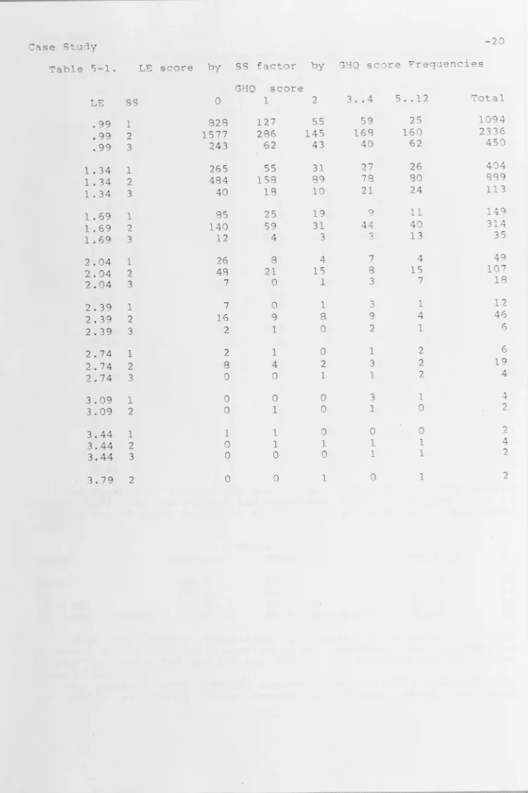
Table 5-1. LE score by
ss
factor by GHQ score FrequenciesGHQ score
LE
ss
0 1 2 3 .. 4 5 .. 12 Total.99 1 828 127 55 59 25 1094
.99 2 1577 286 145 168 160 2336
.99 3 243 62 43 40 62 450
1.34 1 265 55 31 27 26 404
1.34 2 484 158 89 78 80 889
1.34 3 40 18 10 21 24 113
1.69 1 85 25 19 g 11 149
1.69 2 140 59 31 44 40 314
1.69 3 12 4 3 3 13 35
2.04 1 26 8 4 7 4 49
2.04 2 48 21 15 8 15 107
2.04 3 7 0 1 3 7 18
2.39 1 7 0 1 3 1 12
2.39 2 16 9 8 9 4 46
2.39 3 2 1 0 2 1 6
2.74 1 2 1 0 1 2 6
2.74 2 8 4 2 3 2 19
2.74 3 0 0 1 1 2 4
3.09 1 0 0 0 3 1 4
3.09 2 0 1 0 1 0 2
3.44 1 1 1 0 0 0 2
3.44 2 0 1 1 1 1 4
3.44 3 0 0 0 1 1 2
[image:23.795.18.768.17.1143.2]Case St ,jy
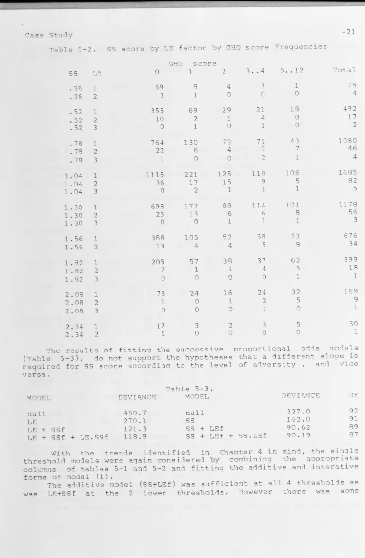
Table 5-2. SS score by LE factor by ~HQ score Frequencies
ss
LE.?6 1
.26 2
.52 1
.52 2
.52 3
.78 1
.78 2 .78 3
1.04 1 1.04 2 1.04 3
1.30 1 1.30 2 1.30 3
1.56 1
1. 56 2
1. 82 1
1. 82 2 1. 82 3 2.08 1
2.08 2 2.08 3
2.34 1
2.34 2
GHQ score
0 1 2
59 3 355 10 0 764 2?. 1 1115 36 0 698 23 0 388 13 205 7 0 73 1 0 17 1 8 1 69 2 1 130 6 0 221 17 2 177 13 0 105 4 57 1 0 24 0 0 3 0 4 0 29 1 0 72 4 0 125 15 1 88 6 1 52 4 38 1 0 16 1 0 2 0
3 . . 4
3 0 21 4 1 71 7 2 118 9 1 114 6 1 58 5 37 4 0 24 2 1 3 0
5 .. 12
1 0 18 0 0 43 7 1 106 5 1 101 8 1 73 8 62 5 1 32 5 0 5 0 -21 Total 75 4 1080 46 4 1685 82 5 1178 56 3 676 34 399 18 1 169 9 1 30 1
The results of fitting the successive proportional odds models
(Table 5-3), do not support the hypotheses that a different slope is
required for SS score according to the level of a~versity, and vice
versa.
~ODEL
null LE
LE+ SSf
LE+ SSf + LE.SSf
Table 5-3.
DE IANCE MODEL
450.7 null
270.1
ss
121.3 SS + LEf
118.9 SS + LEf + SS.LEf
DEVI~KfCE 327.0 162.0 90.62 90.19 DF 92 91 89 87
With the trends identified in Chapter 4 in mind, the single
threshol models were again considered by combining the appropriate
columns of tables 5-1 and 5-2 and fitting the additive and interative
forms of model (1).
The additive model (SStLEf) was sufficient at all 4 thresholds as
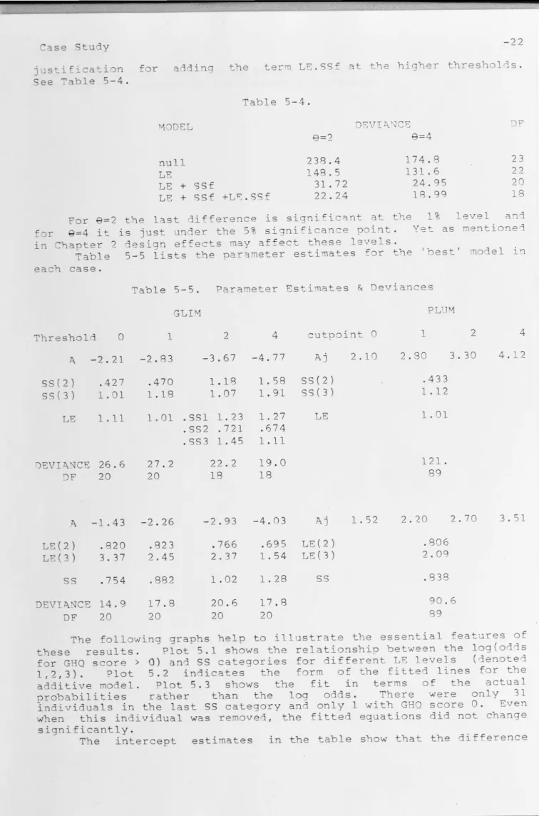
[image:24.795.14.762.0.1143.2]ase Study -22
justification for adding the term LE.SSf at the higher thresholns.
See Table 5-4.
MODEL
null LE
LE+ SSf
Table 5-4.
8=2
LE+ SSf +L~.SSf
238.4 148.5
31.72 22.24
DEVI"A.~CE
8=4
174.8 131.6
24.95 18.99
23
22
20
18
For 8=2 the last difference is significant at the 1% level and
for 9=4 i t is just under the 5% significance point. Y~t as mentione~
in Chapter 2 design effects may affect these leve s.
Table 5-5 lists the parameter estimates for the 'best' model in
each case.
Table 5-5. Parameter Estimates & Deviances
GLIM PLUT\1
Threshold 0 1 2 4 cutpoint 0 1 2 4
A - 2.21 -2.83 -3.67 -4.77 Aj 2.10 2.80 3.30 4.12
SS(2) .427 .470 1 . 18 1.58 SS(2) .433
SS(3) 1.01 1 . 18 1.07 1 . 91 SS(3) 1.12
LE 1.11 1.01 .SS1 1.23 1.27 LE 1.01
.SS2 .721 .674
.SS3 1.45 1.11
DEVI "A.NCE 26.6 27.2 22.2 19.0 121.
DF 20 20 18 18 89
A -1.43 -2 . 26 -2.93 -4.03 Aj 1.52 2.20 2.70 3.51
LE(2) .820 .823 .766 . 69 5 LE(2) .806
LE(3) 3.37 2.45 2.37 1.54 LE(3) 2.09
ss
. 754 .882 1.02 1.28ss
.838DEVI~NCE 14.9 17.8 20 .6 17.8 90.6
DF 20 20 20 20 89
The following graphs help to illustrate the essential features of
these results. Plot 5.1 shows the relationship between the log(odds
for GHQ score> 0) and SS categories for different LE levels (denoted
1,2,3). Plot 5 . 2 indicates the form of the fitted lines for the
additive model. Plot 5.3 shows the fit in terms of the actual
probabilities rather than the log odds. There were only 31
individuals in the last SS category and only 1 with GHQ score 0. Even
when this individual was removed, the fitted equations did not change
significantly.
[image:25.794.12.768.0.1144.2]Case Study
between the fitted lines for LE levels 2 and 3, threshold 0 , decredses as the threshold increases.
-23
Plo 5. 1
3.00
2. p, q 2.7G 2.64 2.52 2. 40
2.28
2 . 16
2.04
1. 92
1. 80
1. 68
1 • 5G 1 • 4 4
1. 32
1.20
1.
oe
.960
.840
.720
• QC)
.
~so
.360 .240
. 12
.000
- . 120
- .240 -.3GO -. 480 -.600 -. 720 -. 840 -. 960
-1. 08
-1. 20
- 1. 32
-1. 44
-1. 56
3.48 3.36
3.24
3. 12
3. 00
2.88
2.76 2.64 2.52
2.40
2.28
2. 16
2.04
1 • 92 1. 80
1. 68
1. 5 1 • 4 4 1. 32 1. 20 1. 08 .960
· . 840
.720 .600 .480
.360 .240
. 120
.000
- . 120
-.240 -. 360 -.480 -. 600 -. 720 -.840 -.960
-1. 08
-1. 20
.
bs Log aas (G~Q
>
0) Vs S score midpoir,t ( , 2, 3=LE+ levels)') J 3 3 2 2 2
2 1
2
1
1
2 1
1 1
2 1
1
2
· · · ·
·
6
:
26
···
a
:
52
·
·
o
:
is···;: o4 ·
·
1:
30
·
· ·;: 55
·
·;:
26
·
· ·
2:
oe
.
· ·
2:
32Plo
.
5.2
cff
r
%
P;--edictea .Log Oaas(GYO
>
0) Vs SS sco:e mia~oir.t% a1 /n a1 I a I
"' f
···o:25···0:52·
·o:
1s
· ··;:
04
··;:3
0··
·;:55
··,:
s5···2
:
os··2
:
32
-25
PLOT 5.3
(
1 ,
2, 3 -
L
E.f
I
e
v
e
I
s
)
1. 0 - 3 3 3
0. 9 - 2
0. 8
-o.7
-,-_
0
I\
w
20:::: Q.6
-0
u
2U)
0
I
o.5
(!)
-'-"
m
,
0
0:::: 2
CL 0,4
-0. 3
-2
0. l
-o.o
o.oo
0,40 0.80 1 . 20 1 . 60 2.00 2.40 2.80Case Study -26
Plots (5 .4,5.5) and (5.6,5.7) show the observed log odds and the fitted interactive models for 8=2 and 8=4. (~ow LE is the horizontal
axis and 1,2,3 refer to the SS levels). The last 3 LE categories contain only 6,8 and 2 individuals, but removal of the marked point
(in 5.4) didn't influence the fit significantly. Their pattern
changes consiierably with threshold.
The crossing of the lines was not expected. The steep slope at SS
level 1 may be attributed to people who scored high in the GHQ and
have few frie~ds exaggerating their degree of social contact for reasons of social desirability. Also, i t may be, that one or two close friends may provide the better support than a greater number,
especially in time of crisis.
Some indication of the type of interaction we are looking for is
evident in Plot 5.6 with thres~old 4. The first 4 points at eac~ 3 SS
levels define 3 lines with slope increasing in magnitude as SS
increases throug~ 1 to 3. However at the higher LE categories where
the odds are based on a smaller number of people, this pattern is
lost. Though the point at SS level 1 at the lowest LE category does
not readily conform to this patern, i t is not surprisincj that this point is so low since the people in this category have experienced no
life events in the last 2 years and have a lot of social contact .. The
general trends may be better described by collapsing the tables s t i l l
further (ie. to 3 SS ana 3 LE levels)
Nine points will hardly substantiate a model, but the results at
the different thresholns are listed in Table 5-6.
THRESHOLD MODEL DF
SSf + LE 5 SSf + LE +SSf .LE 3
Table 5-6.
0
5.45 5.41
1
3.86 1.80
2
10.7 1.61
4
2.34
0.413
This indicates as the plots of log odds (5.8 to 5.11) do, that the
aiditive monel is adequate except with a definition of a case as an
individual with GHQ score greater than 2.
Note that in Plot 5.11 the liries do not cross and the log odds
for GHQ score> 4 at SS level 2 remain higher than for SS level 1.
5 . 2 • Clog log linK
Similar results were obtained when the complementary log log link
was used. Small improvements were noted in the deviance values when
the categories were ordered appropriately, but there were no
appreciable differences in the trends as terms were added.
'Significance' for an interactive term was only achieved in the model LE+ SSf + LE.SSf at a threshold of 2 and again the difference in
slope at SS level 2 did not conform to a readily interpretable
[image:29.809.13.766.24.1147.2]Plot 5. 4 Obs Log Oaas(GHQ
>
2) Vs LE score midpoint C 1 , 2 , 3 =s st
1 eve 1 s)1
3
2.88
2.72 2.56 2.40 2.24 2.08 1 . 92
1 • 76
1. 6G 1 . 4 4
1 • 28
1 . 12
.960 3
.800
.640
.480
.320
. 160
.000 - . 160
-. 320
-.480 -.640 -.800 -.960 - 1 . 12
- 1 . 28
- 1 .44
-1 .6G
- 1 . 76
- 1 . 92 -2.08
-2.24
-2.40
-2.56
-2.72
2.40
2.28 2. 16 2.04
1. 92
1 • 80
1 • 68
1 • 56 1 • 4 4 1 • 32
1 • 20
1 • 08
. 960
.840 .720 .600 .480 .360 .240
. 120
.OGO - . 120
-.24G -. 360 -. 480 -.6GO -.720 -. 840 -.960 - 1 .08
-1.20
- 1 .32 -1. 44
- 1 . 56 - 1 .68
-1.80
- 1 . 92
-2.G4
-2. 16
-2.28
-2.4G
-2.52
3
3 1 2 2 2
3
3
1
2 2 2
3 12
2
2
1 1
1
~
1
. .
.
. . .
.
.
.
.
. .
.
. .
.
.
.
.
.
.
. .
.
. .
.
.
.
. .
.
.
.
.
.
.
. .
.
.
.
.
.
.
. .
.
.
. . .
.
.
.
.
.
.
. .
. .
.
.
. .
.
..
Plot 5.5
.
.
.
.
.
.
.
.
.
.
.
.
0.99 1.34 1.69 2.04 2.39 2.7 3.09 3.44 3. 7
9
%
Predicted Log Jads(GHQ
>
2) Vs LE score midpoint% % % % 2 % % % % %
.
.
. .
.
.
.
.
.
.
.
.
.
. .
. . .
.
.
.
.
.
. .
.
. .
.
. .
.
.
.
.
.
. .
.
. .
.
. .
.
. .
.
.
.
.
.
.
.
.
.
.
.
.
.
.
.
.
.
.
.
.
.
0.99 1.34 1.69 2.04 2.39 2.74 3.09 3.44 3.79
Plot 5.6
.GGG
- • 1 GG
-.2GG -.3GG -.4GG -.5GG - .6GG
-. 7GG -. 8GG
-. 9GG - 1 .GG
- 1 . 10 - 1.20 - 1.30 - 1. 4G
- 1. 5G
- 1 .50
- 1.7G
- 1 .8G
- 1.9G -2.GG -2. 10 -2.2G
-2. 3G -2.4G
-2.5G -2.6G -2.70 - 2.8G -2.9G -3.G0 - 3. 1 G
- 3.2G
- 3.30 -3.4G -3.5G
-3.6G
-3.7G
Obs Log Odos(GHQ
>
4) Vs LE scor~ 11~dpoint ( ,2, 3=SSf level s)3 3 3 2 2 1 2 1 1 3 2 1 3 1 2
3 3 2
1
1 2
2
2 1
.
. .
.
.
.
.
.
.
.
.
.
.
.
.
.
.
.
.
.
.
.
.
.
.
.
.
.
.
.
.
.
.
.
.
. . .
.
.
.
.
.
.
.
.
.
.
.
.
.
.
.
. . .
.
.
.
.
.
.
. .
.
.
. .
G.99 1.34 1.69 2. G4 2.39 2. 74 3.G9 3.4~ 3.79
Plot 5.7 Predicted Log Odds(GHQ
>
4) Vs LE score midpoint% .96G
.84G
. 72 G
.6GG .48G . 36G
.24G . 12G
• GGG
- . 120
-. 240 - .360
-. 480
- .6GG - .72G -. 840 - .96G
-1 . 08
-1 .20
- 1.32
- 1 . 44
- 1. 56
- 1. 68
- 1.80 - 1.92
-2. 04 -2. 16
- 2.28
-2.4G
-2.52
-2.64 -2.76
-2.88
-3.0G -3. 12
- 3.24
-3.36
-3.48
% % ? % %
.
.
.
.
.
.
.
.
.
. ·6
:
§§
··
·~
:
§4···~
:
i§·
·
·~
:
64".
·~:§§" ··~:i4···§:6~·
··§:44· ··§:t~··.
-29
Plo 5.8 0 slog oaas (GYQ >O) Vs LE~ ( 1 , ? , ~ = S S.f 1 eve 1 s )
3.84 3. f
e
3.52 2
3. 36
3.20
3.04
2.88
2.72 2.56
2.40
2.24
2.03
1. 92
1. 76
1 • 60
1. L4 4
1. 28
1. 12
. 960
. 800 3
.640
.480
.320 2
. 160
.000 3
- . 160 1
-. 320
-. 480 2
-.640
-. 800
-. 960 1
- 1 • 12
.
.
.
. .
.
.
.
.
.
.
.
.
.
.
.
.
.
.
.
.
.
.
.
.
.
.
.
. .
. .
.
.
.
.
.
.
.
.
.
.
.
.
.
.
.
.
.
. . .
1.4 2. 4 3. 4
Plot
5
.
9
Obs log oaas (GYQ >1) Vs LE.f ( 1 , 2 , ? = S S.f l e v e l s )2.72 2.56 2. 40
2.24 3
2.08
1 . 92
1 • 76 1 . 60 1 . 4 4 1 . 28
1 . 12
.960 2
.800
.640 3 1
.480
.320
. 160
.000
- . 160
-. 320
- .480 3 2
-. 640 1
-. 800
-
.
G~O .; '-'-1 . 12 2
-1. 28
- 1. 44
- 1. 60 1
- 1. 76
-1. 92 I
-2.08
-2.24
.
Pl0 5.10 Obs log oaas (GHQ >2) Vs LEf ( 1 , 2 , 3 = S Sf 1 e v c 1 s )
2. 40
2.24
2.08
1. 92
1. 76
1. 60
1 • 4 4
1 . 28
1. 12 .960
.800
.640
. 480
.320
. 160
.000
- . 160
-.320
-. 480 -.640
-. 800
-. 960
- 1 • 12 - 1. 28
- 1. 44
- 1. 60
- 1 . 76
- 1 . 92
-2.08
-2.24
- 2.LlO
-2.56
3 2 1
.
3 1 2 3 1 2 ..
.
.
.
.
.
.
.
.
.
.
.
.
.
.
.
.
.
.
.
.
.
.
.
.
. .
.
.
.
.
.
.
.
.
.
.
. .
.
. .
.
.
.
.
. .
.
.
1 • Lj 2.4 3.4
P 1 o t 5 • 1 1 0 b s 1 o g oa a s ( GHQ
>
4 ) V s L Ef (1,2,3=SS levels).000
- . 120
-. 240 -. 360 -. 480 -.600 -. 720 -. 840 -. 960
- 1. 08
- 1. 20
-1. 32
- 1. 44
-1. 56
- 1. 68 - 1. 80 -1. 92
- 2.04
- 2. 16
-2.28
-2.40
-2.52
-2.64 -2.76 -2.88
- 3.00
- 3. 12 -3.24 - 3.36 -3.48
- 3.60
- 3.72
3 2 1
.
3 2 1 3 2 1.
.
.
.
.
.
.
.
.
.
.
.
.
.
. .
.
.
.
.
.
.
.
.
.
.
.
.
. . .
.
.
.
.
.
.
.
.
.
.
.
. . .
.
.
.
.
.
.
1.4 2.il 3.4
':ase Study -31
6. ~odels involvi ng the original variables
The use of composite scores though justified for i0entifying general
trends in the cont~xt of the sample as a whole, becomes tenuous as the
individuals in each cell become more imoortant 1.. when the data set is
more finely cross-classified. A different method of categoris i ng the
LE and SS scores was also considered in which each of 6 categories
contained about 1000 individuals and the covariate value used was the
median score in each interval. ~gain the compounding effects
hypothesis was not supported but a slope difference parameter for SS level 2 was found to be significant at the higher threshol0s w~en LS
was considered as the covariate and SS combined to a 3 level factor.
There are also problems with the time scale. ~ particularly
distressing event or series of events may have occurred at a stage when the degree of social contact or number of confidents was quite
different to that described by the SS score . ~lso, the General Health
Questionnaire only measures a person's current mental state and there
is no information on immediate reactions to events which hapoened a
long time ago .
The actual parameters estimated for these models may not bear
comparison with other sets of data since the construction of the
scores was based on the initial regressions.
In order to be more specific , just the information on LE 1 was
considered and the effect of experiencing one or more life events as
opposed to none in the last two months , tested with some of the SS
variables separately, using the techniques discussed above with
thresholds and modelling the trend in scores more directly. Using the
original SS variables eliminates the n~ed for the somewhat arbitrary definition of low, medium and high levels of social support score and
uses the levels 0, 1-2, and 3+ of the raw data.
6 . 1 . ~ore Logit ~odels
In particular, the number of persons available for practical
help, emotional help, the number of friends spoken to in the last
week, and the total number of community activities of the past month,
were considered separately.
In each case the effects were significant, but ai0itive with
experiencing life events , in their influence on GHQ score. Wit~ each
logit model the estimated coefficient for each of these aspects of
Social Support increased in magnitude and the fit improved as the
definition of a case became more severe .
When the actual number of life events experienced in the previous
two months was taken into account there was again no significant
compounding interaction, nor however , was there any evidence for the
type of interaction found at the higher threshol~s with the comoosi te
scores .
6. 2 . Exponential Regression
Borrowing techniques from survival analysis and substituting GYQ
score for time, exponential regression models were fitted to the data
cross- classified as displayed in Table 6-1, to see if the rate
parameter could be related to the level of the particular Social
[image:34.804.18.764.0.1142.2]ase Study
last 2 months.
SS1 LEl
0 0
0 l+
1- 2 0
1-2 l+
3+ 0
3+ l+
SS2 LEl
0 0
0 l+
1- 2 0
1-2 l +
3+ 0
3+ l+
SS5 LEl
0
0 1- 2 1-2 3+ 3+ 0 l+ 0 l+ 0 l+ Letting
model is
0 56 16 734 218 2005 762 0 210 62 1067 366 1518 568 0 224 62 436 112 2135 822
Table 6-1.
SS1 (practical help) by LSl by GHQ score
GHQ score
1 2 3 4 5 6 7 8 9 10 11 12
17 13 9 6 6 1 3 2 1 1 1 1
7 5 2 2 1 2 1 0 1 1 0 l
142 84 57 36 22 23 13 12 7 8 7 6
67 4g 31 26 21 13 9 7 6 2 6 6
374 177 124 76 44 44 25 12 15 11 9 4
234 132 77 46 34 17 21 18 13 10 9 6
SS2 (emotional help) by LEl by GBQ score
GHQ score
1 2 3 4 5 6 7 8 9 10 11 12
43 27 17 11 7 9 9 3 3 4 2 3
27 15 9 8 6 3 1 5 3 1 2 1
245 124 88 51 38 30 19 16 12 9 10 6
141 80 48 43 24 15 14 11 9 4 5 9
245 123 85 56 27 29 13 7 8 7 5 2
140 91 53 23 26 14 16 9 8 8 8 3
SS5 (friends) by LEl by GHQ score
1 54 26 95 41 384 241 2 35 14 43 25 196 147 3 13 14 41 16 136 80 4 16 7 25 14 77 53
GHQ score
5 13 8 18 7 41 41 6 14 0 15 12 39 20 7 5 3 11 8 25 20 8 5 6 10 6 11 13
9 10 11 12
6 2 5 4 12 14 4 3 4 2 12 8 3 1 5 3 9 11 4 3 4 3 3 7 -32
y
=
GHQ score ( +l) and x refer to the covariates, th~f(y) - exp ( Bx - y exp ( Bx ))
This model can be fitted in GLIM using poisson errors and log(y) as a~
'offset' (see ~itKen 1980). The high frequencies for GHQ score
contributed to large deviances . Even if this column is re~oved some lines fit better than others as is seen in the table of deviances fo~ fitting a model to each line (6-2). The worst is consistently the mos~ sheltered group, (those with a lot of personal contact and no life events).
[image:35.800.14.771.15.1151.2]-ase Study -33
ss
0 0 1- 2 1- 2 3+ 3+
6. 3.
LEl
0 l+ 0 l+ 0 0
Table 6-2.
Deviances for fitting separate Exponential models to each
line excluding GBQ score 0. (DF 11)
Practical helo E!:lotional help r::irienns
7.7 6.8 9.7
4.6 7.0 16.
26. 54. 1 5.
17. 30. 6.9
137. 111. 170.
57. 3 7 . 67.
Proportional Hazards
The popular approach of survival analysis is to place less importance
on finding the most aopropriate parametric model and assu~8 some
underlying but unknown hazard function of the form "'A0 ( t) exp (Bx) an'l.
base the estimation of Bon a partial likelihood involving the rati~
of hazards. The equivalent of the hazard function in this case is
Pr( Y=y j Y >= y) and so the discrete analogue of this approach is equivalent to the continuation o.jds series model (4) of Chapter 4.
Again better results where achieved if people with GHQ score J
were excluded and the deviances in Table 6-2 show the improvement over the exponential for the 3+ categories of Social S1Jpport.
Table 6-3.
Deviances for fitting separate prop. hazar'l.s moiels to each line excluding GHQ score Q (DF 11 )
Practical help Emotional help Friends
ss
LEl0 0 5.8 15. 23.
0 l+ 7.3 12. 24.
1-2 0 26. 35. 20.
1-2 l+ 21. 31. 16.
3+ 0 40. 20. 34.
3+ l+ 44. 32. '3 9 .
Fitting the covariate structure showed LEl, SS1, SS2 and SSS to
be significant with no evidence for interaction. Inspection of the
coefficients revealed no significant difference between the O and 1-2
categories of SSl and SS5 but it was evident for SS2, so having a~
least one confidant at an emotional level is better than none.
~einvestigation of the separate logit models of 6.1 excluding
people with GHQ score 0, also showed this effect. I~ addition the 1-2
and 3+ categories of SS2 were not significantly different. This may
partly explain the aberrant interaction term found significant for the