passenger demand model
.
White Rose Research Online URL for this paper:
http://eprints.whiterose.ac.uk/97027/
Version: Accepted Version
Proceedings Paper:
Jiang, W, Wo, T, Zhang, M et al. (2 more authors) (2015) A method for private car
transportation dispatching based on a passenger demand model. In: Lecture Notes in
Computer Science. The 2nd International Conference on Internet of Vehicles (IOV 2015),
19-21 Dec 2015, Chengdu, China. Springer Verlag (Germany) , pp. 37-48. ISBN
9783319272924
https://doi.org/10.1007/978-3-319-27293-1_4
The final publication is available at Springer via
http://dx.doi.org/10.1007/978-3-319-27293-1_4
[email protected] https://eprints.whiterose.ac.uk/
Reuse
Unless indicated otherwise, fulltext items are protected by copyright with all rights reserved. The copyright exception in section 29 of the Copyright, Designs and Patents Act 1988 allows the making of a single copy solely for the purpose of non-commercial research or private study within the limits of fair dealing. The publisher or other rights-holder may allow further reproduction and re-use of this version - refer to the White Rose Research Online record for this item. Where records identify the publisher as the copyright holder, users can verify any specific terms of use on the publisher’s website.
Takedown
If you consider content in White Rose Research Online to be in breach of UK law, please notify us by
Method Based on Passenger Demand Model
Wenbo Jiang, Tianyu Wo, Mingming Zhang, Renyu Yang, and Jie Xu
1 School of Computer Science & Engineering
Beihang University Beijing, China, 100191
{jiangwb,woty,zhangmm,yangry}@act.buaa.edu.cn
2 School of Computing
University of Leeds Leeds, UK
Abstract. Although the demand for taxis is increasing rapidly with the
soaring population in big cities, the taxi number grows relatively slowly during these years. In this context, private transportation such as Uber is emerging as a flexible business model, supplementary to the regular forms of taxis. At present, many works mainly focus on how to effective-ly reduce the taxi cruising miles. However, these taxi-based approaches still have some limitations in private car transportation scenario because they do not fully utilize the sufficient order information introduced by the new type of business model. In this paper, we present a dispatch-ing method based on a passenger demand model to further reduce the private car cruising mileage. In particular, we firstly split the urban ar-eas into many separate regions by using spatial clustering algorithm and partition one day into several time slots according to statistics of histor-ical orders. Secondly, Locally Weighted Linear Regression is adopted to depict the passenger demand model in one specified region over a time slot. Finally, a dispatching process is formalized as a weighted bipartite graph matching problem and we leverage this dispatching approach to schedule private vehicles. To evaluate the effectiveness of our methods, we conduct several experiments based on real datasets derived from a private car hiring company in China. The experimental results illustrate that at most 74% accuracy could be achieved on passenger demand in-ference. Additionally, the cruising mileage could be reduced by 22.5% in simulation test.
Keywords: Spatial-temporal data, Data mining, Private car
transporta-tion, Vehicle scheduling
1
Introduction
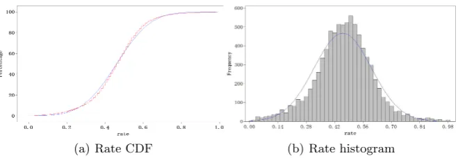
At present, it is extremely hard for citizens to hail a taxi especially on the occa-sion of congested traffic. However, at the same time, taxi occupancy is still very low even in busy time[11]. This contradictory phenomenon leads to great require-ments for customers vehicle transportation. Consequently, there are companies such as Uber[1] which provides private car services to satisfy the above demands. In this manner, private cars become a supplementary to the current taxi service in which citizens could reserve a private car through mobile applications in any place at any time. However, taxicab is inefficient due to characteristics such as low capacity utilization, high fuel costs, heavily congested traffic, and a low ra-tio(live index) oflive miles (miles with a fare) tocruising miles(miles without a fare)[2]. The same challenges exist in private car service as illustrated in Figure 1. The rate represents the ratio of live miles to total miles. Apparently, the rate of approximately 80% vehicles is no more than 0.6. The average rate is merely 0.4601, indicating a typical low live index among most private cars. Namely, idle cruising miles take a large portion of the total miles.
Despite some similar challenges within the taxi service and private car ser-vice, the differences and the root causes still need to be deeply investigated. As for the taxi service, drivers can pick up a passenger easily in rush hours. However, drivers might cruise several street blocks to pick up a passenger if they lack the experience of when and where the citizens usually expect to catch a taxi. There-fore, experienced taxi drivers have less cruising miles than the inexperienced[4]. To mitigate the empirical impacts, many solutions generate and leverage knowl-edge of experience by using historical GPS records, and recommend pick-up positions or cruising routes to drivers for the sake of reducing cruising miles [2][3][9]. However, unlike the taxi service, passengers reserve the cars by Apps in private car service. In fact, each passenger order includes sufficient information such as the current position, destination, appointment pickup time, car type and etc. Intuitively, the abundant information could provision sufficient space to dispatch and schedule private vehicles based on the knowledge mining, giv-ing rise to significant optimization potentials. Without fully utilizgiv-ing of these information, larger cruising miles and longer waiting time will be produced and will result in increasing operating costs and negative user experience. All these strongly motivate our proposal in this paper.
(a) Rate CDF (b) Rate histogram
Fig. 1.rate of live miles compared to total miles
with the following challenges appropriately: 1) predicting the time-varied and dynamic passenger demand accurately; 2) dispatching vehicles to satisfy the re-quirements of different passengers who are free to choose different type of cars; 3) scheduling in real-time manner and provisioning current orders as well as future orders. In particular, the major contributions of the work in this paper can be summarized as follows:
– We propose an innovative study to reduce private vehicle cruising miles and a scheduling method based on a passenger demand model.
– A demand specification model is advocated based on Locally Weighted Lin-ear Regression, which could reach 74% accuracy at most.
– The real-time scheduling is formalized as a weighted bipartite graph match-ing problem and 22.5% cruismatch-ing miles could be reduced by usmatch-ing the described scheduling method.
The rest of this paper is organized as follows. Section2 describes the pas-senger demand model. Section 3 introduces algorithms to dispatch private cars. Furthermore, we evaluate the model and dispatching algorithms on a real dataset in Section 4. Section 5 concludes this paper and discusses the future works.
2
Demand Model
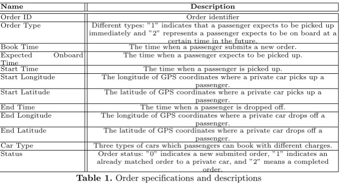
In this section, we elaborate the Passenger Demand Model in detail. Firstly, the training set, formulas and algorithms are respectively described to expose the model’s details. We also demonstrate how to predict the passenger demand in real time manner. To begin with, We make some definitions in terms of the pasenger demand in different contexts. In taxi service, passenger demand mainly indicates the citizen requirements to take a taxi; In comparison, we define passenger’s demand in the private car service as the orders that preserve private cars in a region over a time slot. As Table 1 shows, an order mainly contains such information.
Name Description
Order ID Order identifier
Order Type Different types: ”1” indicates that a passenger expects to be picked up immediately and ”2” represents a passenger expects to be on board at a
certain time in the future.
Book Time The time when a passenger submits a new order. Expected Onboard
Time
The time when a passenger expects to be picked up. Start Time The time when a passenger is picked up.
Start Longitude The longitude of GPS coordinates where a private car picks up a passenger.
Start Latitude The latitude of GPS coordinates where a private car picks up a passenger.
End Time The time when a passenger is dropped off.
End Longitude The longitude of GPS coordinates where a private car drops off a passenger.
End Latitude The latitude of GPS coordinates where a private car drops off a passenger.
Car Type Three types of cars which passengers can book with different charges. Status Order status: ”0” indicates a new submited order, ”1” indicates an
[image:5.595.136.482.114.300.2]already matched order to a private car, and ”2” means a completed order.
Table 1.Order specifications and descriptions
A convex polygon is used to indicate a region space coverage. After statistical analyzing of historical orders, one day could be divided into T time slots and
j(1 <= j <= T) represents the j-th time slot. In addition, each time slot’s duration is regarded as an hour for the sake of understandability, and most works adopt this dividing method[6]. Therefore, the passenger demand in the i-th region over the j-th time slot could be expressed asPi,j(1<=i <=R,1<=j <=T).
Furthermore, based on the mobility of cars and passengers, we assume that passenger demand in one region in the next time slot is relevant to orders in all regions over current time slots. In section 4, we conduct some experiments on a real dataset to confirm these assumptions. In particular, the orders in each region over the current time slot is an argument while the passenger demand in one region in future time slot is independent variable. A set of coefficients can be used to estimate the relation between the orders in current time slot and the predicted orders in the future time slot. To this end, the linear regression model targets our demand and the core philosophy is the coefficients estimation. With the input data stored in matrixX, and regression coefficients stored in vector
w, predicted result can by depicted as Equation 1.
Y =XT·w (1)
To achieve an ideal prediction, the error margin between the real demand and predicted one is supposed to be miminized as possible. The model is utilized to obtain the optimal set of regression coefficients w, given a training set X and
Y. Typically, we aim to find the vector w with the minimum error. In order to improve the computation accuracy, we use the squared error instead of the accumulated errorto represent the required difference. More specifically, the sum of the squared errors(SSE) can be described by Equation 2. The utilized least squares approach find the optimalwwith the least SSE.
SSE=
m
X
i=1
We also depict the SSE in matrix form, as shown in Equation 3 shows.
SSE= (Y −X·w)T(Y −X·w) (3)
We solve SSE’s derivative, and make it equal to zero (Equation 4).
XT(Y −X·w) = 0 (4)
The best regression coefficientswcould be found by using Equation 5.
ˆ
w= (XT·X)−1·XT·Y (5)
It is the best estimation we could achieve from w. It is also worth noting that the above formula contains the requirement for the matrix inversion. Therefore, the equation only works on the occasion of the inversion of matrixXT·X exists.
Typically, the linear regression using the proposed least squares method could obtain the ideal result. However, it might be very likely to encounter with the under-fitting phenomenon. This is because it tries to get unbiased estimation of minimum mean square error and obviously we cannot get the best infer result once the model is under-fitting.
To handle with this problem, we introduce the Locally Weighted Linear Re-gression(LWLR) to produce some bias in the estimation to reduce the mean square error of prediction. In LWLR, we assign certain weights to the sample points which are close to the predicted sample point. In this context, the closest sample point gets the biggest weight. If the weight of a sample point exceeds a certain threshold, it will be selected. Afterwards, the selected points will consti-tute a sample subset. We use least square method to learn the linear regression model on this subset.
We can use the following Equation to get the optimal regression coefficient:
ˆ
w= (XT·W·X)−1·XT·W·Y (6)
W is a weight matrix with each element indicating every sample point’s weight. In order to generate the weighted matrix W, LWLR uses the kernel function to ensure the fact that the sample point closest to the predicted sample point could get the maximum weight. Specifically, there are a number of types of kernel function and the most commonly-used Gaussian Kernel Function is chosen in our solution, as demonstrated in 7.
W(i, i) =exp(|xi−x|
−2k2 ) (7)
In this way, we can build a weight matrixW, containing only diagonal element and the sample point xi closer toxcould finally get the greater weight.
Addi-tionally, k is a user-specified parameter, which determines the weight given to
xi.
Algorithm 1predictPassengerDemandInDifferentRegions() 1: initialize training setX MatrixxM at;
2: initialize training setY MatrixyM at; 3: initialize test setX Matrix X;
4: for allRegion∈Rdo
5: add p(i,j) to X ;
6: end for
7: create weights matrixW;
8: xT x←xM at·T ranspose∗(W∗xM at);
9: if determinant ofxT xequals to 0then
10: returnN U LL; 11: else
12: ws←xT x·Inverse∗(xM at·T ranspose∗(W∗yM at))
13: returnX∗ws;
14: end if
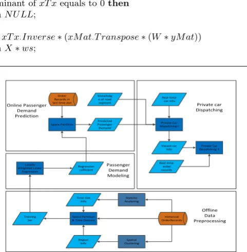
Historical OrderRecords Offline Data Preprocessing Space Partition & Time Division
Region Info Passenger Demand Modeling Locally Weighted Linear Regression Regression cofficient Online Passenger Demand Prediction Order Records in last time slot
[image:7.595.185.426.222.468.2]Space Partition Real-time car info Spatial Clustering Statistic Analyzing Time Slot Info Training Set Predicted Passenger Demand Knowledg e of road segment Real-time order records Private Car Dispatching I Vacant car Info Private Car Dispatching II Private car Dispatching
Fig. 2.Dispatching process overview
description. Secondly, we use the kernel method as described in Equation 7 to generate weight matrix. Finally, after examining if xT xhas an inverse matrix, we obtain the coefficients using Equation 6 and predict the passenger demand in different regions. If xT x does not have an inverse matrix, we cannot figure out the coefficients and the passenger demand. In such conditions, parameter estimation and optimization algorithms are used to facilitate the computation of the approximately optimal coefficients. Due to the fact that xT x’s inverse matrix could be easily obtained in most cases, the parameter estimation is out of the scope of this paper and will not be discussed.
3
Dispatching Algorithm
demand count in different regions could be generated. Before introducing our so-lution, some fundamental definitions are given as follows:
Definition 1 Bipartite graph matching. Given a bipartite graph G = (C,O,E),
C is a vertex set in which each vertex represents a vacant car and each vertex in set O represents a predicted order. M is a subgraph of G. Any two edges in M’s edge set E are not attached to the same vertex and M is a match of vacant cars and predicted orders.
Definition 2 Road Segment. If a road meets a junction or the road offset
ex-ceeds a threshold, a new road segment is generated. A road segment could be uniquely identified by the combination of ID, start and end GPS coordinates.
Assuming that we have estimated passenger demand ˆP(i, j+ 1) iniregion over (j+ 1) time slot. What we need is to assign vacant cars to passengers with the minimum total cruising mileage. A bipartite graph modelG(C, O, E) is therefore used to formalize our problem. Intuitively, distance between a vacant car and a predicted order becomes the weight of an edge connecting those two kinds of vertices. Accordingly, a matching with the minimum weight could be formalized as weighted bipartite graph matching problem.
Before performing the matching algorithm, how to represent the weight of the edges needs to be determined properly. Because the objectives are to find a scheduling method with the minimum cruising mileage, The distance between vacant cars and predicted orders could be used to represent the weights of the edges. In addition,Cis the set of current vacant cars, with a vectorSrecording real-time status of all vehicles. Therefore, we can always get an updatedC from
S. In particular, ”1” indicates that the current passenger vehicle is occupied, whereby ”0” represents a vacant status of the current vehicle. Furthermore, in order to calculate the distance, we have to gain the real-time location of the vehicle. To deal with this, GPS coordinates are adopted to display the car’s position. L represents real-time location information of all vehicles. In this way, we can get current status of the car k fromSk and current position fromLk.
segment. Eventually, the position of the predicted order can be determined by this road segment.
Moreover, we will discuss how to set the weight of edge. In bipartite graph G (C, O, E), E is the set of edges. Intuitively, the distance between the car and the order is used to represent the weight of edge between them. Despite other factors including the weather, real-time traffic etc, we use Baidu Web APIs to get the shortest distance between two GPS coordinates in our experiment for the clearness and simplicity of the model.
Given above definitions and descriptions, the scheduling problem could be formalize as a weighted bipartite graph matching problem. Kuhn-Munkras al-gorithm is used to find the optimal matching with minimum cost. Due to the special nature of KM algorithm, set C and O should have equal vertexes. In fact, we can add some vertexes to the minimum set on the occasion of two unequal set. Additionally, the weights of edges associated to those added vertexes are set to be zero. The detailed descriptions of the scheduling process could be found in Algorithm 2 .
Algorithm 2schedulePrivateCar()
1: initialize each vertex in set C in j+1 time slot; 2: predictPassengerDemandInDifferentRegions (); 3: initialize each vertex in set O in j+1 time slot; 4: find a minimum cruising mileage matching;
5: whilea real order occursdo
6: select vacant cars near the real order’s position ; 7: if a vacant car accepts the orderthen
8: update car’s status; 9: update order’s status; 10: update L and S;
11: end if
12: end while
After the matching decision, vacant cars will be assigned to the road segments where predicted order exists.
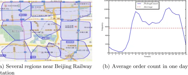
(a) Several regions near Beijing Railway Station
0 1 2 3 4 5 6 7 8 9 10 11 12 13 14 15 16 17 18 19 20 21 22 23 Time(h)
0 200 400 600 800 1000 1200
Frequency
PickupCount Average
[image:10.595.142.456.132.258.2](b) Average order count in one day
Fig. 3.Regions and time slots
4
Experimental Evaluation
In this section, we set up several experiments to evaluate the effectiveness of the proposed passenger demand model and dispatching algorithm.
4.1 Dataset and Experiment Environment
We use a real dataset from a private car hiring company (for commercial reasons we cannot identify the name), which contains 2720 vehicles and 356706 order records for a whole month in Beijing. The test machine is equipped with De-bian 6.0 operation system, 8GB Memory and Intel i5-4570 with a frequency of 3.20GHZ is set up.
4.2 Data Processing
Because the real dataset can not be directly used, the data processing starts with data cleaning and pre-operations. Specifically, we filter the order with a time duration less than 10 minutes and larger than 60 minutes, resulting in the remaining 324512 records. Subsequently, spatial clustering is utilized to split Beijing urban area into multiple regions. To simplify our experiment, DBSCAN algorithm is used to divide urban areas in Beijing four-rings into 136 areas. Two parameters (Epsilon and MinPoints) are set to be 0.15 and 100 respectively according to the engineering experiences. Actually, the Epsilon indicates the density of a region , while MinPoints shows how many points a region need to possess at least. Besides, a day is partitioned into several time slots based on the order distribution in one day.
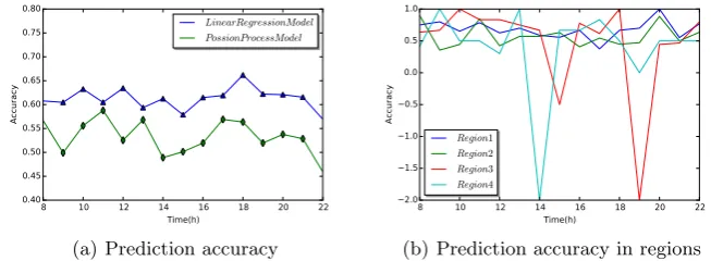
8 10 12 14 16 18 20 22 Time(h)
0.40 0.45 0.50 0.55 0.60 0.65 0.70 0.75 0.80
Accuracy
LinearRegressionModel PossionProcessModel
(a) Prediction accuracy
8 10 12 14 16 18 20 22 Time(h)
2.0 1.5 1.0 0.5 0.0 0.5 1.0
Accuracy
Region1 Region2 Region3 Region4
[image:11.595.139.466.129.249.2](b) Prediction accuracy in regions
Fig. 4.Passenger Demand Model Evaluation
4.3 Model Evaluation
We firstly introduce Non-homogeneous Poisson Process (NHPP) Model. Poisson process is a stochastic process that is often used to study the occurrence of events. It assumes that the arriving rate of events λis constantly stable, and has the Poisson distribution of counting and exponential distribution of inter-event time. In fact, NHPP[8] is a specific Poisson process with a time-dependent arriving rate functionλ(t). The model is more flexible and appropriate to depict the human-related activities because these activities often vary over time but have strong periodicity. We use ∆T to indicate time increment and N(∆T) to represent order increment in ∆T. Specifically, N(∆T +j)−N(j) follows the Poisson distribution with a parameter λ∆T.
P{N(λT +j)−N(j) =k}=e
−λ∆T(λ∆T)k
k! (8)
Here we set ∆T to one hour and λ can be obtained by maximum likelihood estimation:
ˆ
λ= N
∆T (9)
where N can be denoted by average orders in one hour. Therefore, we could use the average order count to predict passenger demand. We use the following equation to calculate the prediction accuracy:
Accuracy= Pi,j+1− |Pi,j+1−Pˆi,j+1|
Pi,j+1
(10)
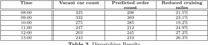
Time Vacant car count Predicted order count
Reduced cruising miles
08:00 325 296 21.5%
09:00 332 369 23.1%
10:00 275 285 19.2%
11:00 247 212 24.9%
12:00 203 245 27.2%
[image:12.595.134.481.116.191.2]13:00 243 210 26.3%
Table 2.Dispatching Results
reveals the prediction accuracy of different regions. Apparently, the accuracy for Region 1 and 2 is steady all the time with little fluctuation. However, the infer-ence accuracy in Region 3 and 4 suffers from some degrees of variations, even with some outlier results. This is because the number of orders in these Regions are so scarce that the proposed model could not capture a reasonable value. To solve this problem, we not only enlarge the size of required dataset, but increase the region’s coverage area as well.
4.4 Dispatching Algorithm Evaluation
In order to replay the real behaviors of the moving vehicles and the user demands, we emulate their moving traces obtained from the historical data and apply them into our algorithms. As shown in Table 2, we choose the real orders and car traces from 08:00 to 13:00 on May 6th,2015. At 8:00, there are 324 vacant cars and 296 predicted orders in this evaluation. The results illustrates that the proposed model could finish matching of vacant cars with predicted orders in 52 seconds. In addition, we leverage Baidu Web API to obtain the distance between a vacant car and a predicted order with average speed recorded. Once a real order emerges, the nearest vacant car could be selected to pick up the passenger. On average, 22.5% cruising miles could be reduced in this simulated experiment.
5
Conclusions and Future Work
dataset to optimize the proposed model and to take more factors into consider-ation which affect passengers demand, such as weather, holidays etc. Moreover, we are also planning to parallelize the dispatching algorithm to further reduce the total execution time.
Acknowledgments This work is supported by grants from the National
Nat-ural Science Foundation of China (No. 91118008).
References
1. Uber,https://www.uber.com
2. Powell, J. W., Huang, Y., Bastani, F., & Ji, M. Towards reducing taxicab cruising time using spatio-temporal profitability maps.. Lecture Notes in Computer Science, 6849, 242-260 (2011)
3. Qu, M., Zhu, H., Liu, J., Liu, G., & Xiong, H. A cost-effective recommender system for taxi drivers. Proceedings of the 20th ACM SIGKDD international conference on Knowledge discovery and data mining. ACM. (2014)
4. Yuan, Jing, et al. ”Where to find my next passenger..” Proceedings of the 13th international conference on Ubiquitous computingACM, 2011:109-118. (2011) 5. Huang Y, Powell J W. Detecting regions of disequilibrium in taxi services under
uncertainty[J]. Proceedings of International Conference on Advances in Geographic Information Systems, 2012:139-148. (2012)
6. Zhang, D., He, T., Lin, S., Munir, S., & Stankovic, J. A. Dmodel: Online Taxicab Demand Model from Big Sensor Data in a Roving Sensor Network. Big Data (Big-Data Congress), 2014 IEEE International Congress on(pp.152-159). IEEE. (2014) 7. Zhang, Desheng, and T. He. ”pCruise: Reducing Cruising Miles for Taxicab
Net-works.” 2013 IEEE 34th Real-Time Systems SymposiumIEEE, 2012:85-94. 8. Zheng, X., Liang, X., & Xu, K. Where to wait for a taxi?. Proceedings of the ACM
SIGKDD International Workshop on Urban Computing. ACM. (2012)
9. Yuan, N. J., Zheng, Y., Zhang, L., & Xie, X. T-finder: a recommender system for finding passengers and vacant taxis. IEEE Transactions on Knowledge & Data Engineering, 25(10), 2390-2403. (2013)
10. Ester, Martin, et al. ”A Density-Based Algorithm for Discovering Clusters in Large Spatial Databases with Noise..” Proceedings of International Conference on Knowl-edge Discovery & Data Mining(1996):226-231.
11. Chang, H. W., Tai, Y. C., & Hsu, Y. J. Context-aware taxi demand hotspots prediction.. International Journal of Business Intelligence & Data Mining, 5(1), 3-18. (2010)
12. Kiam Tian Seow Nam Hai Dang Der-Horng Lee. A Collaborative Multiagent Taxi-Dispatch System[J]. Automation Science & Engineering IEEE Transactions on, 2010, 7(3):607 - 616 (2010)
13. Ge, Y., Xiong, H., Tuzhilin, A., Xiao, K., Gruteser, M., & Pazzani, M. An energy-efficient mobile recommender system. In Proc. KDD 2010(pp.899–908) (2010) 14. Li, Bin, et al. ”Hunting or waiting? Discovering passenger-finding strategies from