DYNAMICAL SYSTEMS FOR
LEARNING AND
BALANCING
Jane Elizabeth Perkins
BSc
(Hons)
,
University of Western Australia
May
1992
A thesis submitted for
the
degree of Doctor of Philosophy
of the A ustralian National University
Department of Systems Engineering
Declaration
The contents of this thesis are the results of original research, and have not been submitted for a higher degree at any other university or institution. These doctoral studies were conducted with Professor John B. Moore as supervisor. The extent to which the research herein is my own work, not reliant on Professor Moore and my other colleagues, is outlined in the Preface.
A number of papers resulting from this work have been submitted to refereed journals:
[JI] J .E. PERKINS, U. HELMKE, J .B. MOORE, Balanced realizations via gra-dient flows, Systems and Control Letters 14 (1990), 369-377.
[J2] J.E. PERKINS, I.M.Y. MAREELS, J.B. MOORE A D R.W. HOROWITZ, Functional Learning in Signal Processing via Least Squares, Signal
Process-ing and Adaptive Control, to appear.
[J3] J. IMAE, J .E. PERKINS, J .B. MOORE, Towards time varying balanced realization via Riccati equations, Mathematics of Control, Signals and Sys-tems, to appear.
[J4] U. HELMKE, J .E. PERKINS, J .B. MOORE, Finding Balanced Realizations using Differential Equations, SIAM Journal on Control and Optimization, to appear.
[J5] B.D.O. ANDERSON, G. LI, M. GEVERS, J .E. PERKINS, Optimal FWL Design of State-Space Digital Systems with Weighted Sensitivity Minimiza-tion and Sparseness Consideration, IEEE Trans. Circuits and Systems, to
A number of papers have been presented at conferences. Some of the material presented in these papers overlaps with that covered in the publications listed above:
[ell
J.E. PERKINS, U. HELMKE AND J.B. MOORE, Differential Equations for Singular Value Decomposition, 1991 Conference on Decision and Control.[C2]
J.E. PERKINS, I.M.Y. MAREELS, J.B. MOORE A D R.W. HOROWITZ,Functional Learning in Signal Processing via Least Squares, International Symposium on Information Theory and its Applications, Hawaii 1990.
Preface
The work described in this thesis has been carried out in collaboration with a number of people. When working in a group at a white board, or over a cup of coffee, it is impossible to say exactly who contributed what. The parts I particularly identify with are summarized as follows .
• In Chapter 2, my role has been combining the ideas of different people, along with my own contributions, into one coherent algorithm. In particular recognising the similarity between the "spread function" and "interpolation function", that are now combined. This algorithm evolved over a series of meetings, and was subject to many reconstructions. I produced the computer simulation results, and experimented with different interpolating
functions .
• For the work in Chapter 3, I produced computer simulations that have been useful in demonstrating the unique convergence, as well as revealing the ex-ponential rates of convergence, both of which were subsequently established theoretically. I have contributed to the uniqueness proofs, and the proofs of exponential convergence rates. Generally my role has been to transform the ideas of my supervisor into working algorithms, with useful properties .
• In Chapter 4, I developed the exponential convergence rates, the computer simulations and the final proof for the diagonal algorithms, as well as in-teracting in the discussions about the other results .
solutions were developed by Joe Imae. The original proofs were awkward, and I reworked the results gi ving global convergence and a bound on the error. A third proof version was the result of a meeting between Uwe Helmke and myself. For interest, the intermediate proof is included in Chapter 5 of this thesis, and the newest proof method is used for similar results in Chapter 6 .
Acknowledgements
John's supervision and "philosophy of research/life" talks have been invaluable. The student supervisor relationship is very special, and its proper functioning is vital for fruitful interaction, learning and research. I thank John, and his wife Jan, for their care and friend hip over the last three years.
The Systems Engineering department has given me the chance to interact with
people from diverse backgrounds. Those I have worked with have been interesting and I thank them for their encouragement. The courses I have taken whilst undertaking my PhD have given breadth of learning, not to mention some nice proof tricks for my research. I wish to congratulate those lecturers responsible. Particular mention must go to those, both visitors and staff, that I had the pleasure of researching with - Uwe Helmke, Iven Mareels, Joe Imae, Roberto Horowitz. Students have also played an important role in making this a dynamic environment, thank you.
To my fellow students from Perth - thank you for providing encouragement at the low points, a steadying influence at the high points, and warm friendship throughout our PhD studies.
Australia Post and Telecom have proved up to the task of keeping me near those who mean so much to me (the airlines failed occasionally). Without their long distance support my quality of life would have been poorer.
Abstract
In this Thesis methods of exploiting new computer technology in the area of system identification are investigated. In particular computing methods that can take advantage of parallel processing are explored.
The results in this thesis can be implemented to allow the learning of a non-linear function, or the solution of a balancing task, with the answer becoming more accurate as time evolves. Both of these tasks are presented in a way that can be readily extended to a time varying setting. The dynamic nature of the algorithms are also useful in the area of system uncertainty.
The first part of this th~sis extends known Kalman filter algorithms to the multidimensional case. Representation theorems show that a function can be represented as the sum of other known functions. The aim is then to learn an unknown nonlinear function, possibly in a noisy environment, as the sum of other known functions. Kalman filters are used to estimate the coefficients of the function summation. Such a bank of Kalman filters is readily adapted to parallel processing, but this is not done here.
Table of Notation
The following is a summary of some of the notational conventions to hold through-out this thesis. There are a few instances of repetition, due to a desire to use
notation standard to each field of research. Thus, the notation appearing in the "Functional Learning" section below is specific to Chapter 2, and the notation appearing in the "Differential Equation" section below holds throughout the
re-mainder.
Mathematical
IR the set of real numbers N the set of natural numbers In the unit cube in IRn
A' the transpose of A
D
a diagonal matrixdiag( d1 , .. . , dn ) the diagonal matrix with diagonal entries d1 , ... , dn D~(x)( derivative of ~ at
x
in the direction (GL(n, IR) set of real invertible matrices of rank n
tr the trace of a matrix, i.e. the sum of the diagonal elements
Ai
an eigenvalueAm.in minimum eigenvalue Amax maximum eigenvalue O(k) order k
[image:9.620.22.602.17.757.2]TM T*M
\\AII
( , ) [A,B] a.s.a, Ti, E, (3, C
Ti
fU
j
j(x,
Q)
,i
Ki(X)
KIKB(X)
Pk <Pk <PIQ
Q*
the tangent space at a point x in a smooth manifold M the tangent bundle of a smooth manifold M
the cotangent bundle of a smooth manifold M
the norm of A, (if there are several norms used, this is specified) inner product
Lie bracket, AB - BA
Functional Learning
almost surely constants
mean square integral error measure mean square discrete error
upper bound of persistence of excitation
lower bound of persistence of excitation function to be learnt
estimate of
f
estimate of
f(
x) given coefficient estimates·Q a point in spacethe set of interpolating points input variable space
point in fI
interpolating function
vector of interpolating functions vector of basis function evaluation at x error covariance
regression vector of past Yk, Uk
coefficient of the ith basis function vector of
qi
Q*
optimal estimate of Q0"( t)
sigmoid functionO"b
(t)
bisigmoid functionI) parameter vector to be learnt
8(Xk) function of Xk to be learnt I)k estimate of I) at time k Wk nOIse sequence
Wk weighting matrix at time k
Xk inputs
Yk outputs
Differential Equations
A the time derivative of A \l A the gradient of A
(A,
B,
C) a system realizationAlp the function A evaluated at P G( s) a transfer function
11 the gain of the differential equation for time varying balancing P(n) set of symmetric positive definite matrices of rank n
<I>, r/>,
e
,
Ill,:=:
cost functions<I>(A,
t)
Ra
X
the transition matrix for the homogeneous system the set of all realizations of a given transfer function
Contents
Declaration
Preface
Acknowledgements
Abstract
Table of Notation
1 Introduction
2 Functional Learning
2.1 Introduction .. .
2.2 Preliminary Definitions and Theorems 2.2.1 Function Representation ..
111
v
VI
V111
1
6
6
9
10
2.2.2 Least Squares Convergence. 11
2.3 Least Squares via Basis Functions (one dimensional problem) 13 2.3.1 The Signal Model. . . . . . . . . . . . 13 2.3.2 Measures of Error and Minimization Task 14 2.3.3 Allowable Basis Functions and Reconstructibility
2.3.4 Recursive Least Squares Algorithm
2.4 Interpolation Functions in Least Squares 2.4.1 Signal Model . . ,
2.4.2 Reconstructibility.
2.4.3 Allowable Interpolation Functions
15 17
19
19
19
[image:12.620.48.604.16.756.2]2.4.4 Least Squares Algorithm
2.5 umerical Simulation . 2.6 Conclusion . . . .
3 Linear Algebra and Differential Equations
3.1 The Link - History and Motivation
3.2 Gradient Flows . . . .
3.2.1 Riemannian fetrics and Gradient Flows 3.3 Linear Algebra Tasks to be Considered
3.4 Summary of Useful Matrix Properties. 3.5 Balanced Matrix Factorization .
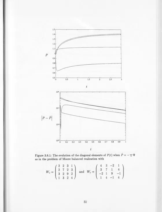
3.6 Balanced Realization 3.7 Norm Minimization. 3.8 Convergence Properties. 3.9 Conclusion . . . .
4 Gradient Flow to find Balanced Realizations
4.1 Introduction . . . .
4.2 Gradient Flows for Balancing Transformations
4.2.1 Balancing Flows of Positive Definite Matrices
4.2.2 Gradient Flows for Balancing Transformations
4.2.3 Diagonal Balancing Transformations ..
4.3 Differential Equations on the System Matrices. 4.4 Application to SVD .
4.5 Conclusions . . . . .
5 Time Varying Balanced Realization
5.1 Introduction . . . 5.2 System description and assumption
5.3 Time Varying Case 5.4 Simulations
5.5 Conclusion.
6 Time Varying Balanced Factorization
6.1 Introduction .. . . . 6.2 Time-Varying Differential Equations on P
6.2.1 Strengthened Time-invariant Theory
6.3
6.4
6.5
6.2.2 Time-Varying Differential Equations on P
Gradient Flow on onsingular Matrices T
Flows on the Factors X and Y .
Conclusion .
7 Conclusions
97
97
99
103
104
107
110
115
Chapter
1
Introduction
eural etworks are currently seen to hold promise for implementing artificial
intelligence systems. Their evolution, together with technological advances are
changing the type of computing methods we use. Parallel processing suggests we
should organize large problems into a set of small tasks that can be performed in
parallel. eural networks have opened the possibility of reintroducing the analog
computational approach. Computer memory and the computational power of our
desk-top computers is increasing, thus allowing us to study new computational
methods. These factors all suggest a need to look at how we can do our
compu-tations to take advantage of these new parallel technologies as they emerge. This
thesis investigates methods of using this computer technology in learning about
a plant, balancing the controllability and observability properties of a plant, and
the related tasks of matrix factorization such as the singular value decomposition.
An area of particular research interest in this thesis is that of dynamical
sys-tem identification, that is finding a set of iteritive mathematical equations that
describe a physical system. This is an important preliminary or concurrent
oper-ation to engineering any estimation, prediction, or control strategy for controlling
the system. Clearly the accuracy of any system identification will determine the
performance of any estimator or controller based on this identification. In the
engineering context, on-line identification is important so that as each new
consequently of the controller, with minimal delay. Much of the identification literature is in the area of linear systems theory. However the question of non-linear system identification is important since clearly many physical systems are nonlinear.
A possible approach to nonlinear system identification is via functional learn-ing, that is finding a functional representation for the underlying nonlinearities of a system. A number of the results in neural networks can be applied for functional learning of nonlinearities in a dynamical system. Such algorithms converge very slowly, and certainly the convergence theory is incomplete. As an alternative ap-proach, it seems reasonable to try to extend known identification algorithms, with well understood convergence properties, to the functional learning setting, rather than develop convergence results in the neural network setting where the theoret-ical issues appear too formidable at this stage. As a starting point in our research it is proposed that familiar least squares techniques be used to learn functional representations of parameters of an ARMAX system, with convergence results given in terms of persistence of excitation conditions over the function space, as well as in time. A key feature of the approach is that it, in common with the neural network approach, is amenable to parallel computer processing.
An identification algorithm will often result in a system model with a high complexity. For engineering applications the model must have a low enough com-plexity to readily allow rapid calculation and low hardware complexity, increasing reliability. Model order reduction is a process whereby we can reduce the
com-plexity of the model with minimum reduction of modelling accuracy. A standard approach to this task for linear systems is via a technique called balanced real-izations, which organizes the state space representation of a system so that each internal variable (state) is equally controllable from the input and observable from the output. Traditionally this task is achieved by performing algebraic matrix
manipulations. The methods explored in this thesis concern finding the balanced realization as the limiting solution of a system of differential equations which can be updated, in principle, via an analog computer (or parallel) approach.
opening the way to dealing with realizations functionally dependent on the
sys-tem state. Balanced realization itself can be viewed as a learning problem: Given
a starting realization, how do we modify our system representation in order to
minimize the difference between the observability and controllability gramians.
The learning nature is more obvious when the differential equations can be
inter-preted as a gradient descent or flow in which case there is an obvious minimization
objective.
onlinear systems can be locally approximated by a linear system. In this
way a nonlinear system can be viewed as a time-varying system. Systems that are
still being learnt can also be viewed as time-varying systems. In these cases, as
well as genuine linear, time-varying systems, it is desirable to find a time-varying
balanced realization. The differential equation approach allows such a realization
to be found to arbitrary accuracy.
A differential equation approach can also give new insight into the solution
of other balancing type tasks. As these techniques become available tasks like
minimum sensitivity of a closed loop can exploit these insights.
Chapter 2 addresses certain functional learning tasks in signal processing using
familiar algorithms and analytical tools of least squares for autoregressive moving
average exogenous input (ARMAX) models. The models can be viewed as
con-ventional ARMAX models but with parameters dependent on variables such as
inputs or states, termed function input variables. The functional dependence of
the parameters on these variables is represented in terms of basis function
expan-sions, or more generally interpolation function representations. The interpolation
functions in a least squares identification of coefficients also turn out to be, in
essence, spread functions that spread learning throughout the space of function
input variables. Thus for a set of training sequences, or trajectories in function
input space, system parameters and thereby system functionals can be updated.
The idea is that these will have relevance for similar sequences or neighbouring
trajectories. The concept of persistence of excitation to achieve complete function
learning, or equivalently, signal model learning is studied using least squares
signal processing context is addressed by means of simple illustrative examples. In Chapter 3, the link between differential equations and linear algebra is explored. These ideas are developed in subsequent chapters, but background material is given here. Three balancing tasks, namely balanced factorization, balanced realization, and a new type called norm minimization, are shown to be equivalent to finding limiting solutions of certain gradient flow differential equations. By viewing such algebraic tasks in the context of calculus, they are amenable to analog computational solutions, or parallel processing machines, perhaps even neural networks. The convergence rates of the differential equations are exponential, and consequentially convergence is rapid and numerical stability properties are attractive.
In Chapter 4 the task of finding balanced realizations in systems theory using differential equations is investigated in further detail. Several alternative sets of equations, giving both diagonal and generalized balancing, are given, evolving on both transformation matrices and the system matrices themselves. The flows that evolve on the actual system matrices remove the need for considering coordinate transformation matrices. Convergence properties are examined in this chapter.
Chapter 5 explores the ability of the Riccati equation to solve the balanced re-alization task. This approach is then extended for solving time-varying balanced realization problems. Instead of calculating the exact solutions for balancing at each time instant, we estimate with arbitrary accuracy the balancing solutions by means of the Riccati differential equations associated with the balancing prob-lems. Under uniform boundedness conditions on the controllability gramians and their inverses, the solutions of the Riccati equations exist and converge exponen-tiallyas their initial time goes to - 0 0 to give what we term l1--ba/ancing solutions. The parameter 11- has the interpretation of the gain of a differential equation. It determines the accuracy of the balancing transformation tracking and the expo-nential rate of convergence. Their exponentially convergent behaviour ensures numerical robustness.
flows proposed in earlier chapters to solve time-invariant balancing tasks. Differ-ential equations are proposed that evolve on the relevant transformation matrix, its square, or the matrix factors. The solution to time-invariant problems is achieved exponentially, and that of the time-varying problem is achieved with a "tracking" error which can be made arbitrarily small.
Chapter 2
Functional Learning
2.1
Introduction
The current neural network literature has highlighted the task of functional
learn-ing for application within the fields of control systems, and signal processing. The
idea is that some input-output function
f(·
)
is learned by means of a trainingse-quence of function inputs Xk and outputs Yk for k
=
1,2, ... , r asj(-).
Thefunction estimate
j(-)
can then be used to achieve outputs Y from inputs x asY =
j(x
).
Of course, neural networks are usually restricted to the set of
parametriza-tions for
j(-)
in terms of suitably parametrized sigmoid functions and weights in amulti-layer network. The parameters and weights are learnt by various methods
including backward propagation and extended Kalman filters [30]. The
repre-sentations are such that the functions are not linear in the parameters/weights
so that standard least squares, or weighted least squares, parameter estimations
techniques do not apply.
For a number of reasons it would be of interest to pursue the role of least
squares techniques for functional learning where the functions are linear in the
parameters (weights). Least squares methods can be truly recursive in that
esti-mates can be updated as each new measurement arrives. Also, they are readily
the adaptive control and signal processmg context where they are ubiquitous.
It has been a natural development for such adaptive methods to evolve towards learning systems where the underlying task is functional learning rather than pa-rameter estimation. Thus in the trivial functional learning environment, when the function is linear and constant, it is appealing for the learning algorithms to specialize to the well-understood least squares based parameter estimation schemes.
A key property of least squares algorithms is that their convergence depends on certain excitation conditions of the regression vectors, which in turn depend on external excitations. This property, in the adaptive estimation context, should carryover to the functional learning context. In earlier studies [20], [15], [22], the concept of functional persistence of excitation is developed for continuous-time deterministic systems in an infinite dimensional setting, working with integral operators. The kernel functions allow information to spread in the function in-put space. Application studies for the control of robots are performed using discrete-time and gradient or least squares ideas. From this work, the question that naturally emerges is: What are fundamental results concerning functional learning and persistence of excitation in a least squares stochastic identification context?
In this chapter we interpret a class of functional learning tasks as least squares parameter estimation tasks, or a system of lower order least squares parameter estimation tasks performed in parallel. One of the main ideas used in the chapter is that in learning a function
f(·)
at a point, from input-output measurementsXk, Yk, the closer Xk is to " the greater the influence of the pair Xk, Yk should be in learning
fh).
Thus for Xk in the neighbourhood of " the associated weightings are high relative to weightings for Xk outside the neighbourhood of ,. The weightings then control what can be termed the spread of learning.The algorithm we propose, in its most general form, seeks function esti-mates, or rather function parametrization estiesti-mates, at a set of points
r [
=strongest in the neighbourhood of Xk and diminished, or even zero, outside this neighbourhood. With estimates at
r [,
an interpolation function can be used to give estimates onr
x . In fact, in our algorithm, the interpolation function is also used to control the spreading out of learning. Because of this dual role for the interpolation function, we must select bisigmoidal functions K;(x) which decay to zero outside the neighbourhood of Ii. Thus polynomial, spline, and Fourier basis or interpolation functions are not an appropriate practical choice although some of our formulations allow such function representations.The second principle idea dealt with in the chapter concerns the convergence of least squares algorithms in the functional learning context. Known conver-gence theory for the least squares algorithm can be applied. Thus in any calcu-lation, convergence behaviour can be estimated on line in terms of persistence of excitation measures on variables used in the calculations, under appropriate as-sumptions. It is, of course, desirable to translate such excitation conditions onto external variables. We claim that the (functional) persistence of excitation con-ditions for consistent estimation of the function, under function reconstructibility conditions, are a natural generalization of the available theory for the parameter estimation context, making connections to related work [22].
So as to generalize least squares based adaptive schemes in signal processing and control, we work with signal models which are natural generalizations of familiar input-output models in these fields.
The aim is to learn the functional representation of the coefficients of the discrete-time "ARMAX" equation, specialized to the white noise case, namely
(2.1.1)
types of least squares algorithms to estimate (possibly matrix or vector) function
representations
f
(x)
of the coefficientsai
(-),
bl).
Of course, (2.1.1) is a special case of the more general form
(2.1.2)
When specialized to (2.1.1), we have 8'(-)
=
[al(-)
'
"
an(-)bl(-) ... bm(-)] and<I>~
=
[Yk-l ... Yk-nUk-l ... Uk-m]. Our objective is to estimate the (vector ormatrix) function 8(·) from knowledge of the sequences Xk, Yk, <I>k.
One example where functional learning in dynamical systems can arise is in
gain scheduling for an aircraft controller, where the function input variables Xk
are the speed and altitude of the aircraft and
f(
Xk) is the gain schedule. Anotherpossible application area is in robotics, [22], where Xk could be the position, and
orientation, of the robot hand in space. In these two cases the parameters of the
linear system are functionally dependent on the position. The optimal control is
then also a function of position. The aim is then to learn the control function,
given calculations at discrete points.
In Section 2.2, some theorems are reviewed concerning functional
representa-tion, and least squares convergence. In Section 2.3, the standard type of least
squares method is applied to functional learning, and in Section 2.4 the idea of
interpolating functions is exploited for this context. Section 2.5 has some
simula-tion results and observations on practical implementation. In Section 2.6, areas
that require further investigation are discussed and concluding remarks made.
2.2
Preliminary Definitions and Theorems
This section on functional representation and least squares convergence can be
2.2.1
Function Representation
For some of the results to follow we focus on representing a function as a sum of
simply parametrized functions, termed here representation functions. Examples of such representation functions are sigmoids, and bisigmoids. The definition of these functions are now recalled.
Definition 2.2.1 A scalar sigmoid function of a scalar variable t is one of the
form
{
I t - t o o
a(t)
=o
t - t - 0 0This general definition does not require continuity, however the sigmoids we are
interested in are piecewise continuous. An example of such a scalar sigmoid
function is
a(t)
= (1+
e-tt 1.Definition 2.2.2 A scalar bisigmoid is the difference of two offset sigmoid
func-tions with the property
Ub(t)
~
u(t)
~
u(t
~
1)
~
{
~
t-t-OO
We are interested in integrable bisigmoids generated by a monotonic sigmoid. The function
ab(t)
= (1+
e-t)-l - (1+
e- t+1 t l is clearly an example of such a scalar bisigmoid.Another function that is of interest is the familiar Gaussian function with covariance
~i,
assumingI~il
f
0, isg(t)
=
(J27rI~il)-1
exp(_t/~ilt/2
)
.
A theorem about functional representations on a compact interval is now re-viewed. This theorem gives conditions for approximating an arbitrary integrable function, to an arbitrary accuracy, using a given error measure. These conditions justify the use of continuous sigmoids and integrable bisigmoids as representation functions.
We use the notation that JR is the set of real numbers and N is the set of natural numbers. Consider
Let us define
r q
I)G)
=
{g: g(x)=
~
(3jG(yjx+
Zj); x, Yj E lRn, q E N, Zj, {3j E lR})=1
Theorem 2.2.1 Denote the unit cube in lRn by
In. If G(-) E £1) the space of absolutely integrable scalar functions) and
h
G(t) dt =I- 0) then Er(G) is dense in£1 (In)
Proof The proof of this can be found in [7].
•
Similar theorems are given in [7],[33] that give conditions for dense function representations over the space of continuous functions. An immediate conse-quence of this theorem is that sums of absolutely integrable bisigmoid functions are dense, in the L1 sense, and can approximate absolutely integrable functions over finite domains.2.2.2
Least Squares Convergence
The theory of least squares gives a method of finding the constant coefficient B
of the equation
(2.2.1)
where
Yk
is an m vector, CPk is an r X m matrix,B
is an r vector, andWk
is an m vector of white Gaussian noise, independent of CPk and B. Here the task is to selectB
as to minimize a weighted square of the error. That is, to minimize with respect to ( the functionVk(O
=~
t(Yi - cp;O'Wi(Yi -
cp~()
,
i=O(2.2.2)
where Wk = W
k
>
0 are the weighting matrices. The optimal ( at time k, denotedfh,
is given from the recursionwhere Pk is an invertible m x m matrix, and with appropriate initial conditions.
Theorem 2.2.2 Consider the weighted least squares algorithm (2.2.3), (2.2.4)
applied to the signal model (2.2.1). Then, as k --t 00, Pk --t Poo , {h --t ()oo
a.s. Consider also that () is a random variable with a normal probability density function
N[()o,
Po],
and that the noise Wk is independent with a probability densityfunction N[O, Wk-1]. Then the conditional distribution of ()k, given Yl ... Yk, has mean {h given by (2.2.3) and covariance Pk given by (2.2·4)· Moreover, if Poo =
°
a.s., then limk~oo {h = () a.s.
Proof The proof of this can be found in
[32].
•
Remarks:
1. Actually, if the regression vector <I>k is not influenced by the estimates
{h,
then the initial condition restriction in the theorem can be relaxed, as indeed can the interpretation of Wk- 1 as a noise covariance. See[32].
2. Convergence rates for {h are according to the convergence rates for Pk.
Precise results on this can be found in
[5]
for the case when () is not requiredto be a random variable. Thus with Wk a martingale increment process with
bounded second moments,
a.s.
(
2.2.5)
where Amin denotes the minimum eigenvalue. Of course, if for all j, and some N,
a.s. (2.2.6)
3. In the noise free case it can be shown that the convergence of {h to () is at
2
.
3
Least Squares via Basis Funct
i
o
ns
(one dimensio
nal p
roblem)
2.3
.
1
The S
i
gnal Model
Here we examine a standard problem in (deterministic) approximation theory, in order to gain insights for the (stochastic) learning problem which is the focus of this chapter. In particular, we work with basis function expansions and em-ploy least squares parameter estimation for estimating the coefficients in a basis function expansion.
Consider for simplicity the square integrable functions
f: fx --t JR,x 1-+ Y
=
f(x)K;:
fx --t JR,x 1-+K;(x)
,
(2.3.1a)
(2.3.1b)
where fx C JR. Let us investigate finite representations estimating f(x) of the form
n
j(x; Q)
=L
K;(x)q;
= K~(x)Q, (2.3.2);=1
where
Here
Kl)
are known square integrable basis functions andQ
is a parameter vector estimate.We observe data points (Xk, Yk) generated as:
2.3
.
2
Measures of Error and Minim
i
zation
T
a
s
k
Consider now in what sense the function representation is required to approximate the function. It is desirable to work with a global measure of the error
f(x)
-j(x; Q),
for allx
Er
x under (2.3.1a), (2.3.2). An example of such a measure is1
d2(Q)
=[fr
r
IIJ(x)
- j(x;Q)
11 2
dx
r
,
(2.3.3)which is the mean square error measure. With
f(xk)
available only at a discrete set of points Xk Er
x, it makes sense to consider a restricted measure of the meansq uare error as
(2.3.4 )
In approximating functions (2.3.1a) by function representations (2.3.2), the min-imization task we focus on is as follows
(2.3.5)
or the closely related index
(2.3.6)
Remarks
l. It is really the error measure d2
(Q)
that is of interest, because this gives ameasure of the error at both the points that have been visited and those for which a function estimate is given. In any application, only measurements at a finite set of points are available, so d~r)(Q) is the only realistic error measure to work with. In the situation that
f(x)
is smooth and the pointsXk are chosen in a uniformly dense way, standard calculus theory tells us that the d~r) error measure approaches the
d2
error measure.2. Another example of an error measure which is appropriate in some
situa-tions is
There is in fact a whole family of possible error measures of the form
which may have merit for particular applications. In the sequel however we are concerned only with the d2 error measure.
3. The error measure only considers the functional representation on the region
r
x. It will be dependent on the application as to whether values should betruncated outside this region or not.
2.3.3
Allowable Basis Functions and Reconstructibility
If one function f(x) is to be represented as a sum of other functions, it is necessary that the possible function summations,
j(x,
Q),
be sufficiently rich to allow a reasonable approximation. Representation theorems like 2.2.2 are important in giving conditions as to which functions can be used in such representations. There are obvious disadvantages if there exist Ql#-
Q2 such thatj(x,
Qd =j(x
,
Q2) for all x Er
x. It is also necessary that. the measurements that are used to choose the function representation are sufficiently rich to characterize the behaviour of the function being approximated. There is a need in some of the theory to follow, for restrictions on the function representations as well as on the class of function that is estimated. Of particular interest are allowable basis function representations and the class of reconstructible functions.Definition 2.3.1 The set of square integrable basis functions
KB(X)
is termed allowable if and only if00
>
f
KB(X)K~(x)
dx
>
0Jr
:c
(2.3.7)Definition 2.3.2 The function f( x) is said to be reconstructible if it is in the
model set of functions
j(x;
Q)
of (2.3.2). That isTheorem 2.3.1 The minimization task {2.3.5} under {2.3.1a}, {2.3.2} has a unique critical point if and only if the elements of K B (x) are allowable. This
optimal
Q
,
denotedQ*
,
is given by(2.3.9)
Moreover, when f (x) is reconstructible with respect to the class of functions
j(x;
Q)
of {2.3.2}, then f(x) is uniquely parametrized as in {2.3.8} with Q=
Q*
given in {2.3.9}.Proof Consider the minimization of d2 under (2.3.1a) (2.3.2) as in (2.3.8). Upon differentiation, it is evident that any critical point must satisfy
- 2
r
KB(X)[J(X) -
K~(x)Ql
dx
=
O.Jf
"
(2.3.10)The critical point is unique if and only if (2.3.7) holds and is given by (2.3.9).
Under (2.3.8), Q =
Q*.
•
Remarks:
l. If
KB(x)
is not allowable, then there will be an infinite number of criticalpoints of the minimization.
2. As
n
increases, the class of reconstructiblef(
x)
becomes larger. In order to represent an arbitrary function with arbitrarily small error, it is necessary that n approach infinity.3. For
f(·)
known to be frequency band limited in a spatial sense, suitablechoices of K; are
{
sin(~x)
K;(x)
= .COS('~lX)
t even;
i odd.
Definition 2.3.3 The set of points +k is sufficiently rich on
KB
C)
if for all k,j(Xk'
Q1)=
j(Xk'
Q2), implies that Q1=
Q2.This is an obvious discretization of the condition that Q is uniquely deter-mined. A necessary and sufficient condition to guarantee that
Xk
is sufficientlyrich is that
00
L:
KB(Xk)K~(Xk)>
o.
k=j
A stronger condition is that there exists an N such that for all j
>
01 j+N
8I
>
NL:
KB(Xk)K~(Xk)>
111>
0,k=j
(2.3.11)
(2.3.12)
for some 8,11
>
O. This condition is termed persistence of excitation, and means that in every set of N measurements there is sufficient information to choose a uniqueQ
,
thus giving fast learning. Observe thatKB(X)
being allowable is a sufficient condition for the existence of such persistently exciting sequences.2.3.4
Recursive Least Squares Algorithm
In order to minimize d~r) of (2.3.4) for r = 1,2, ... , given a sequence
{Xk'
yd
,
standard least squares derivations leads to a recursive estimate of Q,
denotedO
k,
as
(2.3.13)
(2.3.14)
with suitable initial conditions
00,
Po=
P~>
O.Theorem 2.3.2 Consider that
KB
is allowable, as defined in {2.3.7}, and f(·)is reconstructible with regard to
j(.;.)
of {2.3.2}. Then provided the Pk as definedin {2.3.14} approach zero as k ~ 00, the parameter estimates
Ok
of {2.3.13}converge as
lim
Ok
=
0*
a.s.If the persistence of excitation condition {2.3.12} is satisfied, then
a.s.
and
a.s.
Proof The standard least squares theory of Theorem 2.2.2 applies.
Remarks:
(2.3.16)
(2.3.17)
•
1. The condition (2.3.12) can be seen to correspond to the continuous time persistence of excitation condition (3.3) in [22].
2. What happens if f(x) is not reconstructible but KB is allowable? There is a reconstructible J*(x) that is closest in mean square to f(x). The difference between f(x) and J*(x) is orthogonal to KB(X) and hence the learning of
J*(x) from Yk is covered by Theorem 2.3.2. 3. In the non-persistence' of excitation case, where
Poo
=
(f
KB(Xk)K~(Xk))
-1=
0,k=O
the algorithm still converges with a rate given "loosely" by the rate of convergence of
P
k to O.4. Of course, by monitoring Pk it would become clear if Pk
f+
O. To achieveconvergence more excitation of
Xk
is required. In any practical applications, persistence of excitation could be a difficult property to ensure a priori. (See Remark 2 following Theorem 2.2.2)introduce ~k into the analysis replacing
KB(X)
byKB(X
)
® ~k, where ®denotes the Kronecker product. Then, of course,
will not generally be diagonal. Consequently, there is no particular
advan-tage to work with orthogonal
KB
O.
This second approach is developedfurther in the next section.
2.4 Interpolation Functions in Least Squares
2.4.1
Signal Model
Consider now a method for identifying signal models (2.1.2) using interpolation
function representations for
8
(x).
Thus8
(x)
is approximated asn
0
(x;
(n
=
L
Ki(X
)
qi
(2.4.1 )i=1
with
QI
= [q~...
q~], where eachqi
is an m-vector, makingQ
an mn-vector; andK
i
(x) is a scalar function of x. Here f I=
{,I, 12, ... ,In
}
is a preselectedset of points in fx, and we work with
Ki
(X)
as a scalar interpolating functionbetween the points in fI and those in fx . Of course, one could specialize
Ki(X)
to be orthogonal basis functions, so that (2.4.1) is a basis function expansion,
and build on the methods of the previous section. Here we prefer to think of
q
i
as close to 0(-y;), so that (2.4.1) allows an interpolation for x
rt.
fl. Given Kj (·),and estimates of
qj,
then0(x
;
Q)
can be evaluated at anyx
using (2.4.1).2.4.2
Reconstructibility
Under reconstructibility of
8(x
)
as a function0(x
;
Q)
of the form given in (2.4.1),then for some parameter vector
Q
,
denotedQ-,
0(
x;Q)
satisfies0(
x;Q-)
=by affine maps, Theorem 2.2.1 tells us that as n becomes infinite, the class of functions (2.4.1) are dense in the space of continuous functions.
reconstructibility, (2.1.2) can be written as
n
Yk
=
<Pk 'LK
;(x)
qi
+
Wk
=
<P~(Xk)Q·+
Wk,
;=1
where [with scalar K;(·)]
Here <P
r(')
is known, andQ*
is to be estimated.2.4.3
Allowable Interpolation Functions
ow under
(2.4.2)
(2.4.3)
Using the methodology of Section 2.3.3, we find conditions that allow umque identification of
Q.
This requires conditions on both the basis function K; and the data sequence, as in Section 2.3.3.The class of allowable
KrU
is equivalent to the class of allowableKB
U,
The condition for unique identifiability using discrete measurements requires now that
00
'L
<Pr(Xk)<P~(Xk)>
0,k=O
which is dependent on both the state domain
Xk
trajectory inr
x and the time domain regression vector<P
k.
It is not immediately clear how to interpret this excitation condition when excitation in both the time domain and the state do-main are involved. One way to indicate the difference between<Pk
andXk
is touse time scale separation.
Definition 2.4.1 Suppose there is given a continuous function
Kr(
x)
with aLipschitz constant c, such that 0 ~
K;(x)
~ 1,k.
Kr(x)K~(x)dx
>
aI, and arespect to <l>k' and KI, if there exists €
<
ba/3-1c-1, N, a, /3 such that for all k1 I+N-1
/31
>
NL:
<l>k<l>~>
aI>
0 k=1and hold. (2.4.4)
Theorem 2.4.1 Assume that bI
> kr:
KI(X)KJ(x) dx>
aI>
OJ and <l>k satisfies{2·4·4}· Assume also that {xdo is given by Xk = T(Xk-1) where T is a mapping from fx to fx such that Xk satisfies (2.3.12}J and is slowly varying with respect to <l> k, K I· Then <l> IU satisfies
1 1+5-1
/31>
S
L:
<l>I(Xk)<l>~(Xk)>
81>
0 k=1(2.4.5)
for some finite S, /3,8 and all l.
Proof By the definition of <l> I and simple manipulations, we have,
where the remainder can be overbounded by
I
RI
~ 2€c/3. Because the Xk are persistently exciting there exists a finiteS
such thatI:f=o
K1(Xi)KJ(Xi)>
Ttl>
O. ThusHence
1 5-1 1
- L:
<l>I(Xk)<l>~(Xk) ~ aI (l) aI - 4€c/31 (l) I> STtaI (l) I.S k=O
Hence there exists a fini te
S
such that for all jj+5
L:
<l>I(Xk)<l>~(Xk)>
81. k=jRemarks:
1. Again, the condition (2.4.5) can be seen to parallel the continuous time persistence of excitation condition (3.3) in [22].
2. One method of ensuring that this condition is satisfied is to fix Xk for N
iterations while <I>k spans the space. Then the
Q need
only be updated every Nth iteration.3. It is possible to relax the condition that T be slowly varying. This may be seen by rearranging the ordering of finite groups of samples so that the reordered samples are slowly varying. That this is allowable follows from the uniform convergence of the sample means.
4. As n, the number of interpolating functions, tends to infinity the size of the vector K[U will tend to infinity, but it is always rank 1. oting that
S
~ n thenS
must tend to infinity in order to satisfy condition (2.4.5).Thus persistence of excitation is unrealistic.
2.4.4
Least Squares Algorithm
The standard least squares recursions associated with (2.4.2) are
(2.4.6)
(2.4.7)
At any time k, the signal model parameter e(Xk) can be estimated using (2.4.1).
Theorem 2.4.2 Consider that K[U is allowable,
eo
is reconstructible as afunction
8(x;
Q)
of the form given in(2.4.1).
Consider also that in(2
·4
·
7),
Pkapproaches zero as k -+ 00. Then in
(2.4.
6)
lim
Qk
= Q a.s.Furthermore, if (2.4.5) holds then
and
Proof This follows the proof of Theorem 2.3.2.
Remarks
a.s.
a.s.
(2.4.9)
(2.4.10)
•
1. If (2.4.5) does not hold, this algorithm can be implemented with a check on
Pk
to watch for convergence. IfPk
is not going to zero,Xk
must be furtherexcited. It may be that there is little learning of the function 0( x) in the vicinity of a subset of
r[.
Then it makes sense to selectXk
trajectories inthe vicinity of that subset.
2. If the
Ki(X)
are chosen to be bisigmoids, generated by monotonic sigmoids,centred on,i then we c.an show that
p;;.l
=
2:
k
=l
<P[
(Xk)
<Pr
(Xk)
is diagonally dominant via a straightforward argument. (Each<P
k
has one element thatis greater than the others, and decreases symmetrically away from this
element, hence
<P1
(Xk)
<Pr
(Xk)
is diagonally dominant.) Using this approachqi is a first approximation of 0('i). Also a new measurement pair
(Xk,Yk)
primarily updates the qi for which Xk is near ,i, and has a diminishing effectas
IXk -
,il increases.3. Following on from Remark 2, with an appropriately truncated K1 , we have that
p;;.l
is diagonal, and qi = 0(,;) for all,i.
Certain,i selection and appropriate truncation could lead top;;.l
being (say) tridiagonal. Diagonal,tridiagonal, or such truncation of
Pm
would then lead to computational savings at the expense of introducing limits to spreading the learning andthe interpolation.
tridiago-nal part (say), the computational effort will be reduced with some loss in spread of learning, but not in interpolation spread. The accuracy of such an approach is dependent on the "width" of the function KJ • We do not
present here any theory for this case when the KJ are not truncated, but
P
k is diagonalized. Simulation results in Section 2.5 support the proposedmethod for computational effort reduction.
5. In neural networks, nonlinear functions are represented as sums of sigmoid functions, suitably biased, which are dense in function space. One might think that it is reasonable for KJ to be chosen to be offset sigmoids. Re-marks 2 and 3 above do not apply with this choice of interpolation function, nor is there physical meaning to the parameter qi. We do not explore such
selections further.
6. It can be seen that when there is only one
r
i
andKi(X)
= 1, that is,Q
=
ql
,
0(x)
=
Q
,
then the algorithm collapses to the standard leastsquares parameter estimation algorithm.
7. With the choice of
KiC)
as(2.4.11 )
then only one of the <I> J are nonzero and the basis function algebra is recov-ered. (The basis function is a rectangular pulse of height 1). In this case Pk is block diagonal and the computational effort is minimal as only one of the qi are updated at each iteration. Such a truncated interpolation func-tion as (2.4.11) effectively decides which
ri
neighbourhood a measurement is in, and then upgrades the associated qi estimate with a step size which is independent of the "distance" from Xk tori
within the neighbourhoodof
ri
.
2.5
2
1.5
0.5 ,--~:--~_~_~_~~_~_~_~---.J
[image:39.622.27.610.16.788.2]o 20 40 60 80 100 120 140 160 180 200
Figure 2.5.1: Parameter estimation for a reconstructible system using (2.4.6)
the region f x is not excited then there is no unique estimate of the function over the region f x but there is a unique function value representation on f'.
2.5
Numerical Simulation
Consider the reconstructible system (2.1.2), where
Ki(x)
=
e-64(X-')'i)2, fx= [0,1]' and
/i=
i-;l. Figure 2.5.1 shows the time2.5
2
1.5
1
0.5
a
L
J~~~
20 40 60 80 100 120 140 160 180 200
Figure 2.5.2: Parameter estimation for a reconstructible system using (2.4.6) wi th dlagonalized Pk
2.6,--...,...---r---.----r-~--~-~--,---r----,
2.4
2.2
2
1.8
1.6
1.4
v - -
__
-1.20 0.1 0.2 0.3 0.4 0.5 0.6 0.7 0.8 0.9
[image:40.622.41.620.16.756.2]Figure 2.5.4: Parameter function evolution
We now consider an example where the function to be learnt is not recon-structible. Figure 2.5.3 shows a typical result of estimating the parameter func-tion
8(x)
= 1.5+
2x
2-
x
of an ARMAX model when the parameter function is not reconstructible. In this case q,k is taken to be a uniformly distributed ran-dom number between 0 and 1. The noise term is neglected. There are 4 equally spaced Gaussian interpolating functions, located on the boundary and interior offx
=
[O,lJ
at /i=
i;1,
each one of the formKi(X)
=
e-20(x-"I.)2. The recursionproceeded for 100 iterations. Notice that the final estimates are reasonably accu-rate, that is, we converge to the best least squares estimate. Figure 2.5.4 shows the time evolution of the parameter estimate for this set of data. otice the bursts in learning according to the excitation. It can be seen that the algorithm learns well despite the lack of reconstructibility.
y
Figure 2.5.5: The parameter function to be estimated on the region
rio
estimate of the d2 error is 10.31, 0.4278, 26.44 respectively. For simplicity, the
noise sequence in these simulations has been set to zero. Thus, although non-reconstructible functions can be considered, the nature of the interpolating needs
to be considered in order to ,obtain a reasonable approximation.
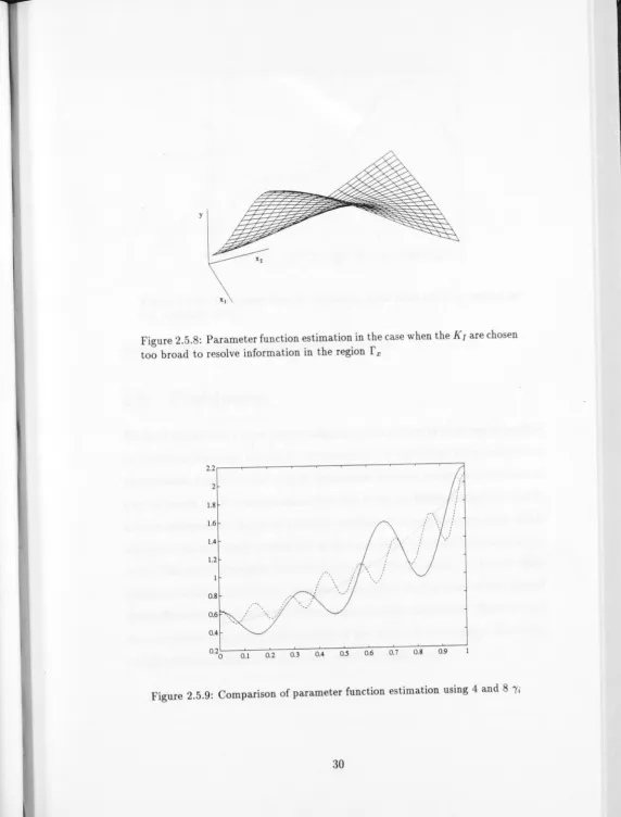
If finer structure is required, it is suggested that extra Ii can be introduced while reducing the spread of KI . A sensible initial value for the associated qi
would be the previous predicted value of 0bi)' This can be seen in Figure 2.5.9,
where an estimate of
x
2-
(x
-
2tl is made using 4 and 8 Ii. The inverse varianceof the interpolating Gaussian was chosen to be 3 times the square of the number
of Ii. This increase in number of interpolating functions corresponds to increasing the size of the class of reconstructible functions and thus decreasing the necessary
error.
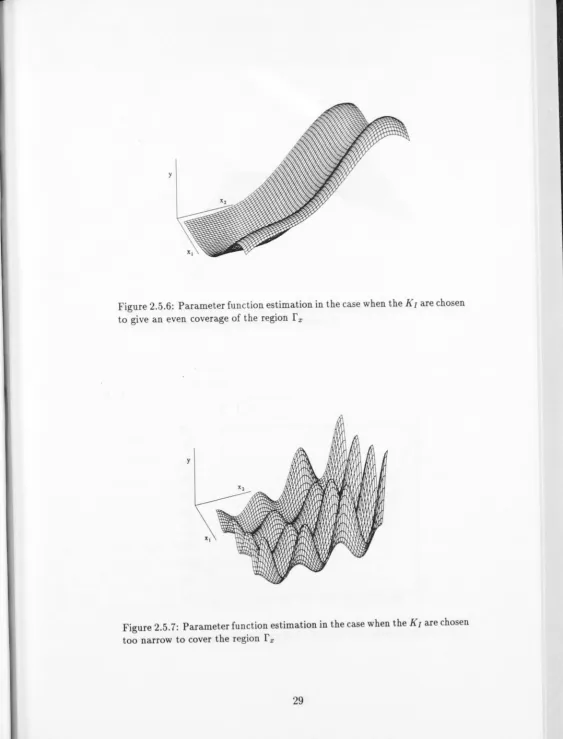
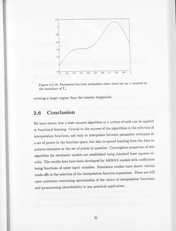
The positioning of the interpolating functions influences the precision of the
function estimation in the case where the function is not reconstructible. If the
Ii are uniformly distributed in the domain and the Kl are fixed bisigmoids then
edge effects are observed, as shown in Figure 2.5.10, which estimates the same surface as Figure 2.5.6, but with II now uniformly distributed over the interior
of the region. This can be prevented by placing Ii on the edge of the domain
y
Figure 2.5.6: Parameter function estimation in the case when the Klare chosen
to give an even coverage of the region
r
xy
y
[image:44.621.36.608.13.765.2]X,
Figure 2.5.8: Parameter function estimation in the case when the Klare chosen too broad to resolve information in the region
r
x2.2 .--_-r-_--,--_--r_---r_~--,._-,..._-__._-__._-__,
2
\.8
\.6
\,4
\,2
0.8
" .. ~
..
0.6 ,,/' " .. ,,: "
0.4
0.20 0.1 0.2 0.3 0.4 0.5 0.6 0.7 0.8 0.9
2
1.8
1.6
1.4
1.2
0.8L-....~-...---<---'--~-~-~-~-~-~---.J
[image:45.621.40.606.18.760.2]o 0.1 0.2 0.3 0.4 0.5 0.6 0.7 0.8 0.9
Figure 2.5.10: Parameter function estimation when there are no /i located on the boundary of
r
xcovering a larger region than the interior bisigmoids.
2.6
Conclusion
We have shown how a least squares algorithm or a system of such can be applied
in functional learning. Crucial to the success of the algorithms is the selection of
interpolation functions, not only to interpolate between parameter estimates at
a set of points in the function space, but also to spread learning from the data to
achieve estimates at the set of points in question. Convergence properties of this
algorithm for stochastic models are established using standard least squares
re-sults. The results here have been developed for ARMAX models with coefficients
being functions of some input variables. Simulation studies have shown various trade-offs in the selection of the interpolation function expansions. There are still open questions concerning optimization of the choice of interpolation functions,
Chapter 3
Linear Algebra and Differential
Equations
3.1
The Link - History and Motivation
Part of the motivation for this work comes from a recent paper by Brockett [4]
itself motivated because of the resurgence of interest neural networks are causing
in analog computing. Brockett's paper explores how certain algebraic problems
that have traditionally been solved using digital computers (linear programming,
sorting lists, and diagonalizing matrices) could be solved via ordinary differential
equations (ODE's) using analog computers, or perhaps special purpose digital
computers using parallel processing techniques which simulate analog computers.
In [6] it is shown that the method of solution of certain algebraic tasks are,
in fact, finite samplings of a differential equation. This raises the question as to
whether a differential equation that converges more rapidly may lead to a faster
recursive solution. The task of discretizing a differential equation is not explored
in this thesis, but does motivate an interest in ODE's with different convergence
rates.
The specific algebraic tasks of interest in this chapter are those of finding
classes of balanced realizations of finite-dimensional linear systems. The simplest
clas-sic problem of singular value decomposition (SVD). The next task considered is a generalization of B.C. Moore's balanced realization [22]. Finally, we are interested
in a new class of balanced realizations (euclidean norm balancing) formulated by Helmke [10]. Further generalizations of algorithms to perform balanced
realiza-tion and balanced matrix factorization are developed in the following chapters. For the SVD and balanced realization tasks, there are efficient algebraic meth-ods of solution and although the ODE methods appear to have certain attractions associated with exponential behaviour, superiority of the ODE techniques pre-sented here is not claimed, based on the author's current knowledge. However, in the third norm minimization task, there are, as yet, no algebraic methods for constructing the associated balanced realization class, and so clearly the ODE
approach is worth exploring in some detail.
3.2
Gradient Flows
For each of the algebraic tasks, as in [4], we associate an ODE
x
=
J(x) with the property that for any x(O), it evolves to a state x(oo) which characterizes the desired solution. The differential equations considered in this thesis are all derived from gradient flows. Gradient flows associate a "case', or Lyapunov Junction, with each point and then define a differential equation that aims to reduce the "cost".A differential equation defined in this manner is more simple to study in terms
of existence and convergence properties.
The properties to be described depend on gradient flows and Lyapunov
func-tions. Any system that can be represented as