This is a repository copy of A new formulation for latent class models. White Rose Research Online URL for this paper:
http://eprints.whiterose.ac.uk/78914/
Monograph:
Brown, S., Greene, W. and Harris, M.N. (2014) A new formulation for latent class models. Research Report. 2014006 . Department of Economics, University of Sheffield ISSN 1749-8368
Reuse
Unless indicated otherwise, fulltext items are protected by copyright with all rights reserved. The copyright exception in section 29 of the Copyright, Designs and Patents Act 1988 allows the making of a single copy solely for the purpose of non-commercial research or private study within the limits of fair dealing. The publisher or other rights-holder may allow further reproduction and re-use of this version - refer to the White Rose Research Online record for this item. Where records identify the publisher as the copyright holder, users can verify any specific terms of use on the publisher’s website.
Takedown
If you consider content in White Rose Research Online to be in breach of UK law, please notify us by
A New Formulation for Latent Class Models
Sarah Brown
William Greene
Mark N. Harris
ISSN 1749-8368
A New Formulation for Latent Class Models
∗
Sarah Brown
aWilliam Greene
bMark N. Harris
ca
Economics Department, University of She¢eld;
b
Economics Department, Stern Business School,
New York University;
c
School of Economics and Finance, Curtin University
April 2014
Abstract
Latent class, or …nite mixture, modelling has proved a very popular, and relatively easy, way of introducing much-needed heterogeneity into empirical models right across the social sciences. The technique involves (probabilisti-cally) splitting the population into a …nite number of (relatively homogeneous) classes, or types. Within each of these, typically, the same statistical model applies, although these are characterised by di¤ering parameters of that distri-bution. In this way, the same explanatory variables can have di¤ering e¤ects
across the classes, for example. A priori, nothing is known about the
behav-iours within each class; but ex post, researchers invariably label the classes
according to expected values, however de…ned, within each class. Here we propose a simple, yet e¤ective, way of parameterising both the class prob-abilities and the statistical representation of behaviours within each class, that simultaneously preserves the ranking of such according to class-speci…c expected values and which yields a parsimonious representation of the class probabilities.
JEL Classi…cation: C3, D1, I1
Keywords: Latent class models, …nite mixture models, ordered probability models, expected values, body mass index.
∗We are grateful to the Data Archive, University of Essex, for supplying the British Household
1
Introduction and Background
Latent class, or …nite mixture, modelling has been applied in a wide variety of areas
of economics ranging from consumer behaviour (see, for example, Reboussin, Ip,
and Wolfson 2008, Chung, Anthony, and Schafer 2011), to health economics (see,
for example, Deb and Trivedi 2002, Bago D’Uva 2005b, Bago D’Uva 2005a) to
trans-port mode choice (see, for example, Shen 2009) as a relatively straightforward way
of introducing much-needed unobserved heterogeneity into empirical models right
across the social sciences. For example, they typically represent a much more
par-simonious representation of such heterogeneity than a standard random parameters approach, and moreover lend themselves to a much richer characterisation of the
data under consideration by being able to group relatively homogeneous individuals
into probabilistically de…ned, but unobserved, classes (or types, or clusters).
The technique involves (probabilistically) splitting the population into a …nite
num-ber of (relatively homogeneous) classes, or types. Within each of these, typically,
the same statistical model applies, although these are characterised by di¤ering
pa-rameters of that particular distribution. In this way, the same explanatory variables
can have di¤ering e¤ects across the classes.
Particularly with respect to examples of such empirical models in economics, several
(related) estimation strategies are invariably employed. Firstly, although a priori
nothing is known about the behaviours within each class, ex post researchers
invari-ably label the classes according to expected values (EVs), however de…ned, within
each class. Secondly, class probabilities do not respect the eventual labeling and
ordering of the classes by EV. Instead, they are estimated using multinomial logit
probabilities, which can be become very heavily parameterised as the number of
potential classes considered rises. And …nally, the optimal number of unobserved
classes is determined by a combination of model selection (or information) criteria
(IC) and model (non-)convergence.1 As IC metrics contain a penalty term for the
1As an excellent example of an application of latent class modelling, and also as an example of
number of parameters estimated, they will clearly be a¤ected by a non-parsimonious
representation of the class assignment probabilities.
Here we propose a simple, yet e¤ective, way of parameterising both the class
prob-abilities and the statistical representation of behaviours within each class, that
si-multaneously preserves their ranking according to class-speci…c expected values and
which yields a parsimonious representation of the class probabilities. Explicitly
we enforce ordering in the EVs across classes and suggest an ordered probabilistic
speci…cation for the class assignment probabilities, that is both consistent with the
ordering in the EVs across classes and o¤ers a much more parsimonious
represen-tation of the class assignment probabilities.
The model proposed here bears some super…cial resemblance to that in Yang, O’Brien, and Dunson (2011), whose speci…cation posits a latent class structure that governs
the allocation of individuals to class speci…c subpopulations Fj. The (stochastic)
ordering aspect of the model applies toFj, not to the classes. One speci…cation
(dis-carded as insu¢ciently general) has Fj a normal population with ordering imposed
on the means. The class allocation mechanism, their equation (4), is a multinomial
(unordered) logit model extended to accommodate unobserved heterogeneity. In our
speci…cation, the ordering applies to the class allocation equation. The underlying
implication being that class allocation itself is governed by positioning on the latent
index. The class speci…c population is characterised by, in this case, a generic linear regression model.
Our approach is generally applicable to the analysis of any output variable which
em-bodies a notion of ordering (either cardinal or ordinal). We illustrate our proposed
technique with an example drawn from the existing health economics literature,
which relates to modelling obesity levels as re‡ected by body mass index (BM I).
The results show a clear preference for the suggested approach over standard ones.
We also undertook a small Monte Carlo experiment which showed the fragileness of
existing techniques and the robustness of the newly suggested approach. In short, regardless of the true data generating process considered for the class-assignment
ap-proaches.
2
Econometric Framework
In a standard latent class model (LCM) the random variable of interest, is
as-sumed to be drawn from a population ofQunknown and unobserved subpopulations,
with corresponding mixing proportions πq. Thus the overall density for individual
i (i= 1, . . . , N), f(yi|xi,θ), is an additive mixture density of Q distinct densities
weighted by their appropriate mixing probabilities πq. The πq are de…ned such that
PQ
q=1πq = 1 and πq ≥ 0 ∀q, q = 1, . . . , Q. The outcome variable of interest is yi,
a¤ected by the (kx×1)vector of covariates in the model, xi, and where θ denotes
all of the parameters of the model.
We will assume the existence of Q latentclasses, or types. These are heterogeneous
across classes as to how they react to observed covariates, but homogeneous within
each class. The corresponding mixture density is
f(yi|xi, π1, . . . , πQ;θ1, . . . , θQ) = Q
X
q=1
πq×f(yi|xi, θq). (1)
The usual approach to address estimation ofπqis to use a multinomial logit(M N L)
form of the probabilities of these, given by
πq =
exp(γq)
PQ
a=1exp(γa)
, (2)
whereγq(= 1, ..., Q)is a set of constants that are used to calculate class probabilities,
and exp() is the exponential function, and where one of the γq is normalised to
zero. However, the choice of functional form for this class assignment function
is clearly inconsequential when class probabilities are treated as constants across
individuals. However, this is not so when one considers an extension to this model
that is increasingly used when the researcher has some prior reasoning as to the
determinants of class membership; this involves an explicit parameterisation of the
lines of the M N Lmodel this would become:
πq =
exp(z′
iγq)
PQ
k=1exp(zi′γk)
(3)
where zi is a(kz×1) vector of explanatory variables that help allocate individuals
to each of the unobserved classes. TheM N Lspeci…cation is evident in most (if not
all) studies where class assignments are expressed as prior functions of covariates
(“generalised”). Indeed, all modern econometric software estimates generalised
la-tent class models in this manner.2 Estimation can now be undertaken, using either
theEM algorithm, or standard maximum likelihood techniques, based on equations
(1) and (3).
After estimating potentially numerous variants of the LCM with regard to the
possible number of (unknown) classes, the researcher will then clearly be faced with
the choice of the most appropriate Q, Q∗. There are non-trivial issues here with
regard to statistical testing across di¤erent values of Q∗ = 1, . . . versus any other
potential value: for example, in testing the null of Q∗ = 1 versus the alternative
of Q∗ = 2, then under the null γ (and therefore neither π
q) is (are) identi…ed.
Presumably for this reason, and moreover because the choice is essentially a model
selection one, researchers invariably rely on the so-called information criteria (IC)
metrics. These are a standard method of choosing across (potentially) non-nested
models (although this is not a prerequisite). Speci…cally, with regard to choosing
the optimal number of classes, the technique involves choosing Q∗ such that
Q∗ = arg min
Q IC(Q), (4)
where:
IC(Q) =−2ˆℓQ+λNpQ; (5)
λN is a deterministic function of N; and pQ is the total number of parameters
estimated in the Q class LCM. Some common choices ofλN include the following:
λN = lnN BIC/SC (Schwarz 1978)
λN = 2 AIC (Akaike 1987)
λN = 1 + lnN CAIC (Bozdogan 1987)
λN = 2 ln lnN HQIC (Hannan and Quinn 1979).
(6)
2To the best of the authors’ knowledge. We use the term “generalised” here to denote the case
These criteria are derived from di¤ering principles and as a result have di¤ering
properties; for example AIC has been shown to favour “large” models (see, for
example, Hurvich and Tsai (1989)). There is no general agreement on the optimal
criterion in the LCM setting, although there seems to be an empirical preference
for AIC (despite - because of? - its preference for large models).
Post model estimation two estimates of the probability of class membership are
available; prior probabilities are obtained by simply evaluating equations (2) or (3).
However, more common, are the posterior, or based on the data, probabilities such
that
Pr (qi|yi) =
πq zi, γq ×f(yi|xi, θq)
PQ
k=1πk(zi, γk)×f(yi|xi, θk)
. (7)
The posterior probabilities answer the question: given that we observe yi what it is
the probability that the individual belongs to class q?
Our point of departure concerns the speci…cation of fq(yi|xi, θq). Clearly the data
at hand will dictate the functional form for the speci…cation of this density: ifyi is a
stochastic count, a Poisson or a Negative Binomial would be appropriate; an ordered
discrete variable - an Ordered Probit/Logit; a censored continuous variable - a Tobit formulation; a continuous variable - a linear regression function; and so on. However,
a de…ning feature of many empirical examples of LCMs is an ex post labelling of
the Q classes based upon estimated EVs within each of the q = 1, . . . , Q classes.
Where ordinality exists, but there are no obvious EV s as such (for example in an
Ordered Probit model) researchers might label classes according to the distribution
of predicted probabilities at the “low” to the “higher” ends of the choice set.
It is useful here, to consider the determination of observedyiwithineachq= 1, . . . , Q
class. We consider a latent index function of the form
y∗
i;q=x′iβq+εi;q (8)
where βq are the response parameters and εi;q a disturbance term. For example, if
there were no subpopulations we would have the set-up of
y∗
The y∗
q of equation (8) will be related to observations within group yi;q via a
map-ping dictated by f(yi|xi, θq). That is, in a linear regression model, yi;q = yi;q∗ . In a
Tobit setting, yi;q = max 0, yi;q∗ . And so on. Regardless of the model, EVs (or
probabilities for models such as the Ordered Probit) on the assumption of
underly-ing ordinality or cardinality of observed yi, are monotonically related to the index
x′
iβq: ensuring that x′iβq=1 ≤x′iβq=2 ≤ ≤x′iβQ will therefore be a necessary and
su¢cient condition to ensure that EVi;q=1 ≤ EVi;q=2 ≤ ≤ EVi;Q. For example,
take the case of health-care utilisation addressed in Bago d’Uva and Jones (2009).
The authors are interested, for example, in whether “low users” are more (or less)
income elastic than “high users”. That is, they wish to …rstly identify high and
low use classes, and then to ascertain whether the drivers across these classes di¤er
in magnitudes (and/or directions of e¤ects). So, clearly the ranking of the classes (by expected values) is paramount in Bago d’Uva and Jones (2009), as well as in
(nearly) all of the related literatures, as is the identi…cation of these classes. Thus
although in Bago d’Uva and Jones (2009) these classes are labelled ex post, below
we suggest an easy way in which this can be enforced in estimation.
By de…ning genericallyEV∗
i;qas the indexx′iβq(positively, and monotonically related
to the trueEV, EVi;q), then this implicit ordering can be enforced via an estimation
strategy as
EV∗
i;q=1 = EVi;q=1 (10)
EV∗
i;q=2 = EVi;q∗=1+ exp x′iβq=2
EV∗
i;q=3 = EVi;q∗=2+ exp x′iβq=3
.. . = ...
where the speci…cation of EVi;q=1 is likely to be model-speci…c. For example, in
a linear regression EVi;q=1 = x′iβq; whilst in a count Poisson regression EVi;q=1 =
exp x′
iβq ; and so on. This is convenient in that ordering is ensured, it is applicable
to a wide range of models, and has the added bene…t that βq,q >2, can be directly
interpreted as di¤erential e¤ects with respect to EV∗
i;q−1. Moreover, any variables
that have no di¤erential e¤ects across neighbouring EV∗
qs are likely to manifest
Thus far we have shown how to enforce ordering with respect to expected values
(broadly de…ned) in a latent class set-up. We now turn to the identi…cation of the
class probabilities. In the literature, there appear to be two major stands of how to address these. Firstly some authors do not wish to explain these class probabilities
with respect to covariates, but then generally ex post attempt to explain the (now
individual-varying) posterior probabilities of class membership by regressing them
on a range of observed characteristics. However, if signi…cant correlations are found
in this second step, in some instances this could well cast doubt on the validity of
the results from the …rst step. That is, model estimation and ex post estimates
of quantities of interest, including estimates of the posterior probabilities, as this
(these) would appear to be based on a mis-speci…ed model. In general we would
expect that the e¤ect of omitted factors (variables) in a model is transmitted to the results estimated for the included factors (variables), in ways that are typically hard
to predict, but regardless are likely to result in biased and mis-speci…ed models.
If one has a notion that the classes are driven by observables, then clearly these
should be allowed for in the modelling process. Indeed, as noted, it is possible
that by ignoring these variables in estimation biased and mis-speci…ed models will
result. Researchers who take this approach (that is, entertaingeneralised latent class
models) generally take the view that the classes, or types, are time-invariant (a kind
of a “…xed e¤ect”) and therefore best explained by any time-invariant variables available to the researcher.
Therefore, on the assumption that the researcher is parameterising the classes
(pre-sumably with respect to time-invariant variables), it is possible to reconsider the
speci…cation of the functional form for these probabilities. This are usually
speci-…ed in the M N L form as per equation (3) above. This may be less than optimal
for several important reasons. Firstly, it appears to represent a description of the
probabilities that does not take advantage of the subsequent ordering applied to the
estimated classes. Secondly, theM N Lform embodies the undesirableIndependence
from Irrelevant Alternatives property.3 Here this would imply that the odds ratio
of the probability of any one class membership relative to any other, is independent
of any additions to, or deletions from, the choice set. The probability of say, an
individual being in class 1 (however labelled) relative to class 2, is independent of
the possible existence of classes 3, 4 and 5. Clearly, asa priori the number of classes
is unknown, this appears to be a somewhat untenable assumption. Indeed, in any
other choice modelling situation, a M N L model approach would be unlikely to be
considered.
The …nal reason why we believe that M N L class probabilities might not be ideal,
relates to the number of estimated parameters such an approach entails: each
addi-tional class mandates an addiaddi-tionalkz parameters in the class assignment equations.
This can have two adverse related consequences. Firstly, this can result in a very
highly parameterised model for even small values ofQwhich will often cause
numer-ical convergence problems. The true model with Q∗ classes, whereQ∗ is a “large”
number, might not even enter the researcher’s potential choice set due to numerical
convergence issues. The second reason why a highly parameterised model, such as
theM N L, might not be an ideal representation of the class assignment equation(s),
relates to the IC metrics invariably used to determine the appropriate number of
classes. As shown in equation(s) (3) above, all such metrics are “adversely” a¤ected
by the penalty term (λNpQ), which regardless of the metric, is an increasing
func-tion ofpQ.That is, theIC’s all depend on pQ, and since the model size is not being
determined by the likelihood statistic, but rather by the IC, there is a premium on
parsimony: this puts the M N L form at a disadvantage compared to a more
com-pact model. These two issues (of non-convergence and a largerICpenalty function)
could jointly, or independently, result in a selectedQ∗ that is “too small”, and hence
potentially bias any subsequent …ndings. Indeed, in the bulk of such empirical
exam-ples ofLCM swe witness a preponderance of values ofQ∗ ≤3.Consider, once more,
the case of health-care utilisation considered by Bago d’Uva and Jones (2009). This
research attempted to uncover the “true” number of underlying classes of individuals
with respect to health-care utilisation, and moreover to ascertain any behavioural di¤erences across the so identi…ed classes (with a focus on income). Thus in using
classes would have been identi…ed, and that on this basis class-speci…c results might
have been contaminated by a merging of heterogeneous classes.4
For all of the above reasons, we propose replacing the M N L probabilities with
Ordered Probit (OP) ones (Greene and Hensher 2010). With the parameterisation
suggested above of equation(s) (10) our class equation output variables y∗
i;q will
necessarily be ordered by EV∗
q, such that such an OP formulation for the class
probabilities will be internally, and explicitly, consistent with this ordering.
By de…ning an unobserved latent variable, q∗
i as a driver of the unobserved classes,
itself a function of observed characteristics zi with unknown weights γ and a
(stan-dard normally distributed) error termui,thenOP probabilities of class membership
can be derived along the following lines. Let q∗
i be of the form
q∗
i =zi′γ+ui, (11)
where zi has no constant term (for normalization). This latent variable translates
to the (here, unobserved) ordered, discrete, class outcomes qi (qi = 1,2, ..., Q) via
the mapping
qi =q 1 q−1 < qi∗ ≤ q ,
where −∞ = 0 < 1 < . . . < Q−1 < Q = ∞ are the boundary parameters with
= 1, . . . , Q−1
′
to be estimated in addition to γ. Under the assumption of
normality, the OP probabilities are given by
f(qi|zi;θOP) = Φ qi−z
′
iγ −Φ qi−1−z
′
iγ ,
where θ = (γ, ).
Moreover whereas theM N Lapproach is based upon an underlying system of Q−1
latent utility equations (Greene 2012), and henceQ−1parameter vectors, theOP is
based upon a single utility index with accordingly a single unique set of parameters
per covariate. Increasing the number of classes in a OP set-up simply requires
estimation of one additional boundary parameter, and not kz as in the M N Lone.
4The authors state that they only considered at most a 2-class model; although not stated this
3
Application: Body Mass Index
Given the serious health related issues associated with obesity, it is not surprising
that modelling body mass index (BM I)and obesity rates are attracting increasing
interest from both academics and policy-makers. Furthermore, as reported by the
World Health Organisation (W HO) in 2011, since 1980, adult obesity rates have
doubled worldwide. It is important to select an appropriate modelling approach
in the context of such an important and highly relevant policy application. The
determination of BM I levels have previously been addressed in the literature using
a latent class framework (Greene, Harris, Hollingsworth, and Maitra 2014). The justi…cation of such an approach here was based on medical evidence that an
obe-sity predisposing genotype is present in 10% of individuals (Herbert, Gerry, and
McQueen 2006): that is, it is (medically) very likely that individuals are genetically
predisposed to being in di¤erent BM I classes.5
We analyse data drawn from the British Household Panel Survey (BHP S). The
BHP S is a longitudinal survey of private households in Great Britain, 1991 to 2008,
and was designed as an annual survey of each adult member of a nationally
represen-tative sample. The …rst wave in 1991 achieved a sample of some 5,500 households,
covering approximately 10,300 adults from 250 areas of Great Britain. The same individuals are re-interviewed in successive waves and, if they split o¤ from their
original households are also re-interviewed along with all adult members of their new
households. The BHP S is a rich source of information on labour market status,
socio-demographic and health variables. In waves 14 (2004) and 16 (2006),
informa-tion was collected on weight and height, which we use to calculate individuals’BM I.
Accordingly our data set comprises of 22,430 observations covering individuals aged
16 and over. The average BM I in the sample is 27.06, with a standard deviation of
5.45 (Table 1), which lies in the lower end of the overweightBM I category suggested
by the W HO.
5We note here that health professionals may not deemBM I an ideal measure of weight-related
As justi…ed above, we treat class membership as time-invariant and search for
prox-ies for di¤erent genetic types to explain membership of these classes. Following
the related literature, we include all available time invariant characteristics, such
as birth cohort, gender and ethnicity.6 In the outcome equation, we again follow
the received literature (see, for example, Cutler, Glaeser, and Shapiro 2003, Chou,
Grossman, and Sa¤er 2004, Brown and Roberts 2013, Greene, Harris, Hollingsworth,
and Maitra 2014) and control for age, number of children, marital status, household
income, employment status, highest level of educational attainment, number of
ciga-rettes smoked per day and a binary indicator for being active (speci…cally whether
the individual walks, swims or plays sport at least once a week). Finally, we also
in-clude a set of eleven controls capturing a wide range of health problems, namely
problems with: arms, legs, hands, etc.; sight; hearing; skin conditions/allergy;
chest/breathing; heart/blood pressure; stomach or digestion; diabetes; anxiety,
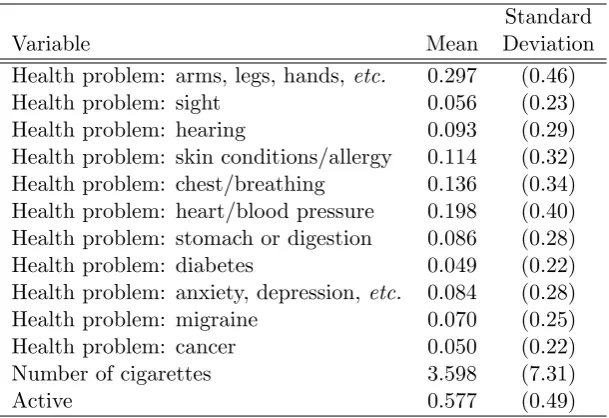
de-pression,etc.; migraine; and cancer.7 Descriptive statistics for the variables included
in the empirical analysis are presented in Tables 1 and 2. In brief, the sample is
evenly split by gender; just over half of the sample are married; and nearly60%are in
full-time employment. The majority of the sample is white, and having a vocational
quali…cation is the most common highest educational attainment category.
Insert tables 1 and 2 about here
We …rstly compare a range of di¤erent models using standardIC metrics in order to
ascertain the preferred approach. We then present detailed estimation results based
on our preferred speci…cation. In order to evaluate the validity of the modelling
approach suggested in Section 2 above, we compare the results from estimating
numerous di¤erent models: we start with a one class linear regression model and then
successively increase the number of latent classes within both a standard framework
(unrestricted) and our new proposed framework (restricted8). We stopped searching
6Unfortunately there are no other, possibly more relevant, time-invariant variables available in
the data.
7We consider the possible existence of reverse causation below.
8Note that here, and subsequently, we use the termrestricted, not so much in the parameteric
for more potential classes when convergence problems were encountered within each
framework. Convergence problems were encountered at Q = 6 for the restricted
approach and 3 for the unrestricted approach. Therefore in total, we consider 6
potential models with regard to the standard IC metrics, which are presented in
Table 3.
TheICmetrics all support the three, four and …ve latent class restricted models (i.e.,
using the newly suggested approach) over the two latent class unrestricted model
(the current standard approach). This supports the modelling approach detailed
in Section 2 above. The AIC and HQIC support the …ve latent class restricted
model over the four latent class restricted model, whilst the BIC and CAIC do
the opposite. In addition to the IC metrics we also look at simple correlations
of the actual versus (prior probability weighted) predicted values for each model.
This is labelled Correlation in Table 3. From these, we can see that the degree
of correlation between the actual and the predicted values increases as we move
from the one class to the …ve latent class restricted model, which further endorses
the modelling approach detailed in Section 2. Based on a combination of the IC
metrics and the correlation of actual versus predicted values, we take the restricted
5-class model as our preferred speci…cation.
Insert table 3 about here
Table 4 presents the increasing pattern in the EVs from classes 1 to 5 for the
restricted …ve latent class model and from classes 1 to 2 for the unrestricted two
latent class model.9 TheEVs for classes 4 and 5 lie in the obese range de…ned by the
World Health Organisation (WHO) as a BM I of 30 and above. Indeed, worryingly,
for class 4, the average posterior probability is “large” (at 0.22), suggesting that a
large proportion of the population lie in this class. On the other hand, only 6% of
the population is estimated to be in the top BM I range. The dispersion within
these classes is relatively large, at 3.8 (σ4 = exp (1.333)) and 5.9 (σ5 = exp (1.767))
9Note that these are evaluated at sample means of covariates, and for the overall value, weighted
respectively, for classes 4 and 5 (compared to the dispersion in the earlier classes).
Only 6% of individuals are estimated to be in the lowest BM I class, with a tight
distribution(σ1 = 1.9) ;with anEV of just over 20, this would class these (according
to the WHO) in the low end of normal weight. Nearly 30% of individuals are
estimated to be in the upper end of normal (WHO classi…ed as18.5−24.9)with an
EV of 23. However, the largest class(40%) would be WHO classi…ed as overweight
(EV = 26), with a variability larger than the lower classes, but smaller than the
higher ones (σ3 = 2.5).
These …ndings are quite distinct from the estimates from the traditional approach.
With EV s at 25 and 32, these distributions are quite dispersed (with σ1 = 3.3
and σ2 = 5.9), which could be hiding the additional classes uncovered by the new
approach. We re-visit this below, but one possible explanation is theM N Lapproach
is su¤ering from convergence problems as a result of “over-…tting” such that it cannot
entertain the “true” number of classes.
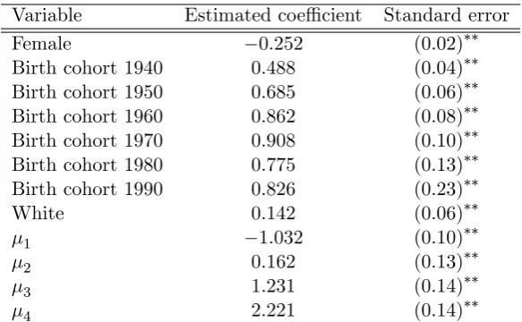
The class membership equation is reasonably well-speci…ed (see Table 5), with the
birth cohort controls generally driving the statistical signi…cance.
Insert tables 4 and 5 about here
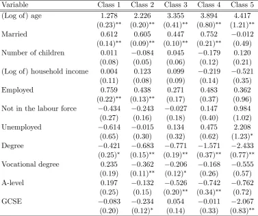
In Tables 6 and 7, we present the partial e¤ects associated with our preferred …ve class restricted model (for demographic, and health-related variables, respectively).
As would be expected, the partial e¤ects di¤er quite dramatically across the …ve
classes in terms of both size and statistical signi…cance. In the case of age, the partial
e¤ects are positive and statistically signi…cant in all …ve classes and increasing in
magnitude from class 1 to class 5. The e¤ect of being married follows a less distinct
pattern, with the partial e¤ects being positive and statistically signi…cant in classes 1
to 4. A reduction in the magnitude of the e¤ect is apparent from classes 1 to 3, then
increasing in the case of class 4. Being employed has a signi…cant positive e¤ect in classes 1 and 2 only. Having a degree as the highest level of educational attainment
with a statistically signi…cant negative e¤ect found for classes 2 to 5, which becomes
more pronounced from classes 2 to 5. The number of cigarettes smoked is inversely
associated with BM I in classes 1 to 5, with the largest inverse e¤ect found in class
5.
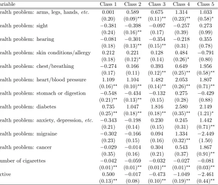
Being active is positively associated with BM I in class 1 and inversely associated
with BM I in classes 3 to 5. With respect to this variable as well as the health
con-dition ones, we note the potential for reverse causation and that our …ndings relate
to correlations rather than causal relationships. As expected due to the di¤erences
associated with the various health conditions, there is a wide degree of variability
in terms of the partial e¤ects with respect to sign, magnitude and statistical
sig-ni…cance. For example, having a heart problem is positively associated with BM I
across all …ve classes, with the largest e¤ect observed in class 4, whereas the e¤ects
of mental health problems are generally statistically insigni…cant at the 1% level
across the 5 classes.
Insert tables 6 and 7 about here
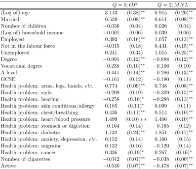
These results illustrate how such an approach(LCM), can highlight interesting
dif-ferential partial e¤ects across classes. However, the latent class approach may be
simply used by some, as a tool to allow for more unobserved heterogeneity into the modelling exercise. Here one would assume that the researcher would be interested
only in overall partial e¤ects, and not those split by class. So, if the overall
par-tials from both the 5-class restricted model and the 2-class unrestricted one were
very similar, it could be argued that our suggested approach has very little bene…t
and/or e¤ect in practice. Table 8 compares the overall (prior probability weighted)
partial e¤ects across the restricted 5-class model and the unrestricted 2-class model.
Although the general pattern of results is broadly consistent across the two models,
there are some substantive di¤erences in terms of size and statistical signi…cance for
a number of explanatory variables (suggesting that using the unrestricted 2-class model may be yielding biased results). For example, age has a much larger e¤ect in
Kernel Densities
<- Xi -> .035
.070 .106 .141 .176
.000
15 20 25 30 35 40 45 50 55 10
BMI OLS
Den
si
[image:18.595.149.447.106.327.2]ty
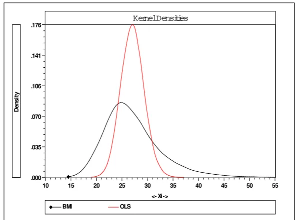
Figure 1: Kernel Densities of Observed BMI and OLS Predictions
statistically signi…cant in the 2-class unrestricted model and statistically
insigni…-cant in the 5-class restricted model. The e¤ects of education, number of cigarettes
smoked and being active are more consistent across the two models although there
are some di¤erences in the magnitudes of the various e¤ects. This is also the case
for the health problems, where they are statistically signi…cant at the 1% level.
Such di¤erences highlight the importance of selecting an appropriate modelling ap-proach especially in the context of policy-relevant applications such as determining
the in‡uences on BM I.
Insert table 8 about here
To further explore behaviours within the estimated classes, and also to ascertain the
overall appropriateness of our approach, we take a closer look at some estimated
densities. Firstly, in Figure 1, we present kernel densities of both the raw BM I
data, and that implied if simple regression techniques had been applied to model it.
Kernel Densities
<- Xi -> .035
.071 .106 .142 .177
.000
20 30 40 50 60 70
10
LC5_1 LC5_2 LC5_3 LC5_4 LC5_5
Den
si
[image:19.595.150.446.106.329.2]ty
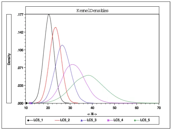
Figure 2: Kernel Density Estimates by Class
In Figure 2 we plot the implied estimated densities by class. The (enforced) ordering in these densities is evident, as their measures of central tendency (and dispersion)
clearly increase over classes 1 to 5. Taken in consideration with their posterior
probabilities, we can see that individuals have a very low chance of being in either
the lowest or the highest BM I range classes. However, individuals in these are
clearly likely to have very low and high, respectively,BM I levels with relatively low
probabilities of having very highBM I values (for class 1) and very low levels (class
5). Interestingly, although freely estimated, the spread of these distributions clearly
also increases with class. An implication of this is that although the highest BM I
range class has a very high EV, it appears that behavioural choices, for example,
can indeed help these individuals into more healthyBM I ranges. On the contrary,
individuals in either of the lowest two classes, appear to be very likely closely bound
to their class-speci…c EV s of low to mid20s.
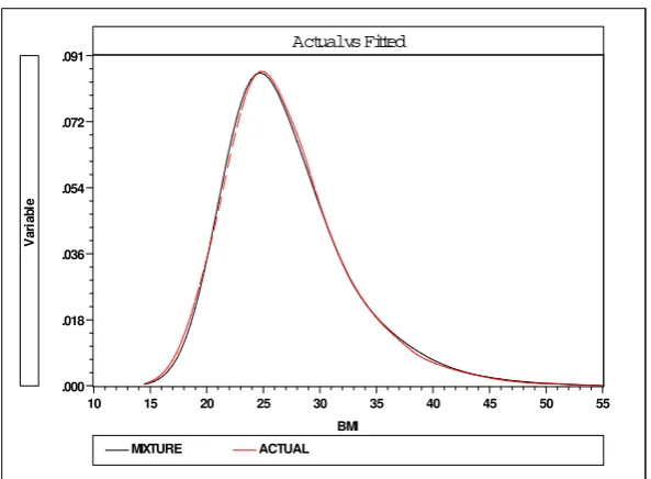
Finally, in Figure 3 we present (prior) probability weighted aggregate predicted
Actual vs Fitted
BMI .018
.036 .054 .072 .091
.000
15 20 25 30 35 40 45 50 55 10
MIXTURE ACTUAL
V
a
ria
b
[image:20.595.151.448.105.323.2]le
Figure 3: Kernel Density Estimates of Actual BM I and Overall PredictedBM I
in predicting the empirical density, especially as compared to a simple regression
approach (Figure 1). Again, we would suggest that this is a further validation of
the suggested approach.
3.1
Robustness Checks
An obvious robustness check against which to compare our model results, is to
consider a constants-only variant, where following much of the LCM literature, the
class-assignment prior probabilities are simply modelled as constants. To this end we
re-estimate our model removing all covariates from the class equations. For reasons
of space, we do not report the full set of results from this exercise.10 However,
in Table 9 we present the model selection metrics from this exercise, along with
the ones for our preferred model. Thus we can see that for all IC measures and
for the values for Correlation, our approach consistently out-performs all possible
contenders for the constants-only version (the overall preferred …gures are presented
inbold, and those for the constants-only versions initalics). There is disagreement
across the IC metricsas to the preferred number of classes, with BIC and CAIC
favouring 3-classes, AIC 5-classes, and HQIC 4-classes. Taking these …ndings in
conjunction with the …t of the model, as de…ned by the correlation values, we take
the 3-class constants-only version as the preferred speci…cation here.
The constants-only approach appears to favour a smaller number of classes, and
in terms of the metrics considered, appears to perform worse than our preferred
approach. However, again, if the researcher is predominantly interested in overall
partial e¤ects, then if the two approaches yield very similar results in this respect,
one would presumably favour the less generalised approach. To address this, in
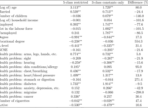
Table 10 we compare (prior probability weighted) overall marginal e¤ects from the 3-class constants-only approach with those previously presented from our preferred
approach. In the …nal column we also present percentage di¤erences in these. It
is clear that the approach undertaken is consequential for these summary partial
e¤ects. For example, we …nd both large absolute and relative, changes in partials
across the approaches, and moreover even changes in signs and signi…cance levels
of e¤ects. For example, the (estimated) e¤ect of age is almost halved; the number
of children turns from insigni…cance to a signi…cantly positive e¤ect (as does “not
in the labour force”); the e¤ect of being employed increases over fourfold; and so
on. However, we also note that large di¤erences are not evident across-the-board:
for example, the e¤ect of the health problem (arms, legs, etc.) remains e¤ectively
unchanged (at 0.774 as compared to 0.732); as does the number of cigarettes smoked
(-0.042 to -0.028); and being active (-0.530 compared to -0.479). We would surmise
that the variables exhibiting the largest di¤erences are probably those most severely
a¤ected by ignoring the omitted covariates in the class equation (that is, presumably
the most highly correlated with the omitted drivers of the class equation); and those
where the change is negligible, would be less a¤ected (and presumably less strongly
related to the omitted class covariates).
The second robustness check we consider, is that in our (BM I)output equation, as
BM I is a¤ected by say, health problems related to breathing. However, clearly the
strong possibility of reverse causation exists here, with the health condition not only
causing the BM I level (in part), but alsoBM I levels (in part) contributing to the
various health conditions. If we had appropriate identifying variables for these health
conditions, that could be considered independent toBM I,we could apply the usual
techniques for allowing for this endogeneity (for example, along the lines of Rivers
and Vuong 1988, Terza, Basu, and Rathouz 2008). As always, such variables are hard
to …nd and justify here, so instead we simply remove those likely o¤ending variables
(all of the health related ones and the activity one) and re-estimate the model.
Reassuringly the results are e¤ectively unchanged. Thus, we still …nd that theM N L
can only entertain up to a 2-class model; whereas theOP approach can go as high as
5. The IC metrics similarly choose both OP 4 - and 5-class over theM N L 2-class
one, and moreover are split between the choice between the two former (whilst the
correlation measure again favours the OP 5-class model). Moreover, class-speci…c
(and overall)EVs, partial e¤ects and posterior probabilities are similarly extremely
close to those models with the potentially endogenous variables included, overall
leading us to the conclusion that the original results were not unduly a¤ected by
endogeneity.
4
Does the
M N L
approach tend to “over-…t”?
The empirical results presented above with regard to the new suggested approach,
and the more traditional (M N L)one, tend to suggest that the latter might be
sub-ject to “over-…tting”, and that this could adversely a¤ect the number of potential
classes one could consider as appropriate. In essentially estimating a separate
equa-tion for each of the classes, it may well be that one, or more, covariates has no, or
little, variation within a particular class, for example. Clearly issues such as this
will adversely a¤ect identi…cation and model estimation.
To ascertain whether this is a likely …nding for our application, we undertook a
obser-vations used in the empirical example (which was held constant for the course of
the experiment), and exactly the same model set-up as above with regard to the
covariates in the model. For estimation purposes this left us with N = 11,203
ob-servations. We explicitly generated the class probabilities via the M N L form, for
a 4-class model, and then estimated the model via the OP and M N L procedures
as described above. Coe¢cients for all parts of the model were simply generated as
random numbers from a (standard) normal distribution, and then held …xed. The
exceptions to this were the constants in the regression equations, which were set at
20,30,40 and 50, to ensure that the EV di¤ered across the four classes, and the
baseline M N Lparameters which, as usual, were normalised to zero.
The results were really quite illuminating. What we found was that whilst the newly
suggested(OP) procedure only encountered convergence problems in15% of cases,
theM N L (the true data generating process) did so in a remarkable 43% of cases.11
Although it would be a stretch to generalise these …ndings to all such M N L class
models, it will clearly be a potential problem in many instances, and one that the
suggested procedure will predominantly circumvent.12
5
Conclusions
Building on the observation that in most empirical examples authors ex post rank
and label their identi…ed classes according to class-speci…c expected values, we
ex-tend the latent class methodology by proposing a procedure that allows for this
ranking in estimation. We also develop a functional form for the class
probabili-ties that is more parsimonious than the familiar multinomial logit model. There
are numerous reasons why the M N L probabilities may not be an ideal choice in
such a situation for the applied researcher (in addition to the fact that it does
not take advantage of the ubiquitous ranking of classes post estimation). These
11Full Monte Carlo results are available from the authors on request. Due to the length of time
to estimate all models, the number of Monte Carlo repetitions was limited to 100.
12Indeed, we did not record in how many instances there was no variation in any variables within
include both the unattractive Independence from Irrelevant Alternatives property
(which appears particularly an issue for latent class modelling), as well as yielding a
very heavily parameterised model. Indeed, it is our conjecture that researchers are quite often restricted in the number of classes they can estimate due to numerical
convergence issues: a case of “over-…tting” (a …nding con…rmed by a small Monte
Carlo experiment). Indeed, in our empirical example, only a two-class variant could
be considered using traditional, M N L, class probabilities, whereas our suggested
approach could estimate up to …ve.
The empirical example attempted to identify an unknown number of inherent classes
with respect to peoples’ weight related health status, orBM I, levels. As noted, the
traditional approach could only estimate a 2-class model, which would have been the preferred model in this case. However, our ordered approach could consider,
and indeed favoured, a much more ‡exible mixing distribution, with up to 5-classes
being supported.
The technique is widely applicable: wherever a latent class model is being applied to
an output variable which embodies any ordinal, or cardinal, ordering. The suggested
approach is only useful if covariates appear in the class probabilities. Otherwise the
proposed model amounts only to a one-to-one reparameterisation. We would also
suggest that, in general, explaining the classes with observed heterogeneity will be
preferable, and will provide more reliable estimates of the posterior probabilities of class membership, and will be less likely to be adversely a¤ected by any omitted
variable bias. Indeed, in the empirical application, using a constants-only approach
References
Akaike, H. (1987): “Information Measures and Model Selection,” International
Statistical Institute, 44, 277–291.
Bago D’Uva, T. (2005a): “Latent Class Models for Utilisation of Health Care,”
Health Economics, 15(4), 329–343.
(2005b): “Latent Class Models for Utilisation of Primary Care: Evidence
from a British Panel,”Health Economics, 14(9), 873–892.
Bago d’Uva, T., and A. Jones (2009): “Health care utilisation in Europe: New
evidence from the ECHP,” Journal of Health Economics, 28, 265–279.
Bozdogan, H.(1987): “Model Selection and Akaike’s Information Criteria (AIC):
The General Theory and its Analytical Extensions,”Psychometrika, 52, 345–370.
Brown, H., and J. Roberts (2013): “Born to be wide? Exploring correlations in
mother and adolescent body mass index,”Economics Letters, pp. 413–415.
Chou, S., M. Grossman,and H. Saffer(2004): “An economic analysis of adult
obesity: results from the Behavioral Risk Factor Surveillance System,” Journal
of Health Economics, 23, 565–587.
Chung, H., J. C. Anthony, and J. L. Schafer (2011): “Latent class pro-…le analysis: an application to stage sequential processes in early onset drinking
behaviours,” Journal of the Royal Statistical Society: Series A, 174, 689–712.
Cutler, D., E. Glaeser, and J. Shapiro(2003): “Why have American become
more obese?,”Journal of Economic Perspectives, 17(3), 93–118.
Deb, P., and P. Trivedi (2002): “The Structure of Demand for Health Care:
Latent Class versus Two-Part Models,”Journal of Health Economics, 21(4), 601–
Fry, T., and M. Harris (1996): “A Monte Carlo Study of Tests for the
Inde-pendence of Irrelevant AlternativesProperty,” Transportation Research - Part B,
30B, 19–30.
Greene, W. (2012): Econometric Analysis 7e. Prentice Hall, New Jersey, USA,
sixth edn.
Greene, W., M. Harris, B. Hollingsworth, and P. Maitra (2014): “A
Latent Class Model for Obesity,” Economics Letters, 123, 1–5.
Greene, W., and D. Hensher (2010): Modeling Ordered Choices. Cambridge University Press.
Hannan, E., and B. Quinn (1979): “The Determination of the Order of an
Au-toregression,”Journal of the Royal Statistical Society, B, 41, 190–195.
Herbert, A., N. Gerry, and N. e. A. McQueen(2006): “A Common Genetic
Variant Is Associated with Adult and Childhood Obesity,”Science, 312, 279–283.
Hurvich, C., and C.-L. Tsai (1989): “Regression and time series model selection
in small samples,”Biometrika, 76, 297–307.
Reboussin, B. A., E. Ip, and M. Wolfson (2008): “Locally dependent latent class models with covariates: an application to under-age drinking in the USA,”
Journal of the Royal Statistical Society: Series A, 171, 877–97.
Rivers, D., and Q. Vuong (1988): “Limted information estimators and
exogene-ity tests for simultaneous probit models,” Journal of Econometrics, 39, 347–366.
Schwarz, G.(1978): “Estimating the Dimensions of a Model,”Annals of Statistics,
6(2), 461–464.
Shen, J. (2009): “Latent class model or mixed logit model? A comparison by
transport mode choice data,” Applied Economics, 41, 2915–24.
Terza, J. V., A. Basu,andP. J. Rathouz(2008): “Two-stage residual inclusion
estimation: Addressing endogeneity in health econometric modeling,”Journal of
Yang, H., S. O’Brien, and D. B. Dunson (2011): “Nonparametric Bayes
Sto-chastically Ordered Latent Class Models,” Journal of the American Statistical
Table 1: Descriptive statistics; demographics
Standard
Variable Mean Deviation
BM I 27.059 (5.45)
Birth cohort 1940 0.158 (0.36)
Birth cohort 1950 0.168 (0.37)
Birth cohort 1960 0.201 (0.40)
Birth cohort 1970 0.160 (0.37)
Birth cohort 1980 0.115 (0.32)
Birth cohort 1990 0.004 (0.06)
Female 0.504 (0.50)
White 0.976 (0.15)
(Log of) age 3.784 (0.42)
Married 0.560 (0.50)
Number of children 0.575 (0.96)
(Log of) household income 10.190 (0.74)
Employed 0.583 (0.49)
Not in the labour force 0.159 (0.37)
Unemployed 0.028 (0.16)
Degree 0.143 (0.35)
Vocational degree 0.286 (0.45)
A-level 0.117 (0.32)
GCSE 0.167 (0.37)
Table 2: Descriptive statistics; health
Standard
Variable Mean Deviation
Health problem: arms, legs, hands,etc. 0.297 (0.46)
Health problem: sight 0.056 (0.23)
Health problem: hearing 0.093 (0.29)
Health problem: skin conditions/allergy 0.114 (0.32)
Health problem: chest/breathing 0.136 (0.34)
Health problem: heart/blood pressure 0.198 (0.40)
Health problem: stomach or digestion 0.086 (0.28)
Health problem: diabetes 0.049 (0.22)
Health problem: anxiety, depression, etc. 0.084 (0.28)
Health problem: migraine 0.070 (0.25)
Health problem: cancer 0.050 (0.22)
Number of cigarettes 3.598 (7.31)
[image:28.595.147.452.515.724.2]Table 3: Model selection metrics
BIC AIC CAIC HQIC Correlation
Linear Regression 138,210 138,014 138,236 138,080 0.2759
2-class (restricted) 134,442 133,982 134,503 134,135 0.2970
3-class (unrestricted) 134,437 133,977 134,498 134,131 0.2975
3-class (restricted) 134,128 133,464 134,216 133,685 0.2001
3-class (unrestricted) − − − − −
4-class (restricted) 134,088 133,221 134,203 133,510 0.3045
4-class (unrestricted) − − − − −
5-class (restricted) 134,160 133,089 134,302 133,446 0.3087
5-class (unrestricted) − − − − −
[image:29.595.86.587.347.472.2]Note: preferred model for each metric in bold.
Table 4: Expected values, averaged posterior probabilities and dispersion parameters
Q= 5;OP Q= 2;M N L Expected P osterior Expected P osterior
V alue probability ln (Dispersion) V alue probability ln (Dispersion)
Class 1 20.37 (0.24)∗∗ 0.06 0.667 (0.06)∗∗ 25.09 (0.05)∗∗ 0.28 1.184 (0.01)∗∗
Class 2 23.24 (0.17)∗∗ 0.27 0.687 (0.05)∗∗ 31.91 (0.20)∗∗ 0.72 1.767 (0.01)∗∗
Class 3 26.46 (0.22)∗∗ 0.39 0.929 (0.04)∗∗ − − −
Class 4 31.27 (0.48)∗∗ 0.22 1.333 (0.04)∗∗ − − −
Class 5 37.61 (0.86)∗∗ 0.06 1.767 (0.05)∗∗ − − −
Overall 26.90 (0.04)∗∗ − − 27.00 (0.04)∗∗ − −
Notes: ∗∗and ∗denote signi…cant at 5, and 10% size, respectively. The preferred model for each
metric inbold.
Table 5: Class membership equation; preferred speci…cation
Variable Estimated coe¢cient Standard error
Female −0.252 (0.02)∗∗
Birth cohort 1940 0.488 (0.04)∗∗
Birth cohort 1950 0.685 (0.06)∗∗
Birth cohort 1960 0.862 (0.08)∗∗
Birth cohort 1970 0.908 (0.10)∗∗
Birth cohort 1980 0.775 (0.13)∗∗
Birth cohort 1990 0.826 (0.23)∗∗
White 0.142 (0.06)∗∗
1 −1.032 (0.10)∗∗
2 0.162 (0.13)∗∗
3 1.231 (0.14)∗∗
4 2.221 (0.14)∗∗
[image:29.595.153.445.540.720.2]Table 6: Class-speci…c partial e¤ects; demographics
Variable Class 1 Class 2 Class 3 Class 4 Class 5
(Log of) age 1.278 2.226 3.355 3.894 4.417
(0.23)∗∗ (0.20)∗∗ (0.41)∗∗ (0.80)∗∗ (1.21)∗∗
Married 0.612 0.605 0.447 0.752 −0.012
(0.14)∗∗ (0.09)∗∗ (0.10)∗∗ (0.21)∗∗ (0.49)
Number of children 0.011 −0.084 0.045 −0.179 0.120
(0.08) (0.05) (0.06) (0.12) (0.21)
(Log of) household income 0.004 0.123 0.099 −0.219 −0.521
(0.11) (0.08) (0.09) (0.14) (0.35)
Employed 0.759 0.438 0.271 0.483 0.362
(0.22)∗∗ (0.13)∗∗ (0.17) (0.37) (0.96)
Not in the labour force −0.434 −0.243 −0.027 0.147 0.984
(0.27) (0.16) (0.18) (0.40) (1.02)
Unemployed −0.614 −0.015 0.134 0.475 2.208
(0.65) (0.30) (0.32) (0.62) (1.23)∗
Degree −0.421 −0.683 −0.771 −1.571 −2.433
(0.25)∗ (0.15)∗∗ (0.19)∗∗ (0.37)∗∗ (0.77)∗∗
Vocational degree 0.235 −0.362 −0.206 −0.168 −0.555
(0.19) (0.11)∗∗ (0.12)∗ (0.26) (0.57)
A-level 0.197 −0.132 −0.526 −0.742 −0.762
(0.25) (0.15) (0.20)∗∗ (0.34)∗∗ (0.72) GCSE −0.083 −0.234 0.054 −0.011 −2.067
Table 7: Class-speci…c partial e¤ects; health
Variable Class 1 Class 2 Class 3 Class 4 Class 5
Health problem: arms, legs, hands,etc. 0.001 0.589 0.675 1.314 1.033
(0.20) (0.09)∗∗ (0.11)∗∗ (0.23)∗∗ (0.58)∗
Health problem: sight −0.381 −0.398 −0.097 −0.257 0.273
(0.24) (0.16)∗∗ (0.17) (0.39) (0.99)
Health problem: hearing −0.081 −0.301 −0.354 −0.218 0.355
(0.18) (0.13)∗∗ (0.15)∗∗ (0.31) (0.78)
Health problem: skin conditions/allergy 0.212 0.221 0.128 0.484 −0.791
(0.18) (0.12)∗ (0.14) (0.26)∗ (0.80)
Health problem: chest/breathing −0.274 0.166 0.393 0.649 1.956
(0.17) (0.11) (0.12)∗∗ (0.25)∗∗ (0.58)∗∗
Health problem: heart/blood pressure 1.109 1.104 1.482 2.053 1.807
(0.16)∗∗ (0.10)∗∗ (0.14)∗∗ (0.26)∗∗ (0.71)∗∗
Health problem: stomach or digestion −0.548 −0.434 −0.132 0.275 −0.429
(0.21)∗∗ (0.13)∗∗ (0.15) (0.28) (0.88)
Health problem: diabetes 0.735 1.047 1.816 2.580 2.149
(0.25)∗∗ (0.18)∗∗ (0.18)∗∗ (0.35)∗∗ (1.21)∗
Health problem: anxiety, depression, etc. −0.343 −0.198 0.230 0.245 1.442
(0.21) (0.14) (0.15) (0.31) (0.71)∗∗
Health problem: migraine −0.302 −0.166 0.094 1.334 −2.449
(0.23) (0.15) (0.16) (0.32)∗∗ (1.50)
Health problem: cancer −0.029 −0.014 0.304 0.543 1.867
(0.35) (0.16) (0.21) (0.37) (0.91)∗∗
Number of cigarettes −0.042 −0.059 −0.032 −0.027 −0.081
(0.01)∗∗ (0.01)∗∗ (0.01)∗∗ (0.01)∗∗ (0.03)∗∗
Active 0.500 −0.017 −0.473 −1.049 −2.461
Table 8: Overall partial e¤ects
Q= 5;OP Q= 2;M N L
(Log of) age 3.113 (0.38)∗∗ 0.915 (0.20)∗∗
Married 0.539 (0.08)∗∗ 0.611 (0.08)∗∗
Number of children −0.036 (0.04) 0.026 (0.04)
(Log of) household income −0.001 (0.06) 0.039 (0.06)
Employed 0.392 (0.16)∗∗ 1.057 (0.13)∗∗
Not in the labour force −0.015 (0.18) 0.431 (0.15)∗∗
Unemployed 0.241 (0.34) 1.015 (0.25)∗∗
Degree −0.991 (0.12)∗∗ −0.888 (0.12)∗∗
Vocational degree −0.238 (0.10)∗∗ −0.106 (0.10)
A-level −0.441 (0.14)∗∗ −0.286 (0.13)∗∗
GCSE −0.161 (0.12) −0.180 (0.11)
Health problem: arms, legs, hands,etc. 0.774 (0.09)∗∗ 0.748 (0.08)∗∗
Health problem: sight −0.209 (0.19) −0.309 (0.15)∗∗
Health problem: hearing −0.258 (0.16)∗ −0.288 (0.13)∗∗
Health problem: skin conditions/allergy 0.185 (0.11)∗ 0.099 (0.11)
Health problem: chest/breathing 0.436 (0.11)∗∗ 0.514 (0.10)∗∗
Health problem: heart/blood pressure 1.499 (0.10)∗ ∗ 1.406 (0.10)∗∗
Health problem: stomach or digestion −0.164 (0.14) −0.165 (0.12)
Health problem: diabetes 1.732 (0.24)∗∗ 1.851 (0.17)∗∗
Health problem: anxiety, depression, etc. 0.152 (0.14) 0.160 (0.15)
Health problem: migraine 0.132 (0.16) −0.120 (0.14)
Health problem: cancer 0.336 (0.19)∗ 0.267 (0.16)∗
Number of cigarettes −0.042 (0.01)∗∗ −0.038 (0.00)∗∗
Active −0.530 (0.07)∗∗ −0.478 (0.07)∗∗
Notes: ∗∗ and∗ denote signi…cant at 5, and 10% size, respectively.
Table 9: Model selection metrics; comparison with constants-only approach
BIC AIC CAIC HQIC Correlation
Linear Regression 138,210 138,014 138,236 138,080 0.2759
5-class (restricted) 134,160 133,089 134,302 133,446 0.3087
2-class (constants) 134,526 134,126 134,579 134,260 0.2748
3- class (constants) 134,319 133,715 134,399 133,916 0.2755
4-class (constants) 134,349 133,542 134,456 133,810 0.2754
5-class (constants) 134,522 133,511 134,656 133,848 0.2753
Note: preferred model for each metric inbold. Preferred model for the constants-only versions in
[image:32.595.100.497.595.693.2]Table 10: Overall partial e¤ects; comparison with constants-only approach
5-class restricted 3-class constants only Di¤erence(%)
(Log of) age 3.113∗∗ 1.729∗∗ 80.0
Married 0.539∗∗ 0.713∗∗ −24.4
Number of children −0.036 0.079∗∗ −146.0
(Log of) household income −0.001 0.054 −101.6
Employed 0.392∗∗ 1.747∗∗ −77.6
Not in the labour force −0.015 1.002∗∗ −101.5
Unemployed 0.241 1.787∗∗ −86.5
Degree −0.991∗∗ −0.844∗∗ 17.3
Vocational degree −0.238∗∗ −0.036 554.3
A-level −0.441∗∗ −0.335∗∗ 31.4
GCSE −0.161 −0.205∗ −21.6
Health problem: arms, legs, hands, etc. 0.774∗∗ 0.732∗∗ 5.8
Health problem: sight −0.209 −0.267∗ −21.9
Health problem: hearing −0.258∗ −0.306∗∗ −15.6
Health problem: skin conditions/allergy 0.185∗ 0.095 95.0
Health problem: chest/breathing 0.436∗∗ 0.532∗∗ −17.9
Health problem: heart/blood pressure 1.499∗∗ 1.317∗∗ 13.8
Health problem: stomach or digestion −0.164 −0.044 271.4
Health problem: diabetes 1.732∗∗ 1.914∗∗ −9.5
Health problem: anxiety, depression, etc. 0.152 0.266∗ −42.9
Health problem: migraine 0.132 −0.066 −298.0
Health problem: cancer 0.336∗ 0.257 30.4
Number of cigarettes −0.042∗∗ −0.028∗∗ 47.4
Active −0.530∗∗ −0.479∗∗ 10.6