Traffic control and route choice; capacity maximization and stability

This is a repository copy of Traffic control and route choice; capacity maximization and

stability.

White Rose Research Online URL for this paper:

http://eprints.whiterose.ac.uk/86664/

Version: Accepted Version

Article:

Smith, MJ, Liu, R and Mounce, R (2015) Traffic control and route choice; capacity

maximization and stability. Transportation Research Part B: Methodological, 81 (3). pp.

863-885. ISSN 0191-2615

https://doi.org/10.1016/j.trb.2015.07.002

© 2015. This manuscript version is made available under the CC-BY-NC-ND 4.0 license

http://creativecommons.org/licenses/by-nc-nd/4.0/

eprints@whiterose.ac.uk https://eprints.whiterose.ac.uk/

Reuse

Unless indicated otherwise, fulltext items are protected by copyright with all rights reserved. The copyright exception in section 29 of the Copyright, Designs and Patents Act 1988 allows the making of a single copy solely for the purpose of non-commercial research or private study within the limits of fair dealing. The publisher or other rights-holder may allow further reproduction and re-use of this version - refer to the White Rose Research Online record for this item. Where records identify the publisher as the copyright holder, users can verify any specific terms of use on the publisher’s website.

Takedown

If you consider content in White Rose Research Online to be in breach of UK law, please notify us by

Please cite this article in press as:

Smith, M.J., Liu, R. and Mounce, R. (2015) Traffic control and route choice; capacity maximization and stability. Full paper accepted for oral presentation at ISTTT21. Transportation Research Part B, accepted on 26th May 2015.

Traffic control and route choice; capacity maximization and

stability

Michael J Smith

, Ronghui Liu

and Richard Mounce

a

Department of Mathematics, University of York, YO10 5DD, York, UK

b

Institute for Transport Studies, University of Leeds, Leeds LS2 9JT, UK

c

School of Geoscience, University of Aberdeen, Aberdeen, AB24 3FX, UK

Abstract

This paper presents idealised natural general and special dynamical models of day-to-day

re-routeing and of day to day green-time response. Both green-time response models are based on the

responsive control policy P0 introduced in Smith (1979a, b, c 1987). Several results are proved. For

example, it is shown that, for any steady feasible demand within a flow model, if the general day to

day re-routeing model is combined with the general day to day green-time response model then under

natural conditions any (flow, green-time) solution trajectory cannot leave the region of supply-feasible

(flow, green-time) pairs and costs are bounded. Throughput is maximised in the following sense.

Given any constant feasible demand; this demand is met as any routeing / green-time trajectory

evolves (following either the general or the special dynamical model). The paper then considers simple “pressure driven” responsive control policies, with explicit signal cycles of fixed positive duration. A possible approach to dynamic traffic control allowing for variable route choices is

outlined. It is finally shown that modified Varaiya (2013) and Le at al (2013) pressure-driven

responsive controls may not maximise network capacity, by considering a very simple one junction

network. It is shown that (with each of these two modified policies) there is a steady demand within

the capacity of the network for which there is no Wardrop equilibrium consistent with the policy. In

contrast, responsive P0 on this simple network does maximise throughput at a quasi-dynamic user

equilibrium consistent with P0; queues and delays remain bounded in natural dynamical evolutions in

this case. It is to be expected that this P0 result may be extended to allow for certain time-varying

demands on a much wider variety of networks; to show that this is indeed the case is a challenge for

the future.

1.Introduction

It is important

(1) to use traffic signal control to make good use of the capacity of a given road network and

(2) to do the best to ensure that the network, with the traffic control operating, is stable.

This paper considers both (1) and (2) within a day to day model with various responsive signal setting

strategies.

First the paper considers, in sections 2-4, two simple dynamical [flow + green-time] models

involving route flows and signal green-times in which the signal adjustments seek to ensure that consequent natural travellers’ re-routeing decisions make the best utilisation of the capacity available on a given road network. In these two models (which we call “the general model” and “the special model”) signal setting changes actively encourage congestion-reducing route-swaps in the future; both

models maximise network capacity under natural conditions. The capacity maximising effect arises

because both models utilise the P0 signal control policy. This policy has been studied previously (see

Smith (1979a, b, c, 1987, 2011), Smith et al (1987), Smith and Ghali (1990), Smith and van Vuren

(1993), Smith and Mounce (2011), Smith (2015) and Liu and Smith (2015). Both the performance and

stability of the re-routeing – control interactions is considered. The dynamical models here, in sections

2-4, do not involve explicit queues.

Then, in sections 5-8, distributed traffic control / routeing models involving explicit queues are

considered. Here the signal control policies include not only P0 but also naturally modified versions of

control policies suggested by Varaiya (2013) and Le et al (2013); here called policy MV and policy

ML. It is shown that neither MV nor ML are certain to maximise network capacity when travellers are

free to choose their own routes, by displaying a network where neither of these control policies is

consistent with equilibrium route choices by drivers: natural corresponding day to day models give

rise to ever-increasing queues (if users continually swap to cheaper routes). It is shown that, on the

other hand, the P0 policy does maximise the capacity of this network at a user-equilibrium routeing

pattern, where all drivers are on cheapest routes: queues are then bounded in natural day to day

models.

The policies suggested by Varaiya (2013) and Le et al (2013) are both motivated by the paper by

Tassiulas and Ephremides (1992); on stability in the control of constrained queueing networks. This

initial work was aimed at ensuring queueing stability (and maximum throughput) in multi-hop radio

networks. In these networks only certain sets of nodes are allowed to transmit simultaneously due to

power and interference limitations. These sets of nodes are rather like signal stages at junctions where

1.1.Outline description and purpose of the day to day control/routeing models introduced here

The central control variables in severely congested networks are green-times; these are the

proportions of time different links and stages are given green. We also (especially in sections 2-4)

utilise red-times rather than green-times: using red-times gives an intuitive way of adding signal

timings into traffic routeing models.

Sections 2-4 obtain capacity-maximization and stability results. In these sections the central formula for the “pressure” on a stage arises from the P0 signal setting policy. It is shown (in sections 2

– 4) that with this policy the routeing – control dynamical loop is both capacity maximising and stable for a general network without queues. Sections 5-8 show that other policies do not necessarily have

this capacity-maximisation property.

Each dynamical [routeing and signal setting] model described in this paper may be regarded as a

model of a system periodically updated by some new choices of route (by say car drivers) and some

new choices of signal timings (by a signal engineer or by an automatic control system). To be specific

in this paper we generally think of both the route choice and signal control dynamics as operating from day to day. (A more general context is possible: this is “epoch to epoch”. In this case both short -term within day route swapping and longer -term week to week or month to month route swapping may

be considered, very approximately along the lines described here.)

Route flow changes (in the general and the special model) are driven by the following principle. On

each day:

for each route with positive flow yesterday, some of that flow may swap today

but only to a route which was less costly yesterday (and joins the same OD pair). (1.1)

This is a natural if rather conservative behavioural assumption and depends on the definition of route

cost. There is here no compulsion to swap route-flow; yesterday’s route flows are permitted to remain

the same today. (Both the route-choice models and the above principle depends on the definition of

route cost.) If no route flow changes consistent with (1.1) are possible then the [route flow,

green-time] distribution is a Wardrop or a routeing equilibrium. (See Wardrop (1952).) Green-time changes

(in both the general and special model presented here) are driven by the following principle: On each

day:

for each stage with positive green-time yesterday, some of that green-time may be swapped today

but only to a stage which was under more pressure yesterday (and is at the same junction). (1.2)

Again this is a natural if rather conservative responsive signal setting principle and depends on the

definition of stage pressure. There is in this principle no compulsion to change signal timings; yesterday’s timings may remain today. (The signal changing principle (1.2) depends on the definition of stage pressures.) If no change in green-time is possible consistent with (1.2) then the [route flow,

1.2.A brief context

The central work concerning traffic equilibria in capacitated networks (without traffic signals) is in

Beckmann et al (1956). Allsop (1974), Gartner (1976) and Dickson (1981) were among the first to

point to the need to combine models of route choice and traffic signal control; partly so that optimal

controls taking account of routeing reactions might be found. This approach has been pursued by

Meneguzzer (1997), Maher et al (2001) and many others.

Gartner et. al. (1975) considers a linear programming method for optimising signal timings

assuming that routeing is fixed; Gartner (1983) designed the OPAC control system; Van Vuren and

Van Vliet (1992) was an early study of route choice and signal control; Smith and van Vuren (1993)

considered the equilibrium problem with responsive traffic control from a theoretical viewpoint. Hu

and Mahmassani (1997), Liu et. al. (2006), Liu (2010) and Flötteröd and Liu (2014) have considered

day to day evolution with reactive signal control using a micro-simulation model. Heydecker (2004),

has considered modern objectives of traffic signal control; Aboudolas et al (2009) and Maher et al.

(2013) consider different signal control optimisation methods without regarding route choices. Taale

and van Zuylen (2001) provide an overview of the assignment / control problem and.Schlaich and

Haupt (2012) describe a large scale implementation of routeing and control within VISUM software

with a view to determining suitable timings for a whole network. Shepherd (1992) gives a review of

real-life traffic control systems.

Cantarella et al (1991), Cantarella (2010) and Cascetta et al (2006) consider the choice of optimal

controls taking account of route choices; stability issues not dissimilar to those considered here arise.

Dynamical route-swap methods have been considered by Cascetta (1989), Bellei et al. (2005), Nie

and Zhang (2005) and Nie (2010). Mounce (2006, 2009), Mounce and Carey (2011) and Mounce and

Smith (2007) present route-swap results which are related to those presented here.

Bie and Lo (2010) have considered stability and attraction domains arising in route swap models

and He et al (2010) have considered link-based models of route swapping.

Quasi-dynamic equilibrium networks, with explicit capacity constraints and explicit queues, have

been studied by Bliemer et al (2012), Nesterov and de Palma (2003), These models have been

combined with control by Thompson and Payne (1975), Smith (1987), Yang and Yagar (1995) and

Yang (1996).

The day to day systems studied here are generalisations of day to day dynamical systems studied in

Smith and van Vuren (1993). In that paper on day 1 the signals are held fixed and the route flows are

equilibrated; on day 2 the flows are kept fixed and the signals are updated according to the policy

being studied; on day 3 the signals are held fixed and the route flows are equilibrated; on day 4 the

flows are kept fixed and the signals are updated according to the policy being studied; on day 5 the

signals are held fixed and the route flows are equilibrated . . . . . Here in this paper (a) the

and also (b) each flow adjustment is not necessarily to an equilibrium (although that is not ruled out)

and each control adjustment does not necessarily seek to satisfy the policy exactly (although that is not

ruled out). Thus here we are looking at the disequilibrium day to day modelling of both routeing and

green-time.

The two main contributions made in this paper are as follows.

(i) The paper shows that certain control adjustments (using the P0 policy) yield a stable dynamical

system when these are combined with natural routeing adjustments; and that the dynamical systems

which arise maximise throughput (with bounded costs) within a day to day system.

(ii) The paper shows that certain control policies which have been proposed recently may fail to

maximise throughput (or network capacity); with these policies queues may be unbounded if users are

assumed to vary their routes by continually switching to cheaper routes even though demand is within

capacity.

1.3.The two dynamical route-flow swapping models considered in sections 2-4

The two main dynamical routeing models (the general model and the special model) in this paper

arise by supposing that the same travellers traverse a fixed network day after day and that drivers may

change their route from one day to the next. A general and a specific route swapping model are

utilised in this paper; both are driven by the principle given in (1.1). Plainly principle (1.1) depends on

the definition of route cost. There is also to be a step length constraint within both the general and the

specific route-flow swapping model. All the directions employed in the general route swapping model

arise in Smith (1979a) and the single direction employed in the special route swapping model is

derived from Smith (1984a).

1.4.The two dynamical P0 green-time or red-time swapping models considered in sections 2-4

In this paper the general and the special route-flow swapping models will be combined with

corresponding general and special dynamical forms of the responsive P0 signal control green-time

swapping policy. Both the general and the special dynamical P0 green-time swapping models satisfy

principle (1.2).

Again there is no compulsion in this principle to swap green-time from one day to the next. Plainly

the general green-time adjustment (1.2) depends on the definition of stage pressure. In sections 2-4

this pressure will be chosen to fit the P0 signal control policy, which has been specially designed to fit

within route choice models in strictly capacitated networks; see, for example, Smith (1979a, b, c,

2010, 2011), Smith and Mounce (2011) and Smith et. al. (2013). (A policy similar to the P0 policy is

considered also by Bentley and Lambe (1980).)

P0 signal control policies utilise the stage J pressure defined to be

{saturation flow of link i} × {bottleneck delay experienced at the exit of link i}. (1.3)

Then in this paper the general and specific P0 green-time swapping dynamical systems both satisfy

(1.2) and a natural step length constraint.

In fact the paper initially utilises red-time rather than green-time. Given any stage J (this is a set of

links given green simultaneously) anti-stage J is the set of all links at the same junction as stage J

which are given red when stage J is green. Thus the red-time proportion allocated to anti-stage J

equals the green-time proportion allocated to stage J. Then both of the dynamical P0 red-time systems

may both be written in terms of the red-time cost RCJ of anti-stage J. This also is to be given by (1.3)

but with “stage” replaced by “anti-stage”. Using anti-stages and anti-stage costs, the stage green-time swapping principle (1.2) becomes the following principle. On each day:

for each anti-stage with positive red-time yesterday, some of that red-time may be swapped today

but only to an anti-stage which was less costly yesterday (and is at the same junction). (1.4)

1.5.Stability and convergence results in sections 2-4

It is shown in this paper that, under natural conditions, the general combined (route-flow,

anti-stage red-time) dynamical system directions (with a step length constraint) is stable in the sense that if

the system is started at a feasible [route flow, anti-stage red-time] pair and follows the general

dynamical system then

each possible solution trajectory never approaches the edge of the feasible region,

and costs are bounded along any trajectory. (1.5)

It will also be shown that the particular combined [route-flow, anti-stage red-time] dynamical

system not only remains within the capacity of the network (with bounded costs) but also has a much

more specific convergence property: the particular (route-flow, antistage redtime) dynamical system

converges is to a non-empty set of (route-flow, antistage redtime) equilibria consistent with P0.

To state this property we need to define such consistent equilibria. First, a vector of route flows and

red-times is a Wardrop equilibrium if no route-swapping is possible when principle (1.1) holds.

Second, a vector of route flows and red-times is a P0-equilibrium if no red-time swapping is possible

when principle (1.4) holds.

The paper shows that under suitable conditions every solution of the specific dynamical system

converges to a non-empty feasible set of [route flow, anti-stage red-time] equilibrium pairs; any such

pair (X, R) is simultaneously a Wardrop equilibrium and a P0-equilibrium. (Such an [X, R] will be

called a Wardrop - P0 equilibrium.)

The general stability property (1.5) implies that the dynamical P0 policy “maximises network

capacity” in a very general way. This is because (1.5) says that if the steady demand is such that there is a feasible start point (that is: there is a feasible [route flow, anti-stage red-time] pair) then any

point) never hits or even approaches the edge of the feasible region. (Thus the steady demand is

fulfilled and travel costs remain bounded throughout any solution trajectory.)

Of course it would not be good if an adaptive control system, when interacting with reasonable

routeing changes, either (i) reduces network capacity (by forcing the system toward points which are

not supply-feasible so that costs become very large or unbounded) or (ii) fails to have reasonable

convergence properties; because such an adaptive control system when combined with reasonable

routeing dynamics may then on occasion create a costly system or an unpredictable system or both. The “general” results in sections 2-4 of this paper shows that with the P0 responsive signal control (i)

cannot happen in the general model described here. The “special” (convergence) result shows that if P0 is utilized and the special dynamical system is followed then (ii) cannot happen either.

2.Some simple dynamical systems embracing route-flows and green-times (or red-times); and

stability

2.1.Route-flow costs and stage red-time costs

Now consider a network with K1 OD pairs and each OD pair p is joined by Np routes and also now

there are to be K2 nodes and each node n has a signal with Nj stages. A route is a contiguous sequence

of nodes and links without repetition; and a stage is a maximal set of approaches to a junction which

may be shown green simultaneously. We suppose that if a particular lane is shown green then all

movements along that lane are shown green and that if two lanes are shown green simultaneously then

all movements from these two links are free to flow without interference (so for each stage no two

movements given green simultaneously conflict).

In this paper we consider anti-stages and anti-stage red-times as well as stages and stage

green-times. Suppose that stage J at node n is green for a proportion of time GJ. Let anti-stage J be the set of

all those approaches or links terminating at node n which are not in stage J; then all links in anti-stage

J are shown red simultaneously when stage J is shown green and anti-stage J is red for a proportion of

time RJ equal to GJ.

There is now a simple way of placing control within the route assignment model above. This is to

think of the red time awarded to an anti-stage (and hence to the links in that anti-stage) as a different

type of flow (called red-time) taking up some of the available capacity at the exits of those approaches

in that anti-stage. Then the aggregated flow on link i will comprise the flow of real vehicles added to

a suitable multiple of link i “red-time” (designed to take up the capacity which cannot be used while

the signal is red for link i).

Henceforth for each link i we let the new “total volume” vi = xi + siri; where xirepresents the “real”

vehicular flow on link i (in vehicles per second say) and ri represents the proportion of time link i is

red. The multiple si ri (vehicles per second) is the capacity lost due to the proportion (ri) of red time,

Then we suppose that the cost (in seconds) of traversing approach i equals

ci(xi) + fi(xi + siri).

Here ci(xi) now represents the cost (in seconds) of traversing the length of the link when the flow is xi

and fi represents the bottleneck delay (in seconds) felt at the traffic signal when the flow is xi and the

red time is ri. Both ci(.) and fi(.) are here to be non-decreasing non-negative functions. The slope of ci

may be shallow and the slope of fi may be steep: fi may even have a vertical asymptote at si and such

an asymptote naturally represents the finite capacity of most links in real life, prohibiting flows which

exceed this capacity.

A further natural “justification” of the form of the bottleneck delay formula above lies in looking at

other delay formulae for traffic signalled approaches. The most famous such delay formula is that stated by Webster (1958). The second (unbounded) term of Webster’s two-term formula for the average delay experienced at a signalised exit of link i is Axi /[si gi (si gi– xi)]. Now, writing this using

the red-time proportion ri :

Axi /[si gi (si gi– xi)] = A/[si gi - xi] - A/(sigi) = A/[si - (xi + si ri)] - A/[si - siri]

where A = 9/20, giis the green-proportion awarded to link i, si is the saturation flow at the link i exit

and xi is the average flow along i. So one natural steep cost function, with the form suggested above,

is

f(xi + siri) = A/[si – (xi + siri)].

This particular function captures the unbounded part of the second term of Webster’s delay formula. It would be natural to extend the theory in sections 2-4 here to allow for the whole second term, including -A/[si - siri].

2.2.The central control assumptions in sections 2-4

For definiteness and clearness we will now suppose that

(i) ci(xi) is non-negative, non-decreasing and continuous for all xisuch that 0 ≤ xi≤ si and that (2.1a)

(ii) fi(vi) is non-negative, non-decreasing and continuous on [0, si) and tends to infinity as vi tends to si. (2.1b)

It is natural to insist as we do here that both fi and ci are non-decreasing but this is not strictly

necessary for all of the analysis below. These suppositions (2.1a, b) essentially follow Beckmann et al

(1956) and ensure that the network is capacity constrained. (2.1a, b) also allow a very generous

dynamical model of control and routeing to be constructed (with very many solution trajectories) and

thus enable a very general stability result to be proved. In essence we now have a two commodity link

model where the two commodities are:

xi = vehicular flow on link i (vehicles per second) and

ri = red-time on link i (a proportion and dimensionless).

(We also have gi = green-time on link i (again a proportion and dimensionless).)

For any two vectors x, y of the same length we define:

This is the Hadamard product of the vectors x and y.

Let the link-route incidence matrix be A and the link anti-stage incidence matrix be B, so that

Air = 1 if link i forms part of route r and = 0 otherwise; and

BiJ = 1 if link i forms part of anti-stage J and = 0 otherwise.

Suppose that a fixed demand transportation network model with N routes and m links is given. Each

link i has a link-exit-capacity or saturation flow si and two cost-flow functions satisfying (2.1) above,

so the links are all capacitated. Using the Hadamard product defined above, we say that (X, R) is

supply-feasible if and only if

S = {(X, R); AX + s•(BR) < s}; (2.2)

and then to ensure supply-feasibility of any non-negative vector (X, R) we suppose that (X, R)  S.

(Non-negativity will be ensured by making a separate assumption.)

2.3.The network and signal stages in sections 2-4

For each OD pair p the total of the flows Xr along all routes r joining OD pair p is p (fixed and

non-negative). At each node n the total of the green-time proportions GJ allocated to the stages at that

junction is 1 and so the total of the red time proportions RJ allocated to the anti-stages J at that

junction n is also 1. Here we suppose zero lost times.

A set D of demand-feasible route-flow vectors X is defined by:

D = {X ≥ 0;



} ; { rjoinspr

Xr = p for all OD pairs p} (2.3a)

where the p are given OD pair p demands and rjoinsp means that route r joins OD pair p. The set RD

of feasible anti-stage red-time vectors R is defined by:

RD = {R ≥ 0;



} ; (J J a tn

RJ = 1 for all junctions n} (2.3b)

where Jatn means that antistage J is at node n. The [routeing + red-time] dynamical systems in this

paper are: at each OD pair some real vehicular flow may switch to cheaper routes as in section 2 and

now also at each node some red-time may switch to “cheaper” anti-stages.

To determine the costs of routes and anti-stages (which then fix the permitted route-flow and

red-time swap directions in the (routeing, control) dynamical systems to be stated) relevant link costs are

added.

For route r the relevant link costs are the link flow-costs ci(xi) + fi(xi + siri) and for stage J the

relevant link costs are the link red-time-costs sifi(xi + siri). The (flow-) cost Cr of traversing route r is

then the sum over all links i in route r of the link flow-costs ci(xi) + fi(xi + siri) and the (anti-stage

red-time) cost RCJ of anti-stage J is the sum over all links in anti-stage J of link (red-time)-costs sibi(xi +

siri). Thus

Cr = Cr(X, R) =



Rr

i

RCJ = RCJ (X, R) =



AJ

i

si fi (xi + siri). (2.4b)

In (2.4b), AJ is the set of links i in anti-stage J and RCJ is the time cost felt by the anti-stage J

red-time.

The vector x of link flows and the vector r of link red-times here are determined from X and R via:

x = AX and r = BR. (2.5)

Here the link red-time costs si fi (xi + si ri) are those which define the P0 control policy (Smith

(1979a, b, c)). Other control policies and so other “allowed” swap directions arise if this link red-time cost formula is changed. So, for example, the equi-saturation policy arises if we specify the link i

red-time cost as the degree of saturation

xi /gi si = xi /[(1-ri)si] = xi /[si - siri]. (2.6)

It may be seen from the above allowed swapping directions that at a junction with two approaches

the P0 policy (in choosing red times) may be thought of as seeking to ensure that

s1f1(x1 + s1r1) = s2f2(x2 + s2r2), (2.7)

since this holds when equilibrium is reached in the sense that no red-time swapping between

anti-stages occurs in the P0 case; similarly the equi-saturation policy may be thought of as seeking to

ensure that

x1 /g1s1 = x2 /g2s2,

since this holds when equilibrium is reached and there is then no red-time swapping between

anti-stages.

A comment: It is clear from the above equation (2.7) in the P0 case that if the saturation flow s2 is

high then the P0 policy will (by a suitable choice of R and so r) seek to ensure that the bottleneck

delay f2 will tend to be small; encouraging the use of the approach with the higher saturation flow

(even if the actual flow on that approach is small). The policy is designed to encourage re-routeing

toward higher capacity routes rather than rewarding travellers on existing routes. The results in this

paper show that in a sense this is generally true. In contrast, standard traffic control policies such as

the well-known equi-saturation policy tend to give greatest green-times to the currently most-used

approaches and so may encourage increased usage of already highly used approaches.

The results in this paper show that, under natural conditions, the P0 policy maximises network

throughput at a feasible equilibrium distribution of traffic flows. This tends to confirm that the policy

encourages routeing shifts over time to more economical routeing patterns. (The

capacity-maximisation proofs given here are natural developments of those in Smith (1979a, b, c) and Smith

3.Two simple capacity-maximising results

3.1.Route-flow costs and anti-stage red-time costs

We now utilize the 2-commodity link cost-flow function

(ci(xi) + fi(xi + siri), sifi(xi + siri)) (3.1)

essentially just introduced above. The first component gives the link flow-cost felt by “real” vehicle

link flow and the second component gives the link red-time cost felt by the link red-time. This link

2-vector (3.1) will in what follows give rise to all permitted route flow swaps and stage red-time swaps;

since by summing it specifies the flow costs of all routes and the red-time costs of all anti-stages. The

cost of a route is obtained by adding relevant link flow-costs (those flow costs corresponding to all

links in the route); and the red-time cost of an anti-stage is obtained by adding relevant link red-time

costs (those red-time costs corresponding to all links in the anti-stage). These summations are given in

(2.4a) and (2.4b).

3.2.[Routeing + P0 control] assignment intervals: a general route-flow swap and red-time swap

dynamical system

The permitted flow and red-time swaps will depend on the specifications of the route costs and the

anti-stage time costs. These costs are given in (2.4a) and (2.4b) in terms of link flows and link

red-times.

In this section we restrict the permissible swaps as follows, as indicated in section 2. Suppose that

[X, R] + t [∆X, ∆R]

is both demand and supply feasible, and so belongs to (D× RD)S, for all t such that 0 ≤ t < 1.

Consider moving

from [X, R] to [X, R] + [∆X, ∆R]

along the straight line path

{[X, R] + t [∆X, ∆R]; 0 ≤ t ≤ 1} (3.2)

by steadily increasing t from 0 to 1. Any such path will be called an interval.

3.3.Definition of a routeing-P0 assignment interval

We shall call this straight line path or interval in (3.2) a routeing / P0-control assignment interval if

(i) [X, R] + t [∆X, ∆R] is demand-feasible (or belongs to D× RD) for all t satisfying 0 ≤ t ≤ 1;

(ii) [X, R] + t [∆X, ∆R] is supply-feasible (or belongs to S) for all t satisfying 0 ≤ t < 1; and also

(iii) – (C, RC)([X, R] + t [∆X, ∆R]) · [∆X, ∆R] ≥ 0 for all 0 ≤ t < 1.

A routeing / P0-control assignment interval is thus a straight line path (3.2) which is demand and

supply feasible at each point apart (possibly) from [X, R] + [∆X, ∆R] corresponding to t = 1. Also, the

– (C, RC)([X, R] + t [∆X, ∆R])

for all 0 ≤ t < 1. (At the final point ([X, R] + [∆X, ∆R]), (C, RC) may not be defined as this final point may not be supply-feasible.) Rather as before – (C, RC)([X, R] + t [∆X, ∆R]) may be thought of as a

force pushing

([X, R] + t [∆X, ∆R])

in the direction [∆X, ∆R]. For routeing / P0 control assignment intervals this push is never negative.

The ideas here are developed from Smith (1979a); the key paper on dynamical systems such as

those described just above was written by Smale (1976).

At any [X, R], any direction arising from (1.1) and (1.4) gives rise to a routeing-P0 assignment

interval, provided the step length constraint to be introduced holds.

3.4.A general stability result involving linear route flow swaps and anti-stage red-time swaps

With the above specification of an allowable path, or a routeing/P0-control assignment interval, in

section (3.2):

if {[X, R] + t [∆X, ∆R]; 0 ≤ t ≤ 1} is a routeing - P0 control assignment interval then [X, R] +

[∆X, ∆R]  S.

This means that even with our very wide collection of admissible route flow and stage red-time swaps

(giving rise to all possible routeing/P0-control assignment intervals),

a routeing/P0-control assignment interval does not leave S. (3.3)

It then follows that along any routeing/P0-control assignment interval travel costs are bounded. The

proof of this reasonably general result is given in appendix A below. The above result (3.3) shows that

stage red-time adjustments following a dynamic form of policy P0, when combined with the generous

re-routeing rules in section 2 above creates a stable routeing/P0-control system in as much as there is

no routeing/P0-control assignment interval which leaves the set (D× RD)S. It follows that along any

routeing/P0-control assignment interval travel costs are bounded. It is easy to check, by giving an

example, that no similar result is possible for the equi-saturation policy. See for example Smith

(1979c).

3.5.A stronger stability result using a slightly stronger assumption.

A slightly stronger condition than (2.1b) above is:

fi(vi) is non-negative, non-decreasing and continuous on [0, si) and

.

)

(







s

i i i

v

dv

f

This condition is plainly somewhat stronger than (2.1b). Assuming that (3.4) and (2.1a) hold we may

utilize Lyapunov arguments like those in Smith and Mounce (2010). For any(xi, ri) such that

consider the standard Beckmann et al (1956) objective function

Z(x) =

 

x

i

i

du

u

c

)

(

and also the red-time-modified Beckmann objective function

W(x, r) =

 



i r s x

i

i i i

du

u

f

)

(

Then let

V(x, r) = VBeckmann(x, r) = Z(x) + W(x, r). (3.7)

It follows that:

V/xi = ci(xi) + fi (xi + si ri) and V/ri = si fi (xi + si ri)

and so

grad V(x, r) = [c(x) + f(x + s•r), s•f(x + s•r)]

(This uses the Hadamard product defined above in section 2.2.) It now further follows from (iii) in

section 3.3 that V cannot increase at any point along any assignment / control interval; so the values

taken by V along this interval cannot exceed the value of V = V(x0, r0) at the start of the interval.

Now (3.4) implies that V(x, r) = Z(x) + W(x, r) tends to infinity as (x, r) approaches the boundary

of S where xi + si ri = si for at least one link. It follows that no assignment / control interval (along

which V does not increase) can even get close to the unfeasible boundary of S, because if it did the

corresponding V values would exceed V(x0, r0).

More can now be said: under condition (3.4) no sequence of assignment intervals can approach the

boundary of S since such a sequence beginning at say (x0, r0) must remain within

{(x, r)(D× RD)S; V(x, r) ≤ V(x0, r0)}

and this set is a positive distance from the boundary of S. It follows that in this case (where 3.4 holds)

travel costs are bounded along any sequence of assignment-P0 control intervals.

4.Outline of a simple global convergence result as route flows and stage red-times follow a

single trajectory

Here we consider certain sequences of particular routeing / P0-control assignment intervals. For any

such sequence we demonstrate convergence to the set of those (route flow vector, anti-stage red-time

vector) or (X, R) pairs which are Wardrop - P0 consistent equilibria. Thus the sequence not only stays

clear of the boundary of the feasible set but also converges to a non-empty set of Wardrop – P0

4.1.The modified proportional switch route-flow and stage red-time adjustment process (MPAP)

Let us suppose that a fixed demand model is given. There are to be K OD pairs, each OD pair p is

joined by Np routes, and for each p the total flow for OD pair p is p (fixed and non-negative). There

are also a number of junctions and at each junction there are a number of stages and anti-stages. Each

route r has an associated flow variable Xr and each anti-stage s has an associated red-time variable Rs.

For route-flow, X, subscripts, r ~ s means that route r and route s join the same OD pair and are

different. For any route-flow subscripts r, s we define (the route-flow swap from route r to route s

vector) ∆rs as follows:

∆rsr = -1 and ∆rss = +1 if r ~ s; and ∆rsq = 0 in all other cases.

For red-time, R, subscripts, r ~ s means that stage r and stage s are at the same junction and are

different. For any red-time subscripts r, s we define (the red-time swap from stage r to stage s vector)

R∆rs as follows:

R∆rsr = -1 and R∆rss = +1 if r ~ s; and R∆rsq = 0 in all other cases.

We define a direction satisfying principles (1.1) and (1.4) at every feasible (X, R). This is to be U(X,

R) where:

U(X, R) =



} ~ ); , {(rs r s

k(X, R)Xr [Cr(X, R) – Cs(X, R)] ∆rs +



} ~ ); , {(rs r s

k(X, R)Rr [RCr(X, R) – RCs(X, R)] (R∆)rs. (4.1)

Here k(X, R) is a scalar and k(X, R) is to be a continuous function of (X, R). ∆rs is the “swap flow

from route r to route s vector” and (R∆)rs is the “swap red-time from anti-stage r to anti-stage s”

vector defined above. We insist that the function is smooth, non-negative, non-decreasing; also we

insist that

(x) = 0 if x ≤ 0; (x) > 0 if x > 0 and (x) tends to 1 as x tends to +∞.

Additionally, the factor k(X, R) in (4.1) is to be chosen so that for each (X, R) which is both supply

and demand feasible (see 2.2, 2.3a, 2.3b),

(X, R) + U(X, R) is also demand and supply feasible; and

[(X, R), (X, R) + U(X, R)] is an assignment-P0 control interval.

Under reasonable conditions such a function k exists. It follows immediately that, for any feasible (X,

R),

V[(X, R) + U((X, R))] < V(X, R).

Now consider the dynamical system:

(X, R)(0) = (X, R)0 and (X, R)(t+ 1) = (X, R)(t) + U(X(t), R(t)) for t = 0, 1, 2, 3, … (4.2) where (X, R)0 is a given feasible starting [route flow vector, anti-stage red-time vector]; this starting

point is to be both demand and supply feasible. That is (X, R)(0) = (X, R)0 belongs to (D× RD)S

where D and RD are given by 2.3a and 2.3b and S is given by (2.2).

Now U(X, R) (in (4.2)) is a continuous bounded function of (current) flows, red-times, route costs

[C, RC] = [C(X, R), RC(X, R)]

defined on (D× F)S, U(X, R) becomes a continuous function of (X, R) also defined on (D× F)S.

The dynamical system (4.2) gives rise to a sequence of assignment P0-control intervals and V

declines to zero along this sequence. This is proved below.

4.2.Convergence of MPAP with P0 signal adjustments

Suppose that (D× RD)S is non-empty and that (X, R)  (D× RD)S. If (X, R) is not a Wardrop-P0

equilibrium then the direction U(X, R) is not zero and (X, R) + U(X, R)  (D× RD)S by our

construction (4.2).

It now follows that the set of Wardrop-P0 equilibria is nonempty and that any solution {(X, R)(t)}

of the dynamical system (4.2) converges to the non-empty set of Wardrop-P0 equilibria. (Or: the

distance between (X, R)(t) and the set of Wardrop-P0 equilibria tends to zero.) This proof is given in

detail in appendix B below.

5.Stable responsive traffic control policies with explicit queues and cycle times

In the previous section it is supposed that for each link there is a “real” delay formula fi and that the bottleneck delay felt at the link i exit equalsfi (xi + si ri), where si is the saturation flow at the link exit,

xi is the flow out of the link exit and ri is the proportion of time that the link i exit is red. This is a

major supposition which may not hold. To exploit the analysis in sections 2-4 it is thus natural to

consider what happens if the cost of travel along link i has a different form.

In a quasi-dynamic network link i a reasonable delay formula is Qi / si gi ; where Qi is the number of

vehicles in a vertical queue at the link i exit and gi is the proportion of time that the link i exit is green.

To make the previous analysis work in this case suppose given a quasi-dynamic network and a

non-decreasing unbounded function fi for each link i. Then (given these fi ), suppose given a bottleneck

delay bi, flow xiand “red-time proportion” ri satisfying

bi = fi(xi + si ri).

A little thought shows that typically (in a quasi-dynamic setting) the ri here cannot in fact be the

real red-time: however ri can be no greater than the true or real red-time. So here it is necessary to add

in a “slack” red-time ri

s_{which “corrects” each}

ri; so that the “real” red-time is ri + ri s

= r*i (say). To

allow for these increased real red times it is necessary to add an all-red stage at each junction and it

is convenient to suppose that the link-antistage matrix B is invertible; this might be relaxed.

. When this is done the red-times r*icomprise a feasible set of “real” link red-times. (Both ri and ri s

need to be determined as controls.) Now we select the ri to fit the given artificial delay formulae fi and

then ri s

are determined to ensure that the total red-time is feasible, within the quasi-dynamic model.

Suppose that for each link i at a certain time [xi, bi, ri, ri s

] are known and satisfy:

bi = fi(xi + si ri) and xi + si ri + si ri s

Let X, R, Rs andR* satisfy x = AX, r = BR, rs = BRs and r* = BR*. To exploit the results in

sections 2-4, we consider route-flow swaps and red-time swaps [∆X, ∆R*] such that [X, R*] + t[∆X,

∆R*] is both demand and supply feasible, and so belongs to (D× RD)S, for all t such that 0 ≤ t < 1. Consider moving

from [X, R*] to [X, R*] + [∆X, ∆R*]

along the straight line path

{[X, R*] + t [∆X, ∆R*]; 0 ≤ t ≤ 1} (5.2)

by steadily increasing t from 0 to 1. Such a [route-flow, red-time] path will be called an interval. As t

increases from 0 to 1 the separate component red times R(t) andRs(t) must evolve in such a way that

(5.1) holds at each t in [0, 1). Red times R(t) andRs(t) evolve along a curve which is not typically a

straight line path because (5.1) always holds.

Imitating section 4, we here call a straight line path in (5.2) a routeing / P0-control assignment

interval if

(i) [X, R*] + t [∆X, ∆R*] is demand-feasible (or belongs to D× RD) for all t satisfying 0 ≤ t ≤ 1;

(ii) [X, R*] + t [∆X, ∆R*] is supply-feasible (or belongs to S) for all t satisfying 0 ≤ t < 1; and also

(iii) – (C, RC)([X, R](t)) [∆X(t), ∆R(t)] ≥ 0 for all 0 ≤ t < 1.

Here, at each t in [0, 1) the direction of motion of [X(t), R(t)], namely [∆X(t), ∆R(t)], arising from

the straight line path (5.2) must have a non-negative dot product with – (C, RC)([X(t), R(t)]) for all 0 ≤ t < 1. (At the final point, [X(1), R(1)], (C, RC) may not be defined as this final point may not be supply-feasible.) As before – (C, RC)([X(t), R(t)]) may be thought of as a force pushing [X(t), R(t)]

in the direction [∆X(t), ∆R(t)]. For routeing / P0 control assignment intervals [[X, R*], [X, R*] + [∆X,

∆R*]] this push is never negative.

With this new specification of a routeing / P0 control assignment interval the results established in

section 4 also hold in this quasi-dynamic context. In this new setting, it is still true that no routeing /

P0 control assignment interval can leave S, since V declines along any such interval and V(x, r) tends

to infinity as (x, r) tends to the boundary of S.

5.1.Pressure-driven responsive control policies

RCr(X, R) given in (2.4b) is the anti-stage r cost but we may also use for each stage r the stage

pressures PRESSr(X, R). These are to be felt by stage r green-time. Anti-stage dynamics above may

then be written instead as pressure driven green-time dynamics; and this is done in the rest of the

paper.

Many real life traffic control systems have green-times which are pressure-driven”; green-time

proportions are continually swapped toward those signal stages under greatest pressure and away from

stages under the least pressure. A point at which the green-time proportions do not move is a point at

then to move green-time toward any more pressurised stage. The simplest of these pressure driven real

life responsive traffic control systems have fixed cycle times and the proportions of green-time

awarded to the stages during each cycle are determined at the start of that cycle. We consider such

simple systems in this section. These systems are more realistic than those described previously in this

paper in part because signal cycles and queues are explicitly represented.

Here we suppose that each stage pressure is constructed from “pressures” on the links comprising that stage. Examples of such link pressures from the previous sections are (i) xi/sigi and (ii) sibi. A

stage pressure equal to the maximum of the relevant link pressures xi/sigi gives rise to the

equisaturation policy and a stage pressure obtained by adding the relevant sibi (where bi is in the

discussion above given by a function fi ) gives rise to the P0 policy.

We now have explicit cycle times and queues. Also here bi may be the measured bottleneck delay

felt on exitting link i, and is not necessarily given by a function of flow and green-time (or red-time).

At each junction the signal cycles are all to be the following time intervals of duration seconds: [0, ], [ , 2 ], [2 , 3 ], . . . , [(t-1) , t ], . . .

The cycle [(t-1) , t ] will be called the tth cycle. Other notation here is as follows:

si = the saturation flow at the link i exit (veh/sec; for all i);

Cr = the free-flow cost / time of travel via route r (seconds; for all r);

xi(t) = the average outflow from link i during the t th

cycle (veh/sec; for all i, t);

bi(t) = the average bottleneck delay experienced on exitting from link i exit during the t th

cycle (secs,

for all i, t);

Qi(t) = the average number of vehicles queueing on link i during the tth cycle (vehicles; for all i, t);

Gk(t) = the proportion of time that stage k is green during the t th

cycle (for all k, t); and

gi(t) = the proportion of time that link i exit is green during the t th

cycle (for all i, t).

In this section the responsive control will have the following form. At each junction at the end of

cycle t the stage green-times are changed (for implementation during the following cycle, cycle t+1)

only by green-time swaps from one stage to another stage under more pressure, and by sums of such

swaps. In order to do this, at the end of cycle t, x(t), Q(t), G(t), b(t) are all supposed known and for

each stage j the pressure PRESSj(x(t), Q(t), G(t), b(t) at time t is then determined. The stage green

time vector G(t+ 1) to be utilised in cycle t+ 1 is then in turn determined (for implementation during

the next cycle (cycle t+1) by adding to G(t) a sum of elementary swaps; each elementary swap must

obey the following rule.

Elementary (pairwise) green-time swap rule. For each pair of stages at a single junction, say stage j

and stage k:

If PRESSj(x(t), Q(t), G(t), b(t)) > PRESSk(x(t), Q(t), G(t), b(t)) then some green-time is

swapped from stage k to stage j and no green-time is swapped from stage j to stage k (5.13)

which each follow (5.13). The updated stage green-time vector G(t+ 1) = G(t) + S then determines the

green-times to be implemented in cycle t+1.

Rule (5.13) depends on the functions PRESSk and so the choice of these functions is critical. Also

(5.13) allows a large family of policies even if the functions PRESSj are given. Control policies

suggested by Smith (1979a, b, c), Wongpiromsarn et al (2012), Varaiya (2013), Le et al (2013) and

Gregoire et. al (2014) all belong to one of these families. For example the P0 signal control policy

belongs to this family if

PRESSk(x, Q, G, b) = ∑link i belongs to stage k sibi (5.24)

or PRESSk(x, Q, G, b) = ∑link i belongs to stage k Qi/gi. (5.35)

5.2.Green-time equilibrium and some reasonable stage pressures

Here we call the state vector (x(t), Q(t), G(t), b(t)) a green-time equilibrium if for each pair of

stages j, k at the same junction less pressurised stages receive no green-time or:

PRESSj(x(t), Q(t), G(t), b(t)) > PRESSk(x(t), Q(t), G(t), b(t)) implies that Gj(t) = 0.

In this case the signal green-time is not changed. It is natural to expect that under certain conditions

a responsive control policy should have a green-time equilibrium. Further it is natural also to expect

that there should under reasonable conditions be a sequence {(x(t), Q(t), G(t), b(t))} which is both a

routeing equilibrium (where more costly routes are not used) and also a green-time equilibrium at each

cycle t.

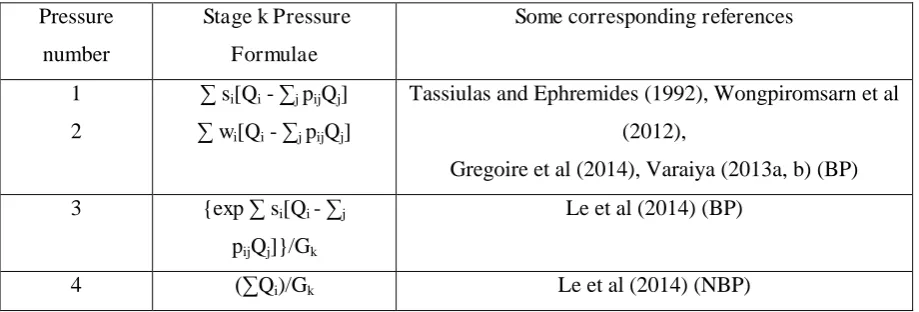
Table 1 gives a list of some reasonable stage pressure formulae and selected relevant papers. Each

sum is over all links i in stage k and pij is the proportion of traffic leaving link i to enter the

downstream link j. The idea of using backpressure (in telecommunication networks) seems to have

first arisen in Tassiulas and Ephremides (1992).

Table 1. Some stage pressure formulae and references where corresponding control policies are considered. The sign “(BP)” means that the relevant stage k pressure formula involves backpressure and the sign “(NBP)” means that the relevant stage pressure does not involve backpressure. .

Pressure

number

Stage k Pressure

Formulae

Some corresponding references

1

2

∑ si[Qi - ∑j pijQj]

∑ wi[Qi - ∑j pijQj]

Tassiulas and Ephremides (1992), Wongpiromsarn et al

(2012),

Gregoire et al (2014), Varaiya (2013a, b) (BP)

3 {exp ∑ si[Qi - ∑j

pijQj]}/Gk

Le et al (2014) (BP)

5 ∑(Qi / gi); ∑(sibi) Smith (1979a, b, c, 1987) (NBP)

6 ∑[Qi - ∑j pijQj] / gi This paper (BP)

7 ∑si[bi - ∑j pijbj] This paper (BP)

The argument in Le et al (2013) appears to apply to show that (under the conditions specified in Le

et. al.) this new P0 backpressure policy 6 stabilises queue lengths if route choices (and so the pij) are

fixed.

5.3.An outline of an extension of assignment – control formulations in sections1-4 into a dynamic

regime using P0

To move the steady state theory in sections 1-4 toward a dynamical theory it is natural to consider

the following dynamic (time-slice) variation of the standard Beckmann et al (1956) objective

function:

V(x, r)











du

u

c

)

(







du

u

f

)

(

Here there are N time slices corresponding to t = 1, 2, 3, . . . , N. Then as in section 4 above, for each

(i, t):

V/xi(t) = ci(xi(t)) + fi (xi(t)+ si ri(t)) and V/ri(t) = si fi (xi(t)+ si ri(t))

and so grad V(x, r) = [c(x) + f(x, r), s•f(x, r)]. This is similar to sections 2-4. To carry through the

theory in sections 2-4 in this dynamic context it is necessary to impose conservation and FIFO

constraints. This is not done here.

6.A modified Varaiya max pressure policy which is not capacity maximising when route choice

is allowed for

The policies and models considered in 6, 7 and 8 below are smooth versions of certain policies

considered in section 5 above; just think of the cycle time being very small, vehicles being very short

and the lost time being zero.

There has recently been a sharp increase in interest in local distributed traffic signal control policies

which are queue stabilising; see for example Varaiya (2013) and Le et al (2013). In almost all of this

work the interaction between these policies and routeing decisions by travellers is not allowed for; and

thus merits attention. In the special network in figure 1 below we consider naturally modified versions

of the Varaiya Max-pressure control policy (called MV here) and the Le et al control policy (called

policy ML here). We show that in this network neither policy MV nor policy ML makes the best of

available network capacity when selfish route choices are allowed for; each policy is sometimes not

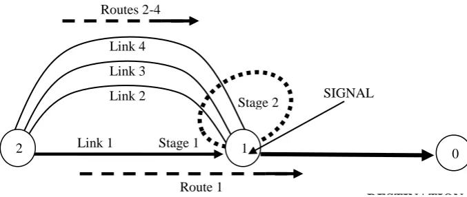
6.1. A network on which neither the MV control policy nor the ML control policy maximizes network

capacity

Figure 1. A four route signalised network; links 2-4 all have exit saturation flow = 1 veh/sec; link 1

has exit saturation flow 2 veh/sec. Stage 1 contains link 1; stage 2 contains links 2-4.

Consider the network in figure 1. Let:

si = the saturation flow at the link i exit (v/sec, for i = 1, 2, 3, 4);

Ci = the freeflow cost/time of travel via routes i = 1, 2, 3, 4 (seconds; constant);

Xi = the flow on route i (veh/sec, for i = 1, 2, 3, 4);

bi = the bottleneck delay at the link i exit (seconds, for i = 1, 2, 3, 4);

Qi = the queue volume on link i (vehicles, for i = 1, 2, 3 and 4);

Gi = the proportion of time that stage i is green (i = 1, 2);

g1 = the proportion of time that link 1 exit is green (equal to G1);

g2 = the proportion of time that link 2 exit is green (equal to G2);

g3 = the proportion of time that link 3 exit is green (equal to G2); and

g4 = the proportion of time that link 4 exit is green (equal to G2).

Suppose that

s1 = 2 and s2 = s3 = s4 = 1

so that the greatest flow is possible when the green-time proportion awarded to stage 2 is as large as

possible. Suppose also that the free-flow travel times Ci along the four routes satisfy

C1 < C2 < C3 < C4.

Of course we impose the natural constraints:

G1 + G2 = 1, G1≥ 0 and G2≥ 0.

But we also here impose a further constraint on G = (G1, G2):

G2≤ 4/7 (or G1≥ 3/7).

This green-time constraint is needed to make the counterexample here work in as simple a way as

possible. However this constraint on G may be very natural in practice. There are two possible

scenarios which might require such a constraint in practice when signal control is being utilised to Link 1 Stage 1

DESTINATION

0

Route 1

SIGNAL Routes 2-4

1 2

Link 2

Stage 2

help with traffic management. First: the green-time constraint G1≥ 3/7 and G2≤ 4/7 may be thought of

as protecting the environment along the three routes 2, 3 and 4, supposing that these three routes pass

through sensitive areas, by disallowing large values of G2. Second: suppose that link 1 is the main

commercial street of a thriving town and the routes 2, 3 and 4 represent different “bypasses”. Then it would be natural to always encourage at least a minimum flow through the town main street for

commercial purposes, and G1≥ 3/7 might be thought of as doing this.

We suppose in this example that T is feasible, bearing in mind the saturation flows and the

green-time constraint. Clearly (given that G1≥ 3/7 and links 2 + 3 + 4 have together a greater saturation flow

than link 1) choosing G = [3/7, 4/7] maximises the green-time allocated to stage 2 and also the

possible OD flow through this network. So

the maximum feasible value of T = the maximum possible throughput = 2.(3/7) + 3.(4/7) =

18/7.

So we also suppose here (for the purposes of this counterexample) that the feasible rigid demand T

(veh/sec.) for travel from the origin to the destination satisfies

2 = 14/7 < T < 18/7;

so that T is feasible (because T < 18/7) but route 1 alone has insufficient capacity for T even if link 1

were given green all the time: because T > 2 the saturation flow of link 1. So if all of the given

demand flow T (veh/sec) does reach the destination then some of that flow must use at least one of the

routes 2-4.

Consider a fixed stage green-time vector G and a corresponding quasi-dynamic equilibrium (x, Q,

b, G). (This is a 4-vector of route flows, a 4-vector of queue volumes, a 4-vector of bottleneck delays

and G, in which flows are all on cheapest routes, unsaturated link exits have zero queue and bi =

Qi/gisi.) We assume that link 5 has a saturation flow > 3 and so is wide enough to accommodate all

possible outflows from links 1-4. We consider these 4-vectors.

We also suppose vertical queueing; so that the cost of traversing route i is Ci + bi. In this paper we

further assume, for each i = 1, 2, 3 and 4, that the queue volume Qi, the bottleneck delay bi and the

link green-time gi are related by:

bi = Qi/gisi. (6.1)

(Of course g1 = G1, g2 = G2, g3 = G2 and g4 = G2.) This formula (6.1) may be motivated in a dynamic

context by assuming that the green-times are slowly varying (in which case (6.1) becomes

approximately true); here however we are assuming that (x, Q, b, G) is a quasi-dynamic equilibrium,

so that (x, Q, b, G) is a constant vector (not varying with time) and in this case (6.1) becomes

accurately true.

Since (x, Q, b, G) is a quasi-dynamic equilibrium, all flow must be on cheapest/quickest routes and

as shown above some flow must use at least one of the routes 2 – 4. Since these routes have a

other routes too) must equilibrate the network. Since C1 < C2 < C3 < C4 these equilibrating bottleneck

delays must thus satisfy:

b4 ≤ b3 ≤ b2 < b1. (6.2)

(At a quasi-dynamic equilibrium the bottleneck delays on shorter routes must compensate exactly for

the longer free-flow travel time of the longest utilised route.)

We will suppose that, in addition to the above conditions which include the quasi-dynamic

user-equilibrium condition, the green times given to stages 1 and 2 are to satisfy a more general dynamic version of Varaiya’s control policy (2013); within this continuous model. We here also assume that link 5 has a very high capacity and that there is zero queue on link 5 so that the backpressure term in

the Varaiya policy is zero.

6.2. A more general dynamic version of the Varaiya Max Pressure signal control Policy

Suppose for the moment now that time is slotted and that all data (on flows, queues and green-times) is available at the time when the “current” time-slot starts. To determine the signal green-times in the “current” time-slot the Varaiya Max Pressure signal control policy on this network utilises Varaiya stage pressures defined as follows:

VP1 = the Varaiya pressure on stage 1 = s1Q1 and (6.3a)

VP2 = the Varaiya pressure on stage 2 = s2Q2 + s3Q3 + s4Q4. (6.3b)

The Varaiya Max Pressure policy then gives all green-time in the “current” short time-slot to the stage

with the greatest pressure at the start time of the current time-slot. If the two stage pressures are both

maximal (and so equal) then resolve the tie arbitrarily.

We modify this policy to the following smoother policy (where we allow all possible proportions of

green-time within a time slot instead of 0 or 1). Suppose given the current queues Q1, Q2, Q3, Q4; these

are the queues at the start of the current time slot. Then the current stage pressures VP1, VP2 are given

by (6.3a) and (6.3b). Suppose given also the previous stage green-time proportions G1, G2; these are

the green-time proportions which were implemented in the previous time slot.

Then the modified Varaiya control policy MV allocates current green-times (to be implemented in

the current time slot) according to the following principle:

MV: given stage green-times in the previous time-slot, each stage green-time can only be reduced

in the current

time slot by swapping some of the previous stage green-time onto currently more pressurised

stages.

The policy of always swapping all green to the most pressurised stage satisfies principle MV, so Varaiya’s original policy satisfies MV. (However green-time allocations arising from principle MV swaps are not necessarily all-or-nothing; so it is more likely that there is quasi-dynamic equilibrium

Definition of an MV green-time equilibrium. If in a time slot no green-time changes are possible

under the defining principle of MV given above, then the distribution of queues and green-times is

said to be an MV green-time equilibrium. An MV equilibrium is thus a triple (X, Q, b, G) such that:

less pressurised stages have no green-time

where the pressures are given by VP1 and VP2.

6.3. Policy MV is inconsistent with quasi-dynamic user equilibrium on some networks.

Under the conditions specified in section 6.2 above, assume now that we are at a quasi-dynamic

equilibrium consistent with MV equilibrium. This is to be

(a) a routeing equilibrium (where all used routes have the same travel time),

(b) an MV equilibrium (as defined above) and (6.4)

(c) a queueing equilibrium (where queues are constant and occur only on saturated links).

(Such an equilibrium is a quasi-dynamic equilibrium [(a) and (c)] consistent with the MV equilibrium

condition (b).) At such a consistent equilibrium there is no incentive for route flows, green-times or

queue lengths to change.

Here (in our continuous context) we now show that (6.4) is impossible on this network shown in

figure 1; even though the demand T (which satisfies 2 = 14/7 < T < 18/7) is within the network

capacity.

So assume that 2 = 14/7 < T < 18/7 and that (6.4) holds at (X, Q, b, G). As we are at a user

equilibrium and (6.1) holds it follows that (6.2) also holds and so

Q4 / s4g4 ≤ Q3 /s3 g3≤ Q2 /s2g2 < Q1 / s1g1.

Then, using the given saturation flows and the stage green-times,

Q4 / G2≤ Q3 / G2≤ Q2 / G2 < Q1 / 2G1.

So

Q4 ≤ Q3 ≤ Q2 < (Q1 / 2)(G2 / G1)

This line above yields the following three inequalities:

Q4 < (Q1/2)(G2/G1);

Q3 < (Q1/2)(G2/G1); and

Q2 < (Q1/2)(G2/G1).

Adding the three inequalities:

Q4 + Q3 + Q2 < 3(Q1/2)(G2/G1).

Thus, since s1 = 2, s2 = s3 = s4 = 1 and G2 / G1≤ 4/3 (this is the green-time constraint we are imposing),

s4Q4 + s3Q3 + s2Q2 < (3/2)(s1Q1/2)(G2/G1) = (3/4)(s1Q1)(G2/G1) ≤ (3/4)(s1Q1)(4/3) = s1Q1.

It follows that at any user equilibrium and at any green-time vector G (satisfying the green-time

constraint):

It now follows that, at an MV equilibrium green-time, the stage 2 green-time = 0 and the stage 1

green-time = 1. But T > 14/7 = 2 (the saturation flow of link 1); and so the inflow T exceeds the

maximum possible outflow of link 2 and the queue on link 1 cannot be constant.

Thus the any feasible demand T satisfying 2 = 14/7 < T < 18/7 cannot be satisfied at a

quasi-dynamic equilibrium when the MV policy is followed. (A slow quasi-dynamical model will have unbounded

queues.)

7. A modified Le et al signal control policy which is not capacity maximising when route choice

is allowed for

7.1. The Le et. al. signal control policy may not be consistent with quasi-dynamic user equilibrium.

A similar analysis to that given above may be applied to a signal control policy designed by Le et al

(2013), with no modification; still using the network in figure 1. In this section the definitions and

constraints in section (6.1) all hold including the added green-time constraint G1 ≥ 3/7. One difference

now is that time slots are replaced by “proper” signal cycles.

Stage pressures are also defined very differently by Le et al (2013) who start with stage weights as

follows:

Le et al stage 2 weight = exp(s2Q2 + s3Q3 + s4Q4) and

Le et al stage 1 weight = exp(s1Q1).

Then, given the values of these weights in a current cycle, Le et al (2013) suggest making the stage

green-times during the next cycle proportional to these weights; or

G1 = exp(s1Q1)/[exp(s2Q2 + s3Q3 + s4Q4) + exp(s1Q1)]

and

G2 = exp(s2Q2 + s3Q3 + s4Q4)/[exp(s2Q2 + s3Q3 + s4Q4) + exp(s1Q1)]

Such a green-time vector G equalises the two Le et al stage pressures given below:

LP1 = Le et al stage 1 pressure = exp(s1Q1)/G1;

LP2 = Le et al stage 2 pressure = exp(s2Q2+ s3Q3+ s4Q4)/G2.

Here we show that for a range of feasible demands T this policy is inconsistent with quasi-dynamic

equilibrium on the network in figure 1, by using arguments very similar to those given above in the

Varaiya case.

Suppose we are at a quasi-dynamic user equilibrium so that (6.1) and (6.2) both hold. Then as

shown above in the Varaiya case (using (6.1), (6.2) and the green-time constraint G1≥ 3/7):

s4Q4 + s3Q3 + s2Q2 < s1Q1.

It follows immediately that (at a quasi-dynamic user equilibrium)

exp(s4Q4 + s3Q3 + s2Q2) < exp(s1Q1)