Comparisons between different techniques for measuring mass segregation

mass segregation

.

White Rose Research Online URL for this paper:

http://eprints.whiterose.ac.uk/85726/

Version: Accepted Version

Article:

Parker, R.J. and Goodwin, S.P. (2015) Comparisons between different techniques for

measuring mass segregation. Monthly Notices of the Royal Astronomical Society, 449 (4).

pp. 3381-3392. ISSN 0035-8711

https://doi.org/10.1093/mnras/stv539

eprints@whiterose.ac.uk

https://eprints.whiterose.ac.uk/

Reuse

Unless indicated otherwise, fulltext items are protected by copyright with all rights reserved. The copyright

exception in section 29 of the Copyright, Designs and Patents Act 1988 allows the making of a single copy

solely for the purpose of non-commercial research or private study within the limits of fair dealing. The

publisher or other rights-holder may allow further reproduction and re-use of this version - refer to the White

Rose Research Online record for this item. Where records identify the publisher as the copyright holder,

users can verify any specific terms of use on the publisher’s website.

Takedown

If you consider content in White Rose Research Online to be in breach of UK law, please notify us by

arXiv:1503.02692v1 [astro-ph.GA] 9 Mar 2015

Comparisons between different techniques for measuring

mass segregation

Richard J. Parker

_{and Simon P. Goodwin}

1_{Astrophysics Research Institute, Liverpool John Moores University, 146 Brownlow Hill, Liverpool, L3 5RF, UK} 2_{Department of Physics and Astronomy, University of Sheffield, Sheffield, S3 7RH, UK}

11 March 2015

ABSTRACT

We examine the performance of four different methods which are used to measure mass segregation in star-forming regions: the radial variation of the mass function

M_{MF; the minimum spanning tree-based ΛMSR method; the local surface density}

ΣLDRmethod; and the ΩGSRtechnique, which isolates groups of stars and determines

whether the most massive star in each group is more centrally concentrated than the average star. All four methods have been proposed in the literature as techniques for quantifying mass segregation, yet they routinely produce contradictory results as they do not all measure the same thing. We apply each method to synthetic star-forming regions to determine when and why they have shortcomings. When a star-forming region is smooth and centrally concentrated, all four methods correctly identify mass segregation when it is present. However, if the region is spatially substructured, the ΩGSR method fails because it arbitrarily defines groups in the hierarchical

distribu-tion, and usually discards positional information for many of the most massive stars in the region. We also show that the ΛMSR and ΣLDR methods can sometimes

pro-duce apparently contradictory results, because they use different definitions of mass segregation. We conclude that only ΛMSR measures mass segregation in the classical

sense (without the need for defining the centre of the region), although ΣLDR does

place limits on the amount of previous dynamical evolution in a star-forming region.

Key words: stars: formation – star clusters: general

1 INTRODUCTION

Most young (<10 Myr) stars are observed in the company of others, either in clusters (Lada & Lada 2003), groups (Porras et al. 2003), associations (Blaauw 1964) or in re-gions which are over-dense with respect to the Galactic field (Bressert et al. 2010). Attempts have been made at distin-guishing isolated versus clustered star-formation, or clus-ters versus associations (e.g. Cartwright & Whitworth 2004; Gieles & Portegies Zwart 2011). However, it appears that (at least on local scales) there is no fundamental scale unit for star formation (e.g. Bressert et al. 2010), and that clus-ters may just be the dense tail of the distribution of Galactic star formation (Kruijssen 2012).

Given that star formation on pc-scales often seems to produce complex, hierarchical distributions, it is crucial to be able to examine the spatial distributions of stars in a quantitative, statistical way. This allows us to extract infor-mation on star forinfor-mation and compare and contrast different regions (and simulations). One such indicator is the relative

⋆ _{E-mail: R.J.Parker@ljmu.ac.uk}

positions of the most massive stars with respect to the aver-age stars in a region – often referred to as ‘mass segregation’ when the most massive stars are more centrally concentrated than average.

In recent years several alternative methods for measur-ing mass segregation have been proposed in the literature. In this paper we critically assess several of the new methods, including the ΛMSRmethod (Allison et al. 2009), the Σ−m or ΣLDRmethod (Maschberger & Clarke 2011) and the tech-nique of dividing a star-forming region into groups to deter-mine the relative distance of the most massive star to the centre of each group (Kirk & Myers 2011; Kirk et al. 2014), which we call ΩGSR. A similar study to compare mass segre-gation methods was previously carried out by Olczak et al. (2011); however, the ΣLDRand ΩGSR methods were not yet prominent in the literature and therefore not included in that study. A full appraisal of these methods – and ΛMSR– using synthetic data is therefore required in order to make sense of the growing literature in this area.

paper in detail. In Section 3 we test these methods on syn-thetic data, before discussing our results in Section 4 and concluding in Section 5.

2 WHAT IS MASS SEGREGATION?

‘Mass segregation’ is a phrase often used in relation to star clusters and regions, but often it is not defined.

The classical definition of mass segregation is based on the behaviour of dynamically old bound systems (i.e. relaxed and virialised star clusters). The process of two-body relax-ation redistributes energy between stars and they approach energy equipartition whereby all stars have the same mean kinetic energy – this means that more massive stars will have a velocity dispersion that is lower. Because the velocity dis-persion of the more massive stars is lower, they will tend to be concentrated towards the centre of the cluster (Spitzer 1969).

The timescale,tMS(M), on which stars of massM will dynamically mass segregate depends on the mean mass of stars hmi and the two-body relaxation time,trelax(Spitzer 1969)

tMS(M)∼ M

hmitrelax. (1)

Therefore in old star clusters (especially globular clusters) we expect to see mass segregation down to low masses and that mass segregation is explicable entirely by dynamics.

In these old clusters, the two-body dynamics that may have caused any mass segregation will also remove any primordial substructure in the spatial distribution and we would expect (and observe) the cluster to have a smooth, centrally concentrated spatial distribution, such as a Plummer (1911) or King (1966) profile.

In this case, the clusters have a well-defined radial pro-file where one can quantify mass segregation by taking dif-ferent mass bins and comparing the density profiles (e.g. Hillenbrand 1997; Pinfield et al. 1998), or examining varia-tions in the slope of the mass function (or luminosity func-tion) with distance from the cluster centre (Carpenter et al. 1997; de Grijs et al. 2002; Gouliermis et al. 2004). A related method is to quantify the variation of the ‘Spitzer radius’ – the rms distance of stars in a cluster around the centre of mass – with luminosity (Gouliermis et al. 2009).

The motivation in attempting to observe mass segrega-tion in young clusters or regions is that it might not have a dynamical origin. If we observe mass segregation in a region that is so young that two-body encounters cannot have mass segregated the stars1, then the mass segregation must be set by some aspect of the star formation process, and is often labelled ‘primordial mass segregation’.

Primordial mass segregation has been found in some simulations of star formation (e.g. Maschberger & Clarke 2011; Myers et al. 2014) but not in others (Girichidis et al. 2012; Parker et al. 2015), and we also note that any ob-served signature may be a combination of primordial and dynamical mass segregation (Moeckel & Bonnell 2009), and

1 _{This is complicated by the fact that it is not the current}

re-laxation time of the region that is important, rather it is how dynamically old the region is (see Allison et al. 2010).

to complicate matters further mass segregation can be intro-duced very rapidly dynamically through violent relaxation rather than two-body relaxation (see Allison et al. 2010).

Observationally, mass segregation has been searched for in clusters and star forming regions for many years (e.g. Sagar et al. 1988; de Marchi & Paresce 1996; Hillenbrand & Hartmann 1998; Raboud & Mermilliod 1998; de Grijs et al. 2002; Gouliermis et al. 2004; Sabbi et al. 2008; Gouliermis et al. 2009, and many more), but in the past few years a number of new statistical methods have been developed for finding mass segregation, and the pur-pose of this paper is to examine whatexactlythey are search-ing for, and what problems they might have.

Here we briefly describe the most commonly used meth-ods and their assumptions. In the next section we describe exactly how we implement each method in detail.

It should be noted that all methods suffer from a poten-tially very serious problem. All methods examine the relative distributions of high- and low-mass stars. Therefore the dis-tribution of low-mass stars must be known, however these are very faint compared to the high-mass stars in young re-gions/clusters. And so the location in which the observer is biased against observing low-mass stars is near luminous high-mass stars which is exactly where one needs to know if low-mass stars are present or not. In this paper we use fake data in which we have the advantage of knowing exactly where every star is and what its mass is, but real obser-vations do not have this advantage (see Stolte et al. 2005; Ascenso et al. 2009, for a detailed discussion of observational selection effects and biases).

2.1 Radial mass functions,MMF

Until recently, the most commonly used way of determining mass segregation was to compare the radial distribution of the mass function, or the radial distribution of stars of dif-ferent masses (e.g. Sagar et al. 1988; Gouliermis et al. 2004; Stolte et al. 2006; Sabbi et al. 2008; Chavarr´ıa et al. 2010). In this definition, if a cluster is mass segregated the most massive stars are preferentially towards the centre, and low-mass stars preferentially in the outskirts. Therefore the slope of the mass function should be flatter in the centre than the outskirts, and/or the low-mass stars should have a much broader radial distribution.

This method suffers three significant drawbacks. One is that it requires a ‘centre’ to be defined. In relaxed, virialised star clusters there is a centre from which this can be mea-sured, but in substructured and messy young star forming regions it is unclear if defining a ‘centre’ means anything at all, and even if it did, it is unclear how one would practically do this. One can define a geometric centre based on the po-sitions of stars, but in some morphologies (as we shall see) this ‘centre’ is not near to, nor is the central location, of the stars.

Second, the definition of radial bins is non-trivial and often arbitrary, which adds a further level of complexity to the interpretation of any signal.

It also suffers from poor statistics, in that it is unclear how to compare different clusters or provide anyquantitative

information on the mass segregation.

distribution of the radii of all the stars in the distribution. We set the ‘centre’ of the region to be the (known to us) centre of mass of the region. We gauge the significance of any difference using a Kolmogorov-Smirnov (KS) test, and rather generously use a p-value of<0.1 as our significance threshold.

2.2 The ΛMSR-parameter

In order to try and avoid the problems of defining a centre and to produce a quantitative statistic to aid comparisons Allison et al. (2009) introduced the ΛMSR-parameter.

The ΛMSR-parameter examines the relative (2D) spatial distributions of the N most massive stars relative to each-other with the spatial distributions ofNrandom stars. This is done by finding the edge length of the minimum spanning tree (MST) that connects the N most massive stars with many MSTs ofN random stars.

This has the great advantage that it does not require a centre or any special position to be defined. It also produces a number with associated error that states how much longer or shorter the massive star MST is compared to random MSTs, and how likely it is that this length could be drawn at random from the random MSTs (i.e. how likely is this to occur by random chance).

The ΛMSR-parameter measures a very similar ‘mass seg-regation’ to the classical definition: it examines if the mas-sive stars are closer to each-other than one would expect by random chance. If the massive stars are closer to one another, then the star-forming region is said to be mass seg-regated.

It practice, we take the ratio of the average (mean) ran-dom MST length to the subset MST length, a quantitative measure of the degree of mass segregation (normal or in-verse) can be obtained. We first determine the subset MST length,lsubset. We then determine the average length of sets of NMSTrandom stars each time, hlaveragei. There is a dis-persion associated with the average length of random MSTs, which is roughly Gaussian and can be quantified as the stan-dard deviation of the lengthshlaveragei ±σaverage. However, we conservatively estimate the lower (upper) uncertainty as the MST length which lies 1/6 (5/6) of the way through an ordered list of all the random lengths (corresponding to a 66 per cent deviation from the median value, hlaveragei). This determination prevents a single outlying object from heav-ily influencing the uncertainty. We can now define the ‘mass segregation ratio’ (ΛMSR) as the ratio between the average random MST pathlength and that of a chosen subset, or mass range of objects:

ΛMSR=

hlaveragei

lsubset

+σ5/6/lsubset

−σ1/6/lsubset

. (2)

A ΛMSRof∼1 shows that the stars in the chosen subset are distributed in the same way as all the other stars, whereas ΛMSR >1 indicates mass segregation and ΛMSR <1 indi-cates inverse mass segregation, i.e. the chosen subset is more widely distributed than the other stars.

Note that a slightly different formulation of ΛMSR, which uses the geometric mean to define the uncertainties, is available (Olczak et al. 2011), but for the purposes of this paper the original method by Allison et al. (2009) is suffi-cient.

2.3 The local density ratio,ΣLDR

Maschberger & Clarke (2011) introduced another measure of mass segregation – the local density ratio. For this the local surface density of every star Σ is found, and the average local surface density of theNmost massive stars is compared to the average local surface density of all stars to obtain the ‘local surface density ratio’, ΣLDR(K¨upper et al. 2011; Parker et al. 2014). This is able to determine if the most massive stars are in regions of significantly higher (or lower) local surface density than would be expected by random chance. If the most massive stars are in areas of higher local density than the region average, the region is said to be mass segregated.

As with ΛMSR, ΣLDRmakes no assumptions about there being a centre. However it is possible that the same numeri-cal value of ΣLDRcan be statistically significant sometimes, but not other times, which we quantify by means of a KS test.

It is very important to note that ΛMSRand ΣLDR mea-sure different versions of ‘mass segregation’. ΛMSR deter-mines if the massive stars are closer to each other than one would expect by random chance, ΣLDR determines if the massive stars are in regions of higher surface density than one would expect by random chance.

It would be quite possible for ΣLDRto find ‘mass segre-gation’, but for ΛMSRnot to. This would occur for example if the massive stars were widely distributed, but each had a local overdensity of low-mass stars (see Parker et al. 2014, for examples).

In practice, we calculate the local stellar surface den-sity following the prescription of Casertano & Hut (1985), modified to account for the analysis in projection. For an individual star the local stellar surface density is given by

Σ =n−1 πr2

n

, (3)

where rn is the distance to the nth nearest neighbouring

star2_.

K¨upper et al. (2011) and Parker et al. (2014) took the ratio of the median surface density of a chosen subset (in this paper we will use the 10 most massive stars) to the median for all stars in a region to define the local surface density ratio, ΣLDR:

ΣLDR= ˜ Σsubset

˜ Σall

. (4)

The ΣLDR ratio is then quoted with the p-value from the KS test to gauge the significance of any deviation from the median for all stars, again with ap-value<0.1 used as the boundary between the difference being significant or not.

2.4 Group segregation ratio,ΩGSR

A further, alternative method for quantifying mass segre-gation was recently suggested by Kirk & Myers (2011) and Kirk et al. (2014). In this method stellar groups are identi-fied and ‘isolated’ from the total distribution. Each of these

groups is then examined to see if the most massive star it contains is closer to the centre of the group than the median distance of all stars in the group. If the most massive star is closer to the centre than the average star in the major-ity of the groups, the star-forming region is said to be mass segregated.

The ‘mass segregation’ searched for in this method is different again from both ΛMSR and ΣLDR. ΩGSR divides the region into groups and then examines each group for evidence of internal mass segregation. In this process many stars in the region (possibly including some of the most mas-sive) can be excluded if they do not belong in a group.

First, an MST is constructed for the entire region and a cumulative distribution of all MST branch lengths is then made. Two power-law slopes are then fitted to the short-est lengths, and the longshort-est lengths, and the intersection of these slopes defines the boundary of subclustering, dbreak (Gutermuth et al. 2009).

The links in the full MST which exceed dbreak are re-moved, resulting in the star-forming region being divided into groups. If the position of the most massive star in the grouprmmis closer to the central position than the median value for all stars,rmed, the group, or subcluster has an off-set ratio (rmm/rmed) less than unity and is said to be mass segregated.

In this paper, we define a ‘group segregation ratio’, ΩGSR, as

ΩGSR=

Nseg

Ngrp

, (5)

whereNgrpare the number of groups, andNsegis the number of these groups that have an offset ratio less than unity. If a star-forming region has ΩGSR= 1, then all individual groups defined bydbreak are mass segregated.

It should be noted that, just by random chance we would expect ΩGSR∼0.5, as half of the time the most mas-sive star would be in the inner 50 per cent of stars. The significance of ΩGSR ∼0.5 is affected by Poisson noise; for example an ΩGSR= 0.8 is not significant if it is 8 out of 10 subgroups.

3 FINDING MASS SEGREGATION IN

SIMULATED REGIONS

All of these four methods for finding ‘mass segregation’ will find classical mass segregation in a relaxed, spatially smooth, spherical, bound cluster. If the most massive stars are close together in the centre of a spherical cluster then: (A)MMF will show a different mass function in the inner regions. (B) ΛMSRwill show that the massive stars are concentrated to-gether. (C) ΣLDRwill find that the most massive stars are in the regions of highest surface density. (D) ΩGSR will find that the most massive star is towards the centre of a single group (in this situation, the cluster itself is the group).

In such a situation we would advise the reader to use ΛMSRto look for mass segregation as it gives a single quanti-tative value for the degree of mass segregation with an asso-ciated error, and can easily determine the stellar mass down to which mass mass segregation is present (e.g. Allison et al. 2009; Sana et al. 2010; Beccari et al. 2012; Delgado et al.

2013; Er et al. 2013; Pang et al. 2013; Rivilla et al. 2014; Wright et al. 2014).

What we will examine in this paper is the analysis of complex, substructured regions and the search for ‘mass seg-regation’ within them, according to the definition presented in each method.

In this Section we run our four methods for quanti-fying mass segregation on a synthetic dataset containing N = 300 stars to match the small-N statistics of many young regions. We distribute the stars in a fractal distribu-tion according to the prescripdistribu-tion in Goodwin & Whitworth (2004), Allison et al. (2010) and Parker et al. (2014). We refer the reader to those papers for a detailed description of how the fractal is set up, but we briefly summarise the method here. The fractal is built by creating a cube con-taining ‘parents’, which spawn a number of ‘children’ de-pending on the desired fractal dimension, D. The amount of substructure is then set by the number of children that are allowed to mature (the lower the fractal dimension, the fewer children mature and the cube has more substructure). We choose a fractal distribution because the ΛMSR, ΣLDR and ΩGSR methods were developed specifically to be used on substructured, or hierarchical spatial distribu-tions of stars in star-forming regions and clusters. All three negate the requirement of designating a ‘centre’ (although the ΩGSR method requires the definition of group centres – as detailed in Section 2.4). Star-formation may result in a truly fractal distribution (Elmegreen & Elmegreen 2001; Cartwright & Whitworth 2004), but star forming regions are unlikely to retain their primordial spatial distribution due to dynamical evolution (Parker et al. 2014). As a default, we chooseD= 2.0 and assign the fractal a radius of 5 pc.

We note that observed star-forming regions display a range of fractal dimensions (Cartwright & Whitworth 2004; Schmeja et al. 2008, 2009; S´anchez & Alfaro 2009; Gouliermis et al. 2014). It is possible that all regions may form with the same (low) fractal dimension, and ob-served differences are due to differing amounts of dynamical evolution (Goodwin & Whitworth 2004; Parker et al. 2014; Parker 2014), although simulations of star-formation also produce a range of values before significant dynamical evo-lution takes place (Girichidis et al. 2012; Dale et al. 2012, 2013). For the purposes of the numerical tests presented here, regions withD= 2.0 adequately highlight the differ-ences between the various definitions of mass segregation.

We draw masses from the Maschberger (2013) formula-tion of the initial mass funcformula-tion (IMF):

p(m)∝

m µ −α 1 + m µ

1−α!−β

. (6)

Eq. 6 essentially combines the log-normal approximation for the IMF derived by Chabrier (2003, 2005) with the Salpeter (1955) power-law slope for stars with mass>1 M⊙.

Here, µ = 0.2 M⊙ is the average stellar mass, α = 2.3

is the Salpeter power-law exponent for higher mass stars, and β = 1.4 is the power-law exponent to describe the slope of the IMF for low-mass objects (which also deviates from the log-normal form; Bastian, Covey & Meyer 2010). Finally, we sample from this IMF within the mass range mlow= 0.01 M⊙tomup= 50 M⊙.

distri-bution is unimportant, because we are comparing the posi-tions of the 10 most massive stars to the posiposi-tions of all stars in a region. In this case, we only require the massive stars to have masses above those of the remaining 290 objects.

However, stochastic sampling of the IMF for low-N re-gions can result in very different mass distributions between realisations (Parker & Goodwin 2007), and if we were to study the subsequent dynamical evolution, differences in the relative masses of individual stars could affect the measured amount of mass segregation.

We created 20 realisations of the fractal distribution (and mass distribution). However, in the following we con-centrate on just one typical realisation of the spatial dis-tribution, and mass distribution of stars. The realisation is ‘typical’ in the sense that it nicely highlights the advantages, and disadvantages of each of the methods.

For each realisation we assign the stellar masses in one of three ways. First the stellar masses are randomly assigned, so no mass segregation – whatever the definition – should be detected (Section 3.1). We then change the positions of the ten most massive stars so that they are either more centrally concentrated (Section 3.2) or in the locations of the highest stellar surface density (Section 3.3).

We perform all the subsequent analysis in 2 dimensions in order to mimic the information available to observers.

It should be noted thatallmethods make a hidden as-sumption that the 2 dimensional distributions are a good representation of the true 3 dimensional structure (in the sense that they retain the same information on spatial dis-tributions). It is unclear if this is really the case, and we will return to this difficult question in a later paper. For now we will proceed under the assumption that the 2 dimensional distributions do retain the important information present in the true 3 dimensional structure.

3.1 Random distributions of stellar masses

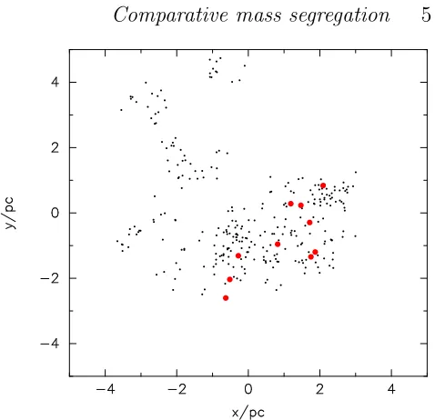
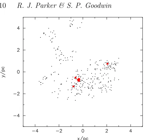
In this section we use our four techniques for measuring mass segregation on a random distribution of stars, as shown in Fig. 1. The locations of the ten most massive stars are shown by the large red dots.

3.1.1 Radial mass functions,MMF

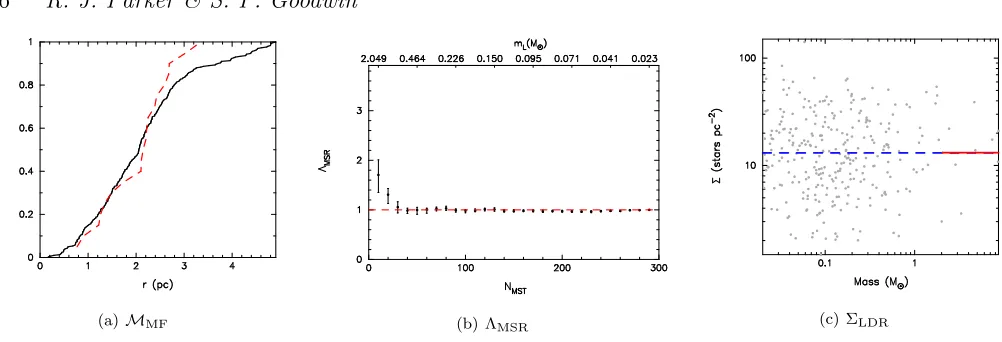
In Fig. 2(a) we show the cumulative distribution of the ra-dial distances from the centre of the fractal for all stars (the solid black line) and for the ten most massive stars (the red dashed line). Within 3 pc of the centre, the two distribu-tions are overlaid. However, there are no massive stars at radii greater than 3.2 pc and the cumulative distributions differ beyond this radius. However, a KS test on the two distributions returns ap-value of 0.51 that the two popula-tions share the same parent distribution, i.e. the difference is not significant in that it is higher than our threshold of p= 0.1.

It is important to note that the centre of the distribution is known to us to be at{0,0}pc. When confronted with a distribution similar to that shown in Fig. 1, an observer would use the average position of all the stars to define a centre. In the example shown here, this average position is almost identical to the centre of mass.

Figure 1.A fractal distribution (D= 2.0) with stars randomly drawn from an initial mass function and placed randomly in the spatial distribution. The ten most massive stars are shown by the larger (red) points.

3.1.2 Mass segregation ratio, ΛMSR

In Fig. 2(b) we show ΛMSRas a function of theNMSTstars for the fractal region in Fig 1. ΛMSR = 1 (consistent with there being no mass segregation) is shown by the horizon-tal red dashed line. The ΛMSRtechnique shows that the 10 most massive stars are slightly more centrally concentrated than the average stars, with ΛMSR= 1.7+0−0..34 for stars with

m >2.05. The 20 most massive stars are also slightly more centrally concentrated than the average stars.

This positive signal of mass segregation is likely due to the same spatial feature in Fig. 1 that shows an apparent difference in the radial mass functions, namely that none of the most massive stars are more than 3 pc from the centre (Fig. 2(a)). This is a 2-σdifference from unity, and so would be expected roughly 1-in-20 times. By ‘fluke’ this is the only random realisation that shows a 2-σ signature of mass seg-regation and emphasises the need to avoid over-interpreting a single 2-σresult.

3.1.3 Local density ratio,ΣLDR

In Fig. 2(c) we plot the local stellar surface density, Σ, against individual stellar mass m in Fig. 2(c). The me-dian stellar surface density for the entire distribution is 13.1 stars pc−2 _{(the blue dashed line) whereas the median} stellar surface density for the ten most massive stars is 13.2 stars pc−2

(a)MMF (b) ΛMSR (c) ΣLDR

Figure 2.Three separate measures of mass segregation for the stellar distribution shown in Fig. 1. In panel (a) we show the cumulative distribution of the distance from the centre for the ten most massive stars (the red dashed line) and the cumulative distribution for all stars (the solid black line) – the mass function comparison,MMF. In panel (b) we show the ΛMSRmass segregation ratio as a function of

theNMSTstars used in the subset (the lowest mass star,mL, for variousNMSTvalues is shown along the top horizontal axis). ΛMSR= 1

(i.e. no preferred spatial distribution) is shown by the solid horizontal red dashed line. In panel (c) we show local stellar surface density versus stellar mass (the Σ−mplot). The median stellar surface density for the ten most massive stars is shown by the righthand solid (red) horizontal line and the median surface density for all of the stars is shown by the blue horizontal dashed line.

3.1.4 Group segregation ratio,ΩGSR

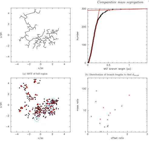
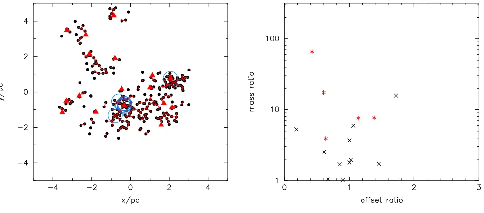
In Fig. 3 we show the determination of the ΩGSR group segregation ratio. We start by constructing an MST of the entire region, as shown in Fig. 3(a). The cumulative dis-tribution of the branches in the entire MST is shown in Fig. 3(b), and the two power law fits to the close branches and the long branches are shown by the solid red lines. Fol-lowing Gutermuth et al. (2009); Kirk & Myers (2011) and Kirk et al. (2014) we take the intersection of these lines as the MST dbreak = 0.28 pc, the boundary between ‘clus-tered’ and ‘diffusely’ distributed stars. All MST branches with length< dbreak are retained (Fig. 3(c)) which defines groups within the distribution3_.

In Fig. 3(c) we show the groups (withN >2) selected by this method as the stars still connected by the red MST links. The most massive star within each of the groups is marked by a red triangle. The ten most massive stars in the entire region are shown by the large open blue circles.

It might be considered thatdbreak= 0.28 pc has a physi-cal importance – it is the apparent break between structures. However, in this simulation this distance has no physical significance, it is just a projected 5 pc radiusD= 2.0 box fractal distribution, which by design is hierarchical and self-similar, with no special spatial scale (apart from the radius itself). Examination of Fig. 3 shows that there is nothing ‘special’ about this distance. Furthermore, small changes to dbreak can drastically affect the number of groups which are identified. For example, if we choose dbreak = 0.25 pc (the point at which the cumulative distribution in Fig. 3(b) de-viates from the steep power-law), we identify 18 groups (in-stead of the 16 identified using dbreak = 0.28 pc). If we choose dbreak = 0.5 pc (where the shallow power-law slope deviates from the tail of the distribution), we identify only 6 groups.

3 _{Other methods to define groups/clusters in crowded fields may}

have advantages over the MST technique – see Schmeja (2011) for a review.

Examination of Fig. 1 shows to the eye perhaps five groups, the most significant being to the bottom right. Fig. 3(c) shows that ΩGSRhas identified many more groups than this. In particular, the stars to the bottom left (around {−3,−1}pc) have been split into three groups. And the sig-nificant distribution of stars at the bottom centre/right have been split into several groups, but some stars (including one of the most massive in the region) have not been included in any group.

The identification of groups is crucial to the ΩGSR method, but it is unclear from Fig. 3(c) that the selected groups are ‘real’ in any sense.

There are three other significant issues with the ΩGSR method that are immediately apparent from Fig. 3(c).

Firstly, the most massive star in a group may not be one of the most massive stars in the region. All of the groups to the upper left have a locally most massive star that is not one of the most massive stars in the region as a whole.

Secondly, a group may contain more than one of the truly most massive stars in a region (e.g. three of the larger groups to the bottom right) in which case only the most massive of these is considered and the other (truly massive for the region) stars are discarded.

Thirdly, if a truly massive star is not part of a group (surely an interesting phenonena) then it is discarded from the analysis entirely (e.g. the large open blue circle at the bottom centre).

(a) MST of full region _{(b) Distribution of branch lengths to findd}

break

(c) Groups identified by MSTdbreak (d) Mass ratio versus position offset ratio for groups

Figure 3.Mass segregation as defined by the ΩGSR method. In panel (a) an MST of the full spatial distribution is shown, and the

cumulative distribution of all of the branch lengths is shown in panel (b). The two power law slopes used to fit the data are shown by the red lines. The intersection of these slopes gives the critical MST length,dbreak, and in panel (c) we show the groups identified using

this length. In the groups in which there are 3 or more stars the most massive star in the group is shown by the solid red triangle. The positions of the ten most massive stars in thefull distribution are shown by the large open blue circles (these correspond to the filled red circles in Fig. 1). In panel (d) we show the mass ratio of the most massive star in each group to the group median mass versus the ratio of the position of the most massive star to the median position of the group. Groups with ten or more stars are shown by the red asterisks.

with N > 2, ΩGSR = 0.59 and for groups with N > 10, ΩGSR= 0.604. In a truly random distribution, ΩGSR= 0.5. It is worth noting another problem here, in that the ΩGSR method needs to define a ‘centre’ of each group from which to measure distances. Therefore there is an implicit

4 _{Note that Kirk & Myers (2011) and Kirk et al. (2014) generally}

only present statistics for groups containing 10 or more stars, and we will also draw conclusions based only on these ‘large’ groups.

assumption of spherical symmetry which examination of Fig. 3(c) shows not to be the case in most groups.

ac-Figure 4.As Fig. 1; a fractal distribution of stellar masses ran-domly drawn from an initial mass function. However, in this case we have swapped the locations of the ten most massive stars (shown by the larger red points) with the ten most central stars.

cording to this method). Again, both ΛMSR and ΣLDR are consistent with no mass segregation (normal or inverse).

3.2 Massive stars centrally concentrated

We now swap the positions of the 10 most massive stars with the positions of the 10 stars closest to the centre of the fractal distribution, as shown by the red points in Fig. 4. This is clearly a rather artificial distribution of the most massive stars, but it is one that most closely matches the ‘classical’ definition of mass segregation for this region.

3.2.1 Radial mass functions,MMF

In Fig. 5(a) the cumulative distribution of radial positions of the 10 most massive stars is shown by the red dashed line, whereas the cumulative distribution of the radial positions for all stars is shown by the solid black line. Due to the central concentration of the most massive stars, the KS test returns ap-value of 2×10−4 _{that the two subsets share the} same parent distribution.

This result demonstrates that if we have confidence in the definition of the centre of a region, a strong mass seg-regation signature may still be seen in substructured distri-butions using the radial mass function technique.

3.2.2 Mass segregation ratio,ΛMSR

We show the ΛMSR ratio in Fig. 5(b). The ten most mas-sive stars have ΛMSR= 5.3+0−1..90, which is significantly above unity. In 20 realisations, only 1 star-forming region displays a ΛMSRratio that is not significantly above unity, with val-ues ranging from ΛMSR= 2.0+0−0..34 to ΛMSR= 11.1+1−1..14.

This is completely unsurprising as ΛMSR is designed to measure exactly this type of mass segregation – the most massive stars being much closer to one-another than a ran-dom sample of stars would be.

3.2.3 Local density ratio,ΣLDR

Interestingly, the ΣLDRratio does not reflect the central con-centration of the 10 most massive stars. ΣLDR= 0.58 due to the most centrally located stars being in areas of relatively low surface density, although a KS test returns a p-value of 0.26 that the massive stars have a different parent dis-tribution to the full disdis-tribution (i.e. this difference is not significant). That said, most people would conclude simply from eye that the distribution shown in Fig. 4 is mass segre-gated, even though the massive stars have low local surface density. In 20 realisations of this distribution, ΣLDR does not detect mass segregation in 11, and in a further 5 it finds inverse mass segregation.

3.2.4 Group segregation ratio,ΩGSR

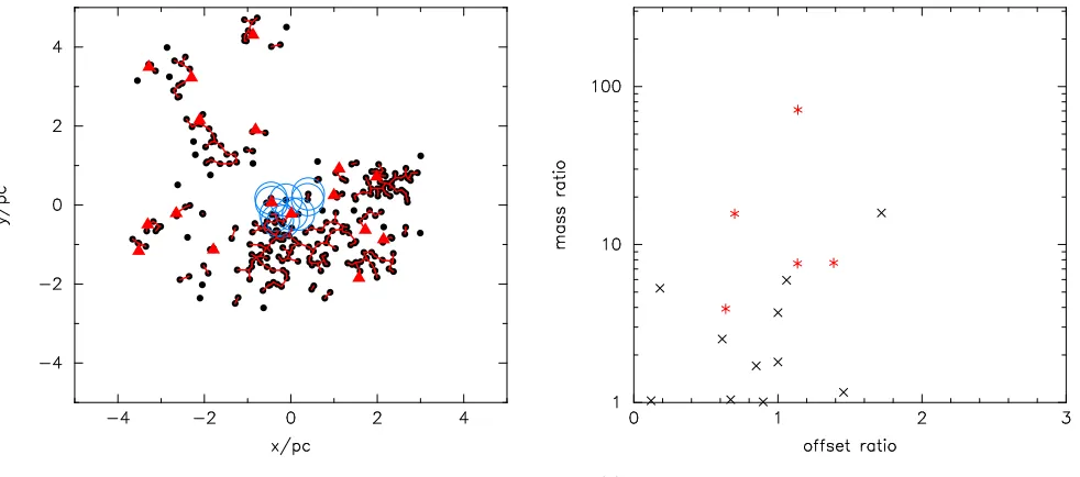
The overall spatial distribution has not changed between Figs. 1 and 4 and so the determination of dbreak and the subsequent identification of groups is identical to that in Sec-tion 3.1. We show the groups defined bydbreak in Fig. 6(a), noting the change of location of the 10 most massive stars in the full distribution (the blue open circles). The locations of the most massive star in each group (shown by the red triangles) have also changed in some cases.

Again, we note that two of the 10 most massive stars from the full distribution are now no longer part of a group with N > 2, and instead are in a pair (located at {0.4,0.1}pc). We show the mass ratio versus offset ratio for all groups with N > 2 stars in Fig. 6(b). Again, the five groups with N > 10 stars are shown by the red points. This time only two of these five groups are mass segregated (ΩGSR= 0.40), even though the global distribution of mas-sive stars is very mass segregated.

In this situation – where the most massive stars in a region are ‘centrally’ concentrated, it is not clear what ΩGSR is measuring. The majority of the measurements of mass ratio versus offset ratio do not include any of the ten most massive stars in the region.

3.3 Massive stars in areas of high density

We now change the positions of the massive stars once more, and swap them with stars with the highest local surface den-sities, as shown by the red points in Fig. 7. In this case we are shifting from a type of mass segregation related to ‘clas-sical’ mass segregation to one in which the massive stars are associated with the highest density regions (at least sur-face density; the volume densities of these locales would be unknown to the hypothetical observer).

3.3.1 Radial mass functions,MMF

(a)MMF (b) ΛMSR (c) ΣLDR

Figure 5.Three separate measures of mass segregation for the stellar distribution shown in Fig. 4 where the most massive stars are centrally concentrated. In panel (a) we show the cumulative distribution of the distance from the centre for the ten most massive stars (the red dashed line) and the cumulative distribution for all stars (the solid black line) – the mass function comparison,MMF. In panel

(b) we show the ΛMSRmass segregation ratio as a function of theNMSTstars used in the subset (the lowest mass star,mL, for various NMSTvalues is shown along the top horizontal axis). ΛMSR= 1 (i.e. no preferred spatial distribution) is shown by the solid horizontal

red dashed line. In panel (c) we show local stellar surface density versus stellar mass (the Σ−mplot). The median stellar surface density for the ten most massive stars is shown by the righthand solid (red) horizontal line and the median surface density for all of the stars is shown by the blue horizontal dashed line.

(a) Groups identified by MSTdbreak (b) Mass ratio versus position offset ratio for groups

Figure 6.Mass segregation as defined by the ΩGSRmethod for the stellar distribution shown in Fig. 4 where the most massive stars are

centrally concentrated. The stellar groups are identified as shown in Fig. 3(a) and Fig. 3(b). In panel (a) we show the groups identified using MSTdbreak. In the groups in which there are 3 or more stars the most massive star in the group is shown by the solid red triangle.

The positions of the ten most massive stars in thefull distribution are shown by the large open blue circles (these correspond to the filled red circles in Fig. 4). In panel (d) we show the mass ratio of the most massive star in each group to the group median mass versus the ratio of the position of the most massive star to the median position of the group. Groups with ten or more stars are shown by the red asterisks.

of 0.1, suggesting that the massive stars are not closer to the centre than the average members. This is not entirely surprising, as the positions in the region with the highest surface density may not be co-located, as is the case for one of the massive stars in Fig. 7.

3.3.2 Mass segregation ratio, ΛMSR

We show the measurement of ΛMSRfor this distribution in Fig. 8(b). The 10 most massive stars have ΛMSR= 2.7+0−0..46, i.e. mass segregation is present according to this measure, but is not as strong as in the case where we placed the most massive stars at the centre of the distribution.

one-Figure 7.As Fig. 1; a fractal distribution of stellar masses ran-domly drawn from an initial mass function. However, in this case we have swapped the locations of the ten most massive stars (shown by the larger red points) with the ten stars with the high-est local stellar surface densities (as defined by Eq. 3).

another (as the surface density is high), and so this artifical set-up will often place several massive stars close to one-another (here at {−0.5,−0.7}pc). This is not always the case, from 20 realisations of this distribution, in 11 the mea-sured ΛMSRwas greater than unity, but less than two (and only marginally significant, error bars typically being around ±0.5).

3.3.3 Local density ratio,ΣLDR

When we compare the surface density of the most mas-sive stars to the average surface density, unsurprisingly the most massive stars have much higher median values, as shown in Fig. 8(c). Here, the most massive stars have Σ = 64.1 stars pc−2_{, compared to Σ = 13.1 stars pc}−2 _for the region average. ΣLDR= 4.9, and a KS test returns ap -value of 8×10−7_{that they share the same underlying parent} distribution.

This is exactly as expected as the set-up is such that ΣLDRshould find mass segregation by its definition of it.

3.3.4 Group segregation ratio,ΩGSR

As in Section 3.2 and shown in Fig. 6, MST dbreak is the same as that calculated in Section 3.1 because the spatial distribution has not changed. The groups identified by MST dbreak are shown in Fig. 9(a), and the most massive star in each group is shown by the red triangle. The 10 most mas-sive stars in the distribution are shown by the blue circles. This time, none of these 10 massive stars are not in groups, but we have a significant problem that one group contains 9 of them (and so 8 will be discarded from the analysis). When we determine whether that group is mass segregated accord-ing to the Kirk & Myers (2011) method, we are effectively ignoring the positions of 8 of these stars. This time, three of the five groups with N > 10 are mass segregated, and

the largest group (containing 9 of our most massive stars in the full distribution) is also mass segregated according to ΛMSRand ΣLDR. However, the other large group (containing the single massive star) is not mass segregated according to the Kirk & Myers (2011) method, but it is with ΛMSR and ΣLDR. For the groups with N >2, ΩGSR = 0.59, and for

N > 10 ΩGSR = 0.60, i.e. more groups than not are mass segregated according to this method.

4 DISCUSSION

When attempting to find ‘mass segregation’ in a region it is absolutely critical to clearly define what is meant by ‘mass segregation’. Confusion between apparently contradictory results for ‘mass segregation’ between different methods oc-curs because the different methods are searching for differ-ent things. For example, Maschberger & Clarke (2011) find mass segregation according to ΣLDRin the hydrodynamical simulations of star formation from Bonnell et al. (2008), but do not find mass segregation with ΛMSR. We contend that this is not condradictory, rather just different definitions of ‘mass segregation’ (e.g. Parker et al. 2014).

A definition of mass segregation based on relaxation and equipartition in a dynamically old system is one in which

the most massive stars are closer together than expected by random chance. It is this definition that is proped by radial mass function methods (MMF) and ΛMSR. In searching for this type of mass segregation ΛMSRis more useful as it does not require a centre to be defined and can deal with complex (substructured) distributions.

The ΣLDR method defines mass segregation differently – in this case mass segregation is that the most massive stars are preferentially in regions of higher surface density than random. Whilst this method does not measure ‘mass segregation’ in the classical sense, it is extremely useful for probing the past dynamical history of a star-forming re-gion, as the most massive stars sweep up retinues of low-mass stars during the two-body relaxation of initially dense (>100 M⊙pc−3) regions (Parker et al. 2014; Parker 2014;

Wright et al. 2014).

One way of avoiding confusion between ΛMSRand ΣLDR is to make the definition of mass segregation more stringent, for example that the most massive stars should be globally more concentratedandbe at the centre of individual groups. However, this requires the somewhat arbitrary definition of groups, which is arguably impossible if all the stars formed in the same star formation ‘event’ in the same molecular cloud, and so any boundary between groups is necessarily artificial. Furthermore, as we have seen in Section 3.2 a spa-tial distribution that few would argue is not mass segregated would fail this definition.

In this context it is unclear to the authors what ex-actly ΩGSR is searching for, or what definition of ‘mass seg-regation’ it involves. We have also identified a number of problems with the ΩGSRmethod which we feel makes it un-suitable for finding ‘mass segregation’.

Firstly, it is unclear if the group identification is in any way finding ‘real’ groups.

(a)MMF (b) ΛMSR (c) ΣLDR

Figure 8.Three separate measures of mass segregation for the stellar distribution shown in Fig. 7 where the most massive stars are in the areas of highest stellar surface density. In panel (a) we show the cumulative distribution of the distance from the centre for the ten most massive stars (the red dashed line) and the cumulative distribution for all stars (the solid black line) – the mass function comparison, MMF. In panel (b) we show the ΛMSR mass segregation ratio as a function of theNMSTstars used in the subset (the

lowest mass star,mL, for variousNMSTvalues is shown along the top horizontal axis). ΛMSR= 1 (i.e. no preferred spatial distribution)

is shown by the solid horizontal red dashed line. In panel (c) we show local stellar surface density versus stellar mass (the Σ−mplot). The median stellar surface density for the ten most massive stars is shown by the righthand solid (red) horizontal line and the median surface density for all of the stars is shown by the blue horizontal dashed line.

(a) Groups identified by MSTdbreak (b) Mass ratio versus position offset ratio for groups

Figure 9.Mass segregation as defined by the ΩGSR method for the stellar distribution shown in Fig. 7 where the most massive stars

are in areas of highest stellar density. The stellar groups are identified as shown in Fig. 3(a) and Fig. 3(b). In panel (a) we show the groups identified using MSTdbreak. In the groups in which there are 3 or more stars the most massive star in the group is shown by

the solid red triangle. The positions of the ten most massive stars in thefull distributionare shown by the large open blue circles (these correspond to the filled red circles in Fig. 7). In panel (d) we show the mass ratio of the most massive star in each group to the group median mass versus the ratio of the position of the most massive star to the median position of the group. Groups with ten or more stars are shown by the red asterisks.

analysis, Kirk & Myers 2011; Kirk et al. 2014). This ignores many stars, removing them from further analysis, even if they are amoung the most massive stars in the region.

Thirdly, once groups have been identified the method only considers the most massive star in that group, discard-ing information on the masses of any other stars.

Forthly, groups are assumed to have a ‘centre’ from which distances can be measured, essentially performing a

‘radial mass function’ approach based on a single massive star in a small-N subset of the total population.

not be unusual for only 0 or 1 to show no signal, or 4 or 5 to.

Variations on this final point is important for all meth-ods. A positive signal for ‘mass segregation’ in-and-of-itself may not tell us much. As we saw in the example random dis-tribution we used above (Section 3.1.2), ΛMSR found mass segregation at 2-σ significance. This is a result we would expect 1-in-20 times, and examining our ensemble of simu-lations we find this is indeed the case (and some show ‘in-verse mass segregation’ in which ΛMSR<1). This ‘random noise’ effect has been seen in ensembles of simulations (see Parker et al. 2015).

Based on this, it is quite possible that small signatures of ‘mass segregation’ such as the apparently inverse mass segregation found by Parker et al. (2011) in Taurus might well have been over-interpreted and are quite possibly con-sistent with a random distribution of the most massive stars. This highlights the requirement for more than one technique to be applied to any search for mass segregation in an ob-served region.

5 CONCLUSIONS

We have experimented with four methods used to find ‘mass segregation’: the radial mass function method MMF (e.g. Sagar et al. 1988; Sabbi et al. 2008), ΛMSR (Allison et al. 2009), ΣLDR (Maschberger & Clarke 2011), and ΩGSR (Kirk & Myers 2011). Our results can be summarised as follows.

(i) Only in smooth, spherical, centrally concentrated distributions (e.g. Plummer spheres) do all methods find ‘mass segregation’. In more complex, substructured distri-butions different methods can find different things because they define ‘mass segregation’ differently.

(ii) Only ΛMSR measures ‘classical’ mass segregation where the massive stars are concentrated in particular re-gions without having to define a cluster centre.

(iii) The radial mass function method MMF searches for ‘classical’ mass segregation, but requires a centre to be defined and then assumes spherical symmetry.

(iv) ΣLDRmeasures a different ‘mass segregation’ where the massive stars are in regions of higher than average sur-face density without having to define a cluster centre. The massive stars may, or may not, also be concentrated to-gether.

(v) ΩGSR finds groups that may, or may not, be physically important and then defines a ‘centre’. In doing so it can exclude very significant information on some of the most massive stars in a region (sometimes excluding them from the analysis entirely).

We conclude that of the methods currently in use, by far the most useful are ΛMSRand ΣLDR. They use all of the information on all of the stars in a region without assum-ing anythassum-ing about the spatial distributions. We reiterate, however, that they measure different definitions of ‘mass seg-regation’ and so should be used in tandem.

Finally, we note that marginal signals of mass segrega-tion (as found by any method) in observed star-forming re-gions may not have anything to do with the physics of star

formation, and any analysis should be accompanied by a suite of simulations of synthetic regions like those presented here. In a future paper, we will also examine the poten-tially significant and serious problems of analysing projected distributions and attempting to extract information on the three dimensional properties.

ACKNOWLEDGEMENTS

We thank the anonymous referee for their comments and suggestions, which greatly improved the original manuscript. RJP acknowledges support from the Royal Astronomical So-ciety in the form of a research fellowship.

REFERENCES

Allison R. J., Goodwin S. P., Parker R. J., Portegies Zwart S. F., de Grijs R., 2010, MNRAS, 407, 1098

Allison R. J., Goodwin S. P., Parker R. J., Portegies Zwart S. F., de Grijs R., Kouwenhoven M. B. N., 2009, MNRAS, 395, 1449

Ascenso J., Alves J., Lago M. T. V. T., 2009, A&A, 495, 147

Bastian N., Covey K. R., Meyer M. R., 2010, ARA&A, 48, 339

Beccari G., L¨utzgendorf N., Olczak C., Ferraro F. R., Lan-zoni B., Carraro G., Stetson P. B., Sollima A., Boffin H. M. J., 2012, ApJ, 754, 108

Blaauw A., 1964, ARA&A, 2, 213

Bonnell I. A., Clark P. C., Bate M. R., 2008, MNRAS, 389, 1556

Bressert E., Bastian N., Gutermuth R., Megeath S. T., Allen L., Evans, II N. J., Rebull L. M., Hatchell J., John-stone D., Bourke T. L., Cieza L. A., Harvey P. M., Merin B., Ray T. P., Tothill N. F. H., 2010, MNRAS, 409, L54 Carpenter J. M., Meyer M. R., Dougados C., Strom S. E.,

Hillenbrand L. A., 1997, AJ, 114, 198

Cartwright A., Whitworth A. P., 2004, MNRAS, 348, 589 Casertano S., Hut P., 1985, ApJ, 298, 80

Chabrier G., 2003, PASP, 115, 763

Chabrier G., 2005 Vol. 327 of Astrophysics and Space Sci-ence Library, The Initial Mass Function: from Salpeter 1955 to 2005. p. 41

Chavarr´ıa L., Mardones D., Garay G., Escala A., Bronfman L., Lizano S., 2010, ApJ, 710, 583

Dale J. E., Ercolano B., Bonnell I. A., 2012, MNRAS, 424, 377

Dale J. E., Ercolano B., Bonnell I. A., 2013, MNRAS, 430, 234

de Grijs R., Johnson R. A., Gilmore G. F., Frayn C. M., 2002, MNRAS, 331, 228

de Marchi G., Paresce F., 1996, ApJ, 467, 658

Delgado A. J., Djupvik A. A., Costado M. T., Alfaro E. J., 2013, MNRAS, 435, 429

Elmegreen B. G., Elmegreen D. M., 2001, AJ, 121, 1507 Er X.-Y., Jiang Z.-B., Fu Y.-N., 2013, Research in

Astron-omy and Astrophysics, 13, 277

Gieles M., Portegies Zwart S. F., 2011, MNRAS, 410, L6 Girichidis P., Federrath C., Allison R., Banerjee R., Klessen

Goodwin S. P., Whitworth A. P., 2004, A&A, 413, 929 Gouliermis D., Keller S. C., Kontizas M., Kontizas E.,

Bellas-Velidis I., 2004, A&A, 416, 137

Gouliermis D. A., de Grijs R., Xin Y., 2009, ApJ, 692, 1678 Gouliermis D. A., Hony S., Klessen R. S., 2014, MNRAS,

439, 3775

Gutermuth R. A., Megeath S. T., Myers P. C., Allen L. E., Fazio J. L. P. G. G., 2009, ApJS, 184, 18

Hillenbrand L. A., 1997, AJ, 113, 1733

Hillenbrand L. A., Hartmann L. W., 1998, ApJ, 492, 540 King I. R., 1966, AJ, 71, 64

Kirk H., Myers P. C., 2011, ApJ, 727, 64

Kirk H., Offner S. S. R., Redmond K. J., 2014, MNRAS, 439, 1765

Kruijssen J. M. D., 2012, MNRAS, 426, 3008

K¨upper A. H. W., Maschberger T., Kroupa P., Baumgardt H., 2011, MNRAS, 417, 2300

Lada C. J., Lada E. A., 2003, ARA&A, 41, 57 Maschberger T., 2013, MNRAS, 429, 1725

Maschberger T., Clarke C. J., 2011, MNRAS, 416, 541 Moeckel N., Bonnell I. A., 2009, MNRAS, 396, 1864 Myers A. T., Klein R. I., Krumholz M. R., McKee C. F.,

2014, MNRAS, 439, 3420

Olczak C., Spurzem R., Henning T., 2011, A&A, 532, 119 Pang X., Grebel E. K., Allison R. J., Goodwin S. P., Alt-mann M., Harbeck D., Moffat A. F. J., Drissen L., 2013, ApJ, 764, 73

Parker R. J., 2014, MNRAS, 445, 4037

Parker R. J., Bouvier J., Goodwin S. P., Moraux E., Allison R. J., Guieu S., G¨udel M., 2011, MNRAS, 412, 2489 Parker R. J., Dale J. E., Ercolano B., 2015, MNRAS, 446,

4278

Parker R. J., Goodwin S. P., 2007, MNRAS, 380, 1271 Parker R. J., Wright N. J., Goodwin S. P., Meyer M. R.,

2014, MNRAS, 438, 620

Pinfield D. J., Jameson R. F., Hodgkin S. T., 1998, MN-RAS, 299, 955

Plummer H. C., 1911, MNRAS, 71, 460

Porras A., Christopher M., Allen L., Di Francesco J., Megeath S. T., Myers P. C., 2003, AJ, 126, 1916

Raboud D., Mermilliod J.-C., 1998, A&A, 333, 897 Rivilla V. M., Jim´enez-Serra I., Mart´ın-Pintado J.,

Sanz-Forcada J., 2014, MNRAS, 437, 1561

Sabbi E., Sirianni M., Nota A., Tosi M., Gallagher J., Smith L. J., Angeretti L., Meixner M., Oey M. S., Walterbos R., Pasquali A., 2008, AJ, 135, 173

Sagar R., Miakutin V. I., Piskunov A. E., Dluzhnevskaia O. B., 1988, MNRAS, 234, 831

Salpeter E. E., 1955, ApJ, 121, 161

Sana H., Momany Y., Gieles M., Carraro G., Beletsky Y., Ivanov V. D., De Silva G., James G., 2010, A&A, 515, A26

S´anchez N., Alfaro E. J., 2009, ApJ, 696, 2086 Schmeja S., 2011, AN, 332, 172

Schmeja S., Gouliermis D. A., Klessen R. S., 2009, ApJ, 694, 367

Schmeja S., Kumar M. S. N., Ferreira B., 2008, MNRAS, 389, 1209

Spitzer Jr. L., 1969, ApJL, 158, L139

Stolte A., Brandner W., Brandl B., Zinnecker H., 2006, AJ, 132, 253

Stolte A., Brandner W., Grebel E. K., Lenzen R., Lagrange A.-M., 2005, ApJL, 628, L113