On the linear stability of magnetized jets without current sheets - non-relativistic case

(1)

On the linear stability of magnetized jets without current sheets –

non-relativistic case

Jinho Kim,

1‹

Dinshaw S. Balsara,

1

Maxim Lyutikov,

2

Sergei S. Komissarov,

3

Daniel George

4

and Prasanna Kumar Siddireddy

4

1_{Physics Department, College of Science, University of Notre Dame, 225 Nieuwland Science Hall, Notre Dame, IN 46556, USA} 2_{Department of Physics, Purdue University, 525 Northwestern Avenue, West Lafayette, IN 47907-2036, USA}

3_{Department of Applied Mathematics, The University of Leeds, Leeds LS2 9GT, UK} 4_{Department of Physics, IIT Bombay, Powai, Mumbai 400076, India}

Accepted 2015 March 18. Received 2015 February 26; in original form 2014 November 7

A B S T R A C T

In this paper we consider stability of magnetized jets that carry no net electric current and do not have current sheets. The non-relativistic magnetohydrodynamics equations are linearized around the background velocity and the magnetic field structure of the jet. The resulting linear equations are solved numerically inside the jet. We find that introduction of current-sheet-free magnetic field significantly improves jet stability relative to unmagnetized jets or magnetized jets with current sheets at their surface. This particularly applies to the fundamental pinch and kink modes – they become completely suppressed in a wide range of long wavelengths that are known to become most pernicious to jet stability when the evolution enters the non-linear regime. The reflection modes, both for the pinch and kink instability, also become progressively more stable with increased magnetization.

Key words: instabilities – MHD – methods: numerical – stars: jets – galaxies: jets.

1 I N T R O D U C T I O N

Many astrophysical systems generate jets. The most spectacular examples are the jets from active galactic nuclei (AGN; e.g. Rees

1978) and from young stars (e.g. Reipurth et al.1998). Jets are also produced by X-ray binaries and gamma-ray bursters. Although the actual mechanism of jet production is not fully established obser-vationally, most theorists agree that it is magnetic in nature (e.g. Lovelace 1976; Blandford & Znajek 1977; Blandford & Payne

1982; Komissarov & McKinney2007; McKinney & Narayan2007; Komissarov & Barkov2009; McKinney & Blandford2009). This is partially supported by the observations of synchrotron emission from most astrophysical jets, though only very few examples of synchrotron-emitting protostellar jets are found so far. Unfortu-nately, these observations do not allow to measure the magnetic field strength directly, and hence to determine its dynamical impor-tance. The total energy in magnetic field and relativistic electrons is minimized when it is equally split between these two components – this is one of the reasons why the equipartition hypothesis is so popular among astrophysicists. Additional observations providing independent information on these components, such as observations of the inverse Compton emission of the synchrotron electrons, are needed to resolve this degeneracy. Unfortunately, such information

_E-mail:_{[email protected]}

is still largely missing. The equipartition field is already sufficiently strong to influence jet dynamics. Some theoretical models of jet production and propagation predict dynamically strong magnetic field in astrophysical jets, particularly the relativistic ones.

One of the most interesting and puzzling properties of astrophys-ical jets is their apparent stability – they manage to keep structural integrity over huge distances. For example, jets from young stars are traced up to the distances of few parsecs. Their initial radius should be about the size of their central engine, and hence reside somewhere between the stellar radius of two solar radii and 10 au, depending on the engine model (Ray2012). Thus, stellar jets cover the distances of order 105_{or 10}7_{of their initial radius. For AGN}

jets the estimates are even higher, reaching 109_{. This is in great}

contrast with the terrestrial and laboratory jets, which lose integrity over the distances of only 102_{of their initial radius. It is known that}

magnetic field may help to suppress some instabilities but it can also introduce new ones. These magnetic instabilities are the main reason behind the failure of many nuclear fusion projects.

The traditional way of studying instabilities of non-linear dy-namical systems is via linear stability analysis. In many cases, it leads to much simpler system of linearized equations, which can be solved analytically. However, in many other cases even the lin-earized system does not allow general solutions in terms of analytic functions for arbitrary equilibrium configuration. One way to over-come this problem is to restrict the analysis to special equilibrium configurations which allow us to simplify the linearized system

at University of Leeds on April 1, 2016

http://mnras.oxfordjournals.org/

(2)

of equations even further. Accordingly, most early studies of jet stability assumed simplified jet structure, including the magnetic field topology (e.g. Hardee1979,1982; Cohn1983; Payne & Cohn

1985; Istomin & Pariev1996; Begelman1998; Lyubarskii1999; Tomimatsu, Matsuoka & Takahashi2001; Narayan et al. 2009). This allowed to obtain the solution in terms of Bessel and hyper-geometric functions. Although very useful in many respects, this approach still cannot address the stability of jets with more com-plex and more realistic structure. In particular, all these equilibrium jets included surface currents, whereas Gourgouliatos et al. (2012) argued that such current sheets are likely to promote resistive jet instabilities. A jet that is free of current sheets would be free of resistive instabilities in computer simulations. As an alternative, they constructed equilibrium solutions which are current-sheet-free structures. There is an intuitive reason for expecting a magnetized jet without a current sheet to be more stable – such jets carry no vol-umetric net current. If the surface of a magnetized jet with current sheet is perturbed, two neighbouring perturbations could behave analogously to two parallel current carrying wires that are carrying current in the same direction. Since such wires attract, one might analogously expect the surface of such a jet to become more cor-rugated, i.e. the perturbations can grow. By avoiding current sheets on the surface, a current-sheet-free jet avoids this mode of desta-bilization. Another interesting feature of these solutions is that the jets carry zero net current and magnetic flux. In some part of the jet cross-section the poloidal electric current flows outwards and in the rest of the cross-section exactly the same amount of the current flows in the opposite direction. Thus, one does not have to worry of having a return current outside of the jet on large scales. The same applies to the poloidal magnetic field. Unfortunately, the magnetic structure of these solutions is too complex for the linearized equa-tions to allow analytical soluequa-tions.

A recent paper by Bodo et al. (2013) described a way of rectifying the deficiency of the traditional approach – when the eigenfunctions of the linear instability modes cannot be found analytically they, and the corresponding eigenvalues, have to be found numerically. In their study, they only considered jets with vanishing gas pressure (β=0) and simpler magnetic field configurations. Our approach is more general, enabling us to consider the linear stability of jets with finite gas pressure and current-sheet-free magnetic structure (Gourgouliatos et al.2012).

The remainder of the paper is divided as follows. In Section 2 we derive the governing equations for linear stability analysis of jets with non-trivial magnetic fields and rotation. In Section 3 we describe our numerically motivated strategy for carrying out sta-bility analysis. In Section 4 we compare the linear stasta-bility of jets that have current sheets at their boundaries with jets that are free of current sheets at their boundaries. In Section 5 we extend our study to jets more extreme parameters, as motivated by the observations of AGN and protostellar jets. Sections 6 and 7 present discussion and conclusions.

2 L I N E A R I Z E D E Q UAT I O N S

In this paper we consider only ideal non-relativistic flows and for simplicity assume constant entropy. The last assumption, often adopted in linear stability analysis, allows us to replace the en-ergy equation with the polytropic equation of state, i.e.P =Kργ. Thus, the governing equations are

∂ρ

∂t + ∇ ·(ρv)=0, (1)

ρ∂v

∂t +ρv· ∇v=(∇ ×B)×B− ∇P , (2)

∂B

∂t = ∇ ×(v×B). (3)

To further simplify the problem, we consider only axisymmetric cylindrical non-rotating jets. In cylindrical coordinates, aligned with the jet axis, the jet solution is then described by the functions of the radial coordinate only,ρ0(r),vz0(r),P0(r),Bz0(r) andBφ0(r)

for the mass density, axial velocity, pressure, axial and azimuthal magnetic field, respectively. In fact, given the isentropy condition, the variation of mass density is completely determined by the pres-sure variation (see equation 11). These functions are solutions of the steady-state magnetohydrodynamics (MHD) equations. In these solutions, the total (gas+magnetic) pressure in the unperturbed jet is balanced by the hoop stress of the toroidal field. In this paper, we also assume that the external gas is non-magnetized, uniform and its unperturbed velocity is zero.

Uniform jet solutions are usually parameterized by the ratio of the jet and external densitiesη, the jet Mach numberMand the mag-netization parameterβ, which is the ratio of the gas and magnetic pressures. For non-uniform jets these parameters become less ro-bust as they vary across the jet. In this paper, we will be using these parameters as measured at the jet axis. For example,η=ρj/ρa,

whereρjis the jet density as measured at the jet axis andρais the

uniform external density in the ambient medium.

Since the steady-state solution is independent oft,ϕandz, we can Fourier expand in these coordinates and ultimately consider perturbations of the formδf(t, r, φ, z)=δf(r) exp(iωt−imφ− ikz). We perform a complex-in-time stability analysis, so that our values of ‘k’ are real and our values of ‘ω’ are complex. A negative imaginary part for ‘ω’ will result in exponential growth. We make the further definition(r)≡ω−vz0(r)kandkB(r)= m_rBφ0(r)+

k Bz0(r).The MHD equations, as well as the polytropic equation of

state, and the divergence free condition (∇ ·B=0) give us the following linearized equations:

i(r) δρ

ρ0(r)

+ 1

rρ0(r)

d

dr(r ρ0(r)δvr)−i

m

r δvφ−ik δvz=0,

(4)

i(r)ρ0(r)δvr= −ikB(r)δBr−d (δ) dr −

2

r Bφ0(r)δBφ, (5)

i(r)ρ0(r)δvφ = 1

r

d dr

r Bφ0(r)

δBr−ik Bz0(r)δBφ

+im

r Bz0(r)δBz+im_r δP , (6)

i(r)ρ0(r)δvz+ρ0(r)

dv_z0(r)

dr δvr= dB_z0(r)

dr δBr

+ik Bφ0(r)δBφ−i

m

r Bφ0(r)δBz+ik δP , (7)

(r)δBr= −kB(r)δvr, (8)

i(r)δB_φ= −d dr

Bφ0(r)δvr−ik Bz0(r)δvφ+ik Bφ0(r)δvz, (9)

1

r

d

dr(r δBr)−i

m

r δBφ−ik δBz=0, (10)

δP P0(r)

=γ_ρδρ

0(r)

(11)

(3)

Hereδis the perturbation of total pressure which is defined as

δ=δP+Bφ0(r)δBφ+Bz0(r)δBz. Note that all the unperturbed variables have subscript ‘0’. We do not use theB_z-component of equation (3) which is redundant due to the divergence-free con-dition. It is, therefore, replaced by the divergence-free constraint, equation (10).

3 N U M E R I C A L I N T E G R AT I O N O F T H E L I N E A R I Z E D E Q UAT I O N S

The linearized equations (4)–(11) consist of four differential equa-tions and four algebraic equaequa-tions for the perturbed variables. The differential equations are equations (4), (5), (9) and (10) because they contain derivatives in the perturbed variables. The algebraic equations are equations (6), (7), (8) and (11) because the only deriva-tives that might appear in those equations are the known derivaderiva-tives of unperturbed variables. However, with the help of a few manip-ulations that we explain in detail below, we can further reduce the number of differential equations. Physically, we anticipate that all the perturbations can be expressed in terms of the perturbation in the radial velocity,δv_r, and the perturbation in the total pressure,

δ. This enables us to obtain six algebraic equations. The definition ofδprovides a further, seventh, algebraic equation. The result can be expressed as matrix equation:

AX=B, (12)

whereX=δρ, δP , δv_φ, δv_z, δB_r, δB_φ, δB_zT,Ais a 7×7 matrix andBis a column vector with seven components that only depend onδv_randδ. In the rest of this paragraph, we show in step-wise fashion how this is achieved.

(1) Equations (6)–(8) readily give us the first three rows of

AX=B.

(2) We obtain an expression for the derivative term, dδv_r/dr, from the continuity equation (equation 4) and substitute it in equa-tion (9). This allows us to express the perturbaequa-tion in the toroidal magnetic field, i.e.δB_φ, in terms of the density and velocity per-turbations. We express the resulting equation with a right-hand side that depends only onδv_r. This gives us the fourth row ofAX=B. (3) We differentiate equation (8) with respect to the radius and use it to replace the dδB_r/dr term in equation (10). On further replacing the dδv_r/drterm from the continuity equation, we obtain another equation with a right-hand side that only depends onδv_r. This gives us the fifth row ofAX=B.

(4) Equation (11) gives us the sixth row and our definition ofδ gives us the seventh row of AX=B.

The upshot is that equations (4) and (5) are two first-order ordi-nary differential equations for the derivative of the perturbed radial velocity, dδvr/dr, and the derivative of the perturbed total pressure, dδ/dr. At any radial location within the jet, we numerically solve the system AX=B so that all the other terms in equations (4) and (5) can be expressed in terms ofδv_randδand their radial derivatives. Consequently, given the asymptotic behaviour on-axis, the perturbed variables within the jet can be numerically integrated out to all radii. (We will later show how this asymptotic behaviour is obtained.)

Details of the components of matrices are provided in Appendix A. Note that for the purposes of the matrix equation,

AX=B, δv_r andδare input variables obtained from the two first-order differential equations. All the component ofA,BandX

are complex numbers, therefore, we useZGETRFandZGETRSroutine in

Intel Math Kernel Library which is based on the LU decomposition.

In order to solve the differential equations forδv_randδ, we use a Bulirsch–Stoer algorithm with adaptive step size control. To start the integration, we need to know the asymptotic behaviour of the solution asr→0. There are two ways to think about this issue, one physical and one that is better rooted in mathematics. Physically, we can say that on-axis our jet has a nearly constant z-component of the magnetic field with a toroidal field that is zero. Hence the asymptotic behaviour should be similar to that of a jet with a constantz-component of magnetic field. Since jets with con-stantz-components of magnetic field have solutions that follow the Bessel function, the jets in this paper should do the same. At a more mathematical level, in Appendix B we show that by retain-ing leadretain-ing orders in the radius ‘r’ asr→0, we can identify the leading terms inδv_r,δand all the other flow variables. Bodo et al. (2013) have carried out a similar exercise for pressure-free relativistic jets when|m| ≥1. We present details of this process in Appendix B because we believe our asymptotic analysis is more general. In that appendix we show that when|m| ≥1 we can take

δvr∼rm−1andδ∼C1rm, where the constantC1is also fixed by

our asymptotic analysis. Similarly, whenm=0, we haveδv_r∼r andδ∼C1. These variations also match with the variation of the

Bessel functions of different orders with radius. The variation of the other perturbed variables with radius is also given in Appendix B.

Bodo et al. (2013) integrated their equations numerically by start-ing with a very tiny, but non-zero, value of ‘r’. Here we suggest a further improvement, drawn from the study of stellar oscillations (Cox1980; Kim et al.2012). It consists of realizing that form=0, we rescale our variables toδv_r∗=δv_r/rm−1_,_δ∗₌_δ/rm_{. When}

m=0, we rescale our variables toδv_r∗=δvr/r,δ∗=δ. This rescaling enables us to integrate our equations by starting atr=0. Furthermore, we do not have to find dδv_r∗/dr and dδ∗/dr be-cause they behave like even functions atr=0. Realize too that ifδv∗_r(r=0) andδ∗(r=0) are solutions atr=0, then so are

aδv∗

r(r=0) andaδ∗(r=0), where ‘a’ is a complex number. I.e. there is an ambiguity in the interior solution up to a multiplica-tive constant. This ambiguity can only be resolved by applying the boundary conditions at the surface of the jet. We will describe our boundary conditions after the next paragraph.

Outside of the jet, we assume thatρ=ρa,P =Pa,v=0 and

B=0. This condition gives one simple linearized equation forδP which is the well-known modified Bessel equation:

r2d 2_δP

dr2 +r

dδP dr −

κ2_r2₊_m2_δP ₌

0, (13)

whereκ2₌_k2₋ ρ0

γ P0ω2. SinceδPgoes to zero asr→ ∞, only the second kind of Bessel function is relevant, i.e.δP=Km(κr). Note

that this solution only holds when|arg(κ)|< π/2, i.e.κ2_{is not real}

number. We useDCBKSinIMSLto get the second kind of modified

Bessel function (Km) with complex arguments.

At the boundary of the jet, the perturbation in the total pressure and the radial displacement from the interior and exterior have to be matched. We denote the exterior solution with a superscript of ‘+’ and the interior solution with a superscript of ‘−’. The matching conditions, therefore, become

δ−₌_δ+ ₍₁₄₎

and

δv−

r i =

δv+

r

iω . (15)

Recall that(r)≡ω−v_z0(r)kexpresses the effect of an advected

derivative. One of the above two conditions is used to resolve the

(4)

Figure 1. The search space that is used for finding fundamental and re-flection modes. The unmagnetized jet hasM=4 andη=0.1. A range of values in (ωr,ωi) is selected and the amplitude of the complex dispersion

relation is plotted for that range. The roots of the dispersion relation are easily identified as the locations where the amplitude vanishes. The axes show the complex frequency plane form=0 (top) andm=1 (bottom). Fundamental (surface) mode and the first three reflection (body) modes are found via this search strategy.

fact that the interior solution is ambiguous up to a multiplicative constant. As a result, all that matters is the ratio of equations (14) and (15). By incorporating the modified Bessel function from the exterior solution, we get our final condition for the root solver. It is given by

i δ(r=1)

δvr(r=1) =

ρeω2Km(κ)

κK

m(κ)

. (16)

Notice that when thez-component of the magnetic field in the jet is a constant, the interior solution is also represented by a modified Bessel function. In that limit, our dispersion relation in equation (16) reduces to equation (19a) of Cohn (1983, who considered the case of a uniform unmagnetized jet confined by the purely azimuthal magnetic field of its cocoon). However in the general case, the numerator and denominator on the left-hand side of equation

(16) have to be obtained via numerical integration. Because in our ordinary differential equation (ODE) solver we use a Bulirsch–Stoer algorithm with adaptive step control, the accuracy of solutions can be made almost as high as that dictated by the machine precision alone, which is the double precision in our calculations.

Our strategy for finding the roots of equation (16) is also some-what new. Traditionally, one starts at long wavelengths where only the fundamental mode is present. As one proceeds to shorter wave-lengths, the reflection modes appear and they have to be found as well. Instead, we start with the shortest wavelength, identify the roots corresponding to the fundamental and reflected modes at this wavelength, and then find the roots at longer wavelengths for each of the chosen modes separately. In order to achieve this, we first plot the absolute value of the residual of equation (16) as a function of (ωr,

[image:4.595.46.284.58.217.2]

ωi) for the highestkand use this plot to locate the roots as its minima. Fig.1presents examples of such plots for an unmagnetized uniform jet with the Mach numberM=4 and the density ratioη=0.1 – one of the models analysed in Cohn (1983) has the same parameters. Visual inspection of these plots allows not only to identify the fun-damental and reflected modes but also to find approximate values of their roots, which are used as initial guesses for our numerical root solver of equation (16). Once the root corresponding to a selected mode at this shortest wavelength is found, the root solver is used to reconstruct the whole dispersion curve. During each iteration of this procedure we step towards a slightly longer wavelength and use the root value at the shorter wavelength as an initial guess. This enables us to trace out the fundamental mode as well as the reflection modes of the jet. Fig.2shows the dispersion curves for the Cohn’s model obtained in this way. Comparison with fig. 4 (a) from Cohn (1983) shows that we have successfully captured them=0 fundamental and reflection modes. While here we considered an unmagnetized jet, for the purpose of testing only, our approach is very general and can be applied to axisymmetric jets with any magnetic field structure. In the remaining part of the paper we deal with magnetized jets which do not have current sheets. Before we proceed with presenting our re-sults for such jets, we comment that, according to the data presented in Fig.2, the fastest growth rate of the first reflection pinch modes is significantly higher than that of the fundamental mode. For the kink modes, the fastest growth rates of the fundamental and first reflec-tion modes are comparable. These trends continue for magnetized jets.

Figure 2. Angular frequency (solid line) and temporal growth rate (dashed line) versus longitudinal wavenumberkfor pinching (m=0, left) and helical (m=1, right) modes of non-magnetized jet. The unmagnetized jet hasM=4 andη=0.1. Panel (a) should be compared to fig. 4(a) from Cohn (1983).

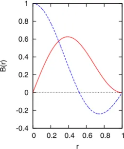
[image:4.595.53.547.532.706.2]

(5)

Figure 3. From Gourgouliatos et al. (2012) shows the toroidal magnetic field (red solid line) and the axial field (blue dashed line) as a function of the jet radius. Notice that the fields are zero at the jet boundary, resulting in jets that do not have a current sheet at the boundary.

4 S TA B I L I T Y O F C U R R E N T- S H E E T- F R E E J E T S

Once we have tested our numerical approach on the case with well-known analytical result, it makes perfect sense to consider a more complex flow which cannot be treated analytically. With this goal in mind, we opted to analyse the linear stability of current-sheet-free jets, whose equilibrium structure was recently studied by Gourgouliatos et al. (2012). These jets carry zero net poloidal cur-rent and the thermal gas pressure is an important dynamical com-ponent. This combination of thermal pressure and magnetic field enables us to avoid having surface currents at the jet boundary. The radial structure of the magnetic field is described by a rather complicated variant of the Grad–Shafranov equation, which in the general case can be solved only numerically. However, Gourgou-liatos et al. (2012) have identified two cases when the equation becomes tractable and found two families of analytical solutions. In our work, we analysed the linear stability of the solutions associ-ated with use of the poloidal magnetic flux function to describe the magnetic field. The magnetic field and gas pressure of this solution are given by equations (24)–(26) in Gourgouliatos et al. (2012). For our non-relativistic, the equations read

Bφ(r)=cαJ1(αr)−F r

α , (17)

Bz(r)=cαJ0(αr)−

2F

α2, (18)

P(r)=F

crJ1(αr)− F r

2

α2

+P0, (19)

whereP0is gas pressure on the axis. The free parameters are set to

bec=0.172,α=5.14 andF= −1.54 which puts the jet boundary atr=1. For the above choice of parameters, the maximum value of Bzis 1. In Fig.3we repeat the plots of the toroidal and axial magnetic fields from equations (17) and (18). These distributions can be combined with an arbitrary distributionvz(r) of the jet velocity, without upsetting the force balance. In this work we use a top hat velocity profile. The ambient pressure is constant and obtained by matching it to the pressure at the boundary of the jet. The plasma-β in the jet is, therefore, adjusted by varying the value ofP0.

Jets with current sheets have been studied before. The magnetic field configurations in equations (17) and (18) are certainly not

unique, but they are novel. The stability of jets with this magnetic field configuration has never been studied before. The absence of a current sheet may also be very desirable for numerical simulations where numerical resistivity can masquerade as a physical resistivity. For that reason, we study it here.

4.1 The base model

In order to prominently illustrate the effect of current-sheet-free magnetic field on the jet stability, we decided to use the unmagne-tized model withM=4 andη=0.1, whose stability we analysed in Section 3 (see Fig.2) as a reference, and to retain as much of its structure as possible. In particular, we retain the constant profile for the jet velocity in all magnetic models presented here.

It is very helpful to see the results of introducing the current-sheet-free magnetic field as a function of increasing magnetic field. Viewed as a progression, it becomes easier to pick out the trends. Consequently, Figs4,5and6show the stability analysis for both the pinch (m=0) and kink (m=1) modes whenβ=1, 1/2 and 1/4, respectively. Figs4–6are shown in the same format as in Fig.2. In all these three plots, we present the data for the fundamental mode and the first two reflection modes. Comparison of Figs2and

4shows reduced growth rates in the magnetic case withβ=1. The magnetic field is already dynamically important in theβ=1 jet. As we increase the magnetic field strength in Figs5and6, which correspond to strongly magnetized jets withβ=1/2 and 1/4, we see that the stability of the jet improves even further. The improve-ment in stability is particularly strong for the fundaimprove-mental modes. For the fundamental pinch mode, a wide window aroundkrj=1 appears, where this mode is not growing at all. A similar window of suppressed growth for the fundamental kink mode appears around krj=4. The results for the first two reflection modes also shows

improved stability properties of the magnetic model, but now in the

krj>>1 region, where we also observe complete suppression of

these modes. Fig.6(b) also shows evidence for some mode mix-ing between the fundamental mode and the second reflection kink mode at large wavenumbers, i.e. at short wavelengths. The mag-netic field used in Fig.6was strong enough to drastically alter the pressure profile of the jet, resulting in the mode mixing that we see in Fig.6(b).

Fig. 5has shown that for large regions of wavenumber space there are no unstable modes. Our method is based on a numerical search procedure. The interested reader may well ask: How we can be sure that there are absolutely no other unstable modes in the jet? Indeed, for a numerically motivated search process there is no ironclad way of showing that the dispersion relation has no further roots. However, it is possible to demonstrate that within a specified search space that is reasonably large, no further roots exist. (Recall the search strategy that was described in Fig.1.) Let us focus on ‘k rj=0.6’ in Fig.5(a). For that value of wavenumber,

we can plot out the amplitude of our dispersion relation in a two-dimensional domain given by (ω_r, ω_i)∈[0,1]×[0,0.3]. This is shown in the left-hand panel of Fig.7. We see clearly that there are no growing modes. Similarly, let us focus on ‘k rj=2.0’ in Fig.5(b).

For that value of wavenumber, we can plot out the amplitude of our dispersion relation in a two-dimensional domain given by (ωr, ωi)∈ [0,2]×[0,0.3]. This is shown in the right-hand panel of Fig.7. We can again see clearly that there is only one growing mode and that mode is the first reflection mode.

It is very interesting to ask whether the current-free aspect of the jet contributes significantly to jet stability. I.e. envision a scenario where the magnetic field configuration from equations (17) to (19)

[image:5.595.99.227.58.212.2]

(6)

[image:6.595.54.548.56.228.2] [image:6.595.53.547.283.456.2]

Figure 4. Corresponds to a magnetized current-sheet-free jet withM=4,η=0.1 andβ=1, i.e. the on-axis magnetic pressure is in equipartition with the gas pressure. Panel (a) shows the angular frequency (solid line) and temporal growth rate (dashed line) for them=0 mode while panel (b) shows the same for them=1 mode. The fundamental mode and first two reflection modes are shown.

Figure 5. Corresponds to a magnetized current-sheet-free jet withM=4,η=0.1 andβ=1/2, i.e. the on-axis magnetic pressure is twice the gas pressure. Panel (a) shows the angular frequency (solid line) and temporal growth rate (dashed line) for them=0 mode while panel (b) shows the same for them=1 mode. The fundamental mode and first two reflection modes are shown.

Figure 6. Corresponds to a magnetized current-sheet-free jet withM=4,η=0.1 andβ=1/4, i.e. the on-axis magnetic pressure is four times the gas pressure. Panel (a) shows the angular frequency (solid line) and temporal growth rate (dashed line) for them=0 mode while panel (b) shows the same for them=1 mode. The fundamental mode and first two reflection modes are shown.

[image:6.595.57.545.513.682.2]

(7)

[image:7.595.52.544.233.401.2]

Figure 7. Which is analogous to Fig.1, shows the search space that is used for finding fundamental and reflection modes in Fig.5. A range of values in (ωr, ωi) is selected and the amplitude of the complex dispersion relation is plotted for that range. The roots of the dispersion relation are easily identified as the

locations where the amplitude vanishes. Panel (a) corresponds to ‘k rj=0.6’ in Fig.5(a). By scanning the colours of the contours we see, therefore, that there is only one fundamental pinch mode. Panel (b) corresponds to ‘k rj=2.0’ in Fig.5(b). By scanning the colours of the contours we see, therefore, that there is one fundamental and one reflection kink mode.

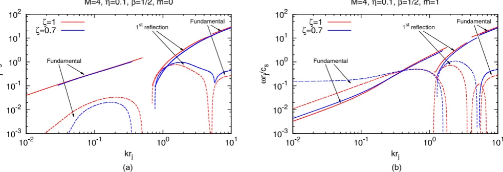
Figure 8. Intercompares two magnetized jets withM=4,η=0.1 andβ=1/2. Theξ=1.0 case, shown in red, is just the current-sheet-free jet that we have studied before in Fig.5. Theξ=0.7 case, shownin blue, has a current sheet at its boundary. Panel (a) shows the stability of them=0 mode. Panel (b) shows the stability of them=1 mode. Both figures show the fundamental and first reflection modes. For them=1 kink mode, the fundamental mode is much more stable for the current-sheet-free jet especially at longer wavelengths.

retained an overall helical form but the magnetic field were non-zero at the boundary of the jet. In that case, what are the changes in the jet stability? Realize, therefore, that equations (17)–(19) are structured so that the magnetic field goes to zero at the radius of the jet, i.e. atr=1. The magnetic field can be made to retain the same form but have non-zero magnetic field at the jet boundary if we replacer:=r/ξwithξ <1. In that case, the magnetic field will retain the same helical structure but it will have a non-zero value at the jet boundary. Fig.8intercompares two magnetized jets with M=4,η=0.1 andβ=1/2. Theξ =1.0 case, shown in red, is just the current-sheet-free jet that we have studied before in Fig.5

and is shown to provide a point of reference in Fig.8. Theξ=0.7 case, shown in blue, has a current sheet at its boundary. Fig.8(a) shows the stability of the fundamental and first reflectionm=0, i.e. pinch, modes. Fig.8(b) shows the stability of the fundamental and first reflectionm=1, i.e. kink, modes. For them=1 kink mode shown in Fig. 8(b), the fundamental mode is much more stable for the current-sheet-free jet, especially over a broad range of longer wavelengths. Note though that them=0 pinch mode in Fig.8(a) is slightly more stable for the jet with a current sheet. We ascribe that to the fact that the magnetic field is parametrized by

β, which is only evaluated at the jet’s axis. As a result, the radially averaged magnetic energy for theξ = 0.7 jet is larger than the radially averaged magnetic energy for theξ=1 jet. Consequently, them=0 mode in Fig.8(a) has slightly greater stability for the

ξ=0.7 jet than for theξ=1 jet. Them=1 mode is more susceptible to instabilities driven by current sheets. As a result, them=1 mode in Fig.8(b) has substantially greater stability at long wavelengths for theξ=1 jet than theξ=0.7 jet. In all cases, we find that the first reflection mode for theξ=1 jet has improved stability compared to theξ=0.7 jet.

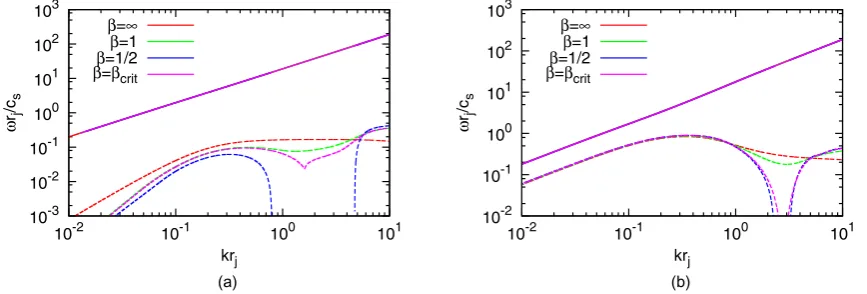
Figs9and10illustrate how the stability properties of the mag-netic model vary with the magmag-netic field strength. Fig.9shows the evolution of the fundamental pinch and kink modes. One can see that the results for low- and high-magnetization models are qualitatively different – whereas the dispersion curves for the low-magnetization models appear as slightly deformed versions of the non-magnetic model, the high-magnetization models show splitting of the curves into two branches separated by finite-size windows of suppressed growth. The bifurcation occurs aroundβ=1. Outside of the win-dows, the growth rates show only minor changes withβ. Fig.10

shows the evolution of the first reflected pinch and kink modes. The results are reminiscent of those for the fundamental modes. Regions of suppressed growth appear in thekrj>1 zone (they may or may

not continue to infinity). Outside of these windows the growth rates remain more or less unchanged.

In general, the observed instabilities can be driven either by the velocity gradient, i.e. Kelvin–Helmholtz (KH) instability, gas pres-sure fluctuations or the magnetic forces, i.e. current-driven (CD) instability. Forβ= ∞the jet is unmagnetized, so that we can be

(8)

[image:8.595.89.508.58.205.2]

Figure 9. We show the fundamental modes for theM=4,η=0.1 jets withβ=infinity,β=1,β=βcritandβ=1/2. I.e. the different colours show the enhancement of jet stability as the magnetic field is increased. In all cases the current-sheet-free magnetic configuration was used. Panel (a) shows them=0 fundamental mode while panel (b) shows them=1 fundamental mode.βcritis theβvalues when the separation of modes starts to occur and their values are 0.95 (m=0) and 0.76 (m=1) The real parts of the angular frequency, when they are plotted, overlie each other in both the figures.

Figure 10. We show the first reflection modes for theM=4,η=0.1 jets withβ=infinity,β=1 andβ=1/ 2. I.e. the different colours show the enhancement of jet stability in the reflection modes as the magnetic field is increased. In all cases the current-sheet-free magnetic configuration was used. Panel (a) shows them=0 first reflection mode while panel (b) shows them=1 first reflection mode.

sure that we are dealing exclusively with the KH instability. An increase of the growth rate for lower values ofβwould be indica-tive of a CD instability. Figs9and10 show a small increase of the growth rate only atkrj∼10. Thus, one may conclude that the

imposed current-sheet-free magnetic field partially suppresses the KH instability and does not introduce strong CD instabilities. To understand CD instabilities it is important to find the resonant sur-face where the resonance condition (k B=k B_z0+(m/r)Bz0=0)

holds. When this surface resides inside the jet, the jet becomes un-stable to CD instability. Realize, therefore, that the CD instability becomes very prominent when the magnetic field in the jet has a constant pitch angle, as is the case in the model of Bodo et al. (2013). In our model, the magnetic field in the jet has a range of pitch angles, see Fig.3. Consequently, our model always has a resonant surface inside the jet regardless ofkandmvalue. (The resonant surface exists even for the extremely short wavelength orm= −1 case.) Accordingly, both KH and CD instabilities appear in all our results. Bodo et al. (2013) have a magnetic field with a constant pitch angle. Consequently, the CD instability of their model is limited to a cer-tain wavenumber (k0∼1/P, wherePis the pitch of the magnetic

field). They show distinct CD instability in their figs 4–8 for highly magnetized jets. However, our model does not show dramatic dif-ference when the CD instability becomes dominant since our model does not have a limiting wavenumber. Furthermore, please realize

that the jets used in the study by Bodo et al. (2013) have zero pres-sure, which exaggerates the role of the CD instability. The jets used in our study have a finite pressure which permits sound waves to carry away fluctuations. The presence of a finite sound speed, which is comparable to the Alfven speed, greatly suppresses the role of the CD instability.

The bifurcation of dispersion curves is a particularly interesting property of our magnetic models. In order to further localize this bifurcation, we need to study the dependence onβin greater de-tail. To this aim we adopted the following procedure. We pick a wavenumber in Fig.2and start with the real and imaginary angu-lar frequencies of the unmagnetized jet. For that wavenumber, we progressively increase the magnetic field and re-evaluate the real and imaginary angular frequencies. This is done for increasing val-ues of the magnetic field till the imaginary part of the frequency becomes negligibly small. Since the fundamental modes are well separated from the first reflection modes, it is reasonable to assume that once we start with a fundamental mode, the modes that we find via this process continue to be the fundamental modes. We repeat this process for all wavenumbers that range from 0.01 to 10. As the result, we obtain the growth rateωIrj/csas a function of two

variables –krjand 1/β. Fig.11shows the results for them=0 and 1

fundamental modes. The green line in these plots shows the location where the growth rate drops below 10−3_{. Interestingly, for the pinch}

[image:8.595.85.516.272.419.2]

(9)

[image:9.595.47.546.59.217.2] [image:9.595.51.545.282.438.2]

Figure 11. The imaginary part of the fundamental modes is colour coded. Consequently, panel (a) shows the colour coded value of the imaginary part of the angular frequency, i.e.ωIrj/csas a function of wavenumber and increasing magnetic field (denoted by 1/β) for them=0 fundamental mode. Panel (b) shows the same information for them=1 fundamental mode. The green lines in panels (a) and (b) identify the boundary of the regions past whichωIrj/csdrops below a value of 10−3_.

Figure 12. The same exercise as in Fig.11can now be repeated for the first reflection mode. Panel (a) is analogous to Fig.11(a) with the exception that it shows the colour coded imaginary part of the angular frequency for them=0 first reflection mode. Similarly, panel (b) is analogous to Fig.11(b) and shows the colour coded imaginary part of the angular frequency for them=1 first reflection mode. The green lines in panels (a) and (b) identify the boundary of the regions past whichωIrj/csdrops below a value of 10−3.

mode the bifurcation occurs almost simultaneously at two separate wavenumbers. Their corresponding windows of suppressed growth rapidly merge and form a wide single window. In contrast, for the kink mode the bifurcation occurs in a single point and the window of instability suppression remains relatively narrow.

Fig.12shows the results for the first reflection pinch and kink modes. Unfortunately, these plots are less informative on the onset of the bifurcation – it is not clear whether it occurs at large but finite wavenumber or at infinity. However, one may still conclude that atβ=1 the short-wavelength reflection modes become stabilized over a wide spectral range.

4.2 Other models

In the previous section we studied jets with fixed parametersM=4,

η=0.1. In part, this was dictated by the fact that one of the models studied in the seminal paper by Cohn (1983) had exactly these pa-rameters and we could use this model as a reference point. However, AGN jets can be much lighter than the ambient gas that they propa-gate through, whereas protostellar jets can be even heavier than the ambient gas that they propagate through. Furthermore, the Mach

numbers of both types of jets can be quite large. For that reason, the next two subsections explore the stability properties of jets with much larger Mach numbers than our canonical jet and with a range of density ratios.

4.2.1 Very light jet

In this section, we consider a current-sheet-free jet withM=10,

η=0.01. These parameters are closer to those of AGN jets com-pared to the base model. We repeated all the steps that we undertook in Section 4.1 except that in this section we consider the current-sheet-free jet withM=10,η=0.01. The results in this section are presented in the same format as the previous section. Figs13–16

are to be compared with Figs9–12of the Section 4.2, respectively. Inspection of the data shows that the two major trends found for the base model are repeated for the very light jet: (1) the growth rates of unstable modes are normally reduced with increased magneti-zation. (At some wavenumbers the growth rate of reflection modes may actually increase but only weakly.) and (2) when the magnetic field becomes dynamically important, i.e. at aroundβ=1, windows of fully suppressed instability appear.

(10)

[image:10.595.87.511.56.205.2]

Figure 13. We study a current-sheet-free jet withM=10,η=0.01 and a range of plasma-βs. The results of stability analysis for the fundamentalm=0 and

[image:10.595.85.516.265.412.2]

m=1 modes are shown in panels (a) and (b). Increasing the strength of the current-sheet-free magnetic field dramatically improves the stability properties of light jets. Compare this figure to Fig.9.

Figure 14. We study a current-sheet-free jet withM=10,η=0.01 and a range of plasma-βs. The results of stability analysis for the first reflectionm=0 andm=1 modes are shown in panels (a) and (b). Increasing the strength of the current-sheet-free magnetic field dramatically improves the stability properties of light jets. Compare this figure to Fig.10.

Figure 15. The imaginary part of the fundamental modes is colour coded. Consequently, panel (a) shows the colour coded value of the imaginary part of the angular frequency, i.e.ωIrj/csas a function of wavenumber and increasing magnetic field (denoted by 1/β) for them=0 fundamental mode. Panel (b) shows the same information for them=1 fundamental mode. The green lines in panels (a) and (b) identify the boundary of the regions past whichωIrj/csdrops below a value of 10−3.

The most significant quantitative differences with the base model are observed in the data for fundamental modes. One can see that already in the non-magnetic case, the growth rates are systematically lower. For magnetic models, the windows of suppressed instability

are substantially broader – forβ=0.5 the instability is suppressed at a range of 0.05 1< krj<8.4 (m=0), 0.40< krj<9.1 (m=1).

For reflection modes, the growth rates are less affected. The domain of their instability is shifted towards lower wavenumbers.

[image:10.595.59.547.472.628.2]

(11)

[image:11.595.53.541.60.215.2]

Figure 16. Panel (a) is analogous to Fig.15(a) with the exception that it shows the colour coded imaginary part of the angular frequency for them=0 first reflection mode. Similarly, panel (b) is analogous to Fig.15(b) and shows the colour coded imaginary part of the angular frequency for them=1 first reflection mode. The green lines in panels (a) and (b) identify the boundary of the regions past whichωIrj/csdrops below a value of 10−3.

Figure 17. The results of stability analysis of a current-sheet-free jet withM=20,η=10 and a range of plasma-βs for the fundamentalm=0 andm=1 modes are shown in panels (a) and (b). By comparing this figure to Figs9and13we see that the stability of the heavy jet is not improved as much as the stability of the light jets when the current-sheet-free magnetic field is increased.

The bulk of this shift is already present in the non-magnetic case and hence can be attributed to the properties of KH instability.

4.2.2 Heavy jet

In our last example we consider heavy jet withM=20,η=10. Just as we did for the very light jet, we repeated all the steps of base model study and presented the results in the same format (see Figs17–20). Inspection of these plots shows the same trends again. The magnetic field keeps playing the same role as before in reducing the growth rate of unstable modes and creating windows of suppressed instability. The bifurcations occur atβ ∼1 again. In contrast to the very light jets, these windows are now somewhat narrower than in the base model. However, the domain of instability for first reflection modes is still shifted towards lower wavenumbers.

5 D I S C U S S I O N

Stability is undoubtedly one of the key issues in the physics of cosmic jets, which has many sides to it. Instabilities are likely to lead to dissipation of both the bulk kinetic and magnetic energies. The dissipated energy can then be emitted via different thermal and non-thermal mechanism and hence the stability issue is tightly con-nected to the problem of observed emission. Instabilities can result

in jets developing large- and small-scale structures like wiggles, he-lical patterns, knots, etc. and thus relates to the issue of the observed jet morphology. But probably the most important of all is the issue of jet survival. As we have already discussed in the Introduction, in contrast to their terrestrial and laboratory counterparts, the astro-physical jets exhibit remarkable ability to preserve their integrity over huge distances – distances that can exceed the initial jet radius by up to a billion times! In extragalactic radio sources of type 2 in the Fanaroff–Riley classification, AGN jets can be traced all the way up to the leading hotspots, which are hundreds of kiloparsecs away from galactic nuclei. In the type 1 sources, the AGN jets are shorter and are seen to turn into what appears to be slow turbulent plumes. This transition is reminiscent of what happens to terrestrial supersonic jets due to KH instability.

Linearization of governing equations is the traditional way of studying stability of dynamical systems. The problem is then re-duced to the eigenvalue problem for linear equations, which are sig-nificantly simpler compared to the original non-linear ones. This is a very powerful mathematical tool, particularly when the eigenfunc-tions can be expressed in terms of well-known analytic funceigenfunc-tions. Unfortunately, this is not always the case and to achieve solutions to the linearized system one is often forced to consider rather over-simplified equilibrium configurations. In more general setting, the eigenvalue problem has to be solved numerically. This is the way

[image:11.595.80.514.275.422.2]

(12)

[image:12.595.87.512.57.205.2] [image:12.595.50.545.245.403.2]

Figure 18. The results of stability analysis of a current-sheet-free jet withM=20,η=10 and a range of plasma-βs for the first reflectionm=0 andm=1 modes are shown in panels (a) and (b).

Figure 19. The imaginary part of the fundamental modes is colour coded. Consequently, panel (a) shows the colour coded value of the imaginary part of the angular frequency, i.e.ωIrj/csas a function of wavenumber and increasing magnetic field (denoted by 1/β) for them=0 fundamental mode. Panel (b) shows the same information for them=1 fundamental mode. The green lines in panels (a) and (b) identify the boundary of the regions past whichωIrj/csdrops below a value of 10−3_.

Figure 20. The same exercise can now be repeated for the first reflection mode. Panel (a) is analogous to Fig.19(a) with the exception that it shows the colour coded imaginary part of the angular frequency for them=0 first reflection mode. Similarly, panel (b) is analogous to Fig.19(b) and shows the colour coded imaginary part of the angular frequency for them=1 first reflection mode. The green lines in panels (a) and (b) identify the boundary of the regions past whichωIrj/csdrops below a value of 10−3.

the linear stability analysis of astrophysical jets is currently evolv-ing. Following Bodo et al. (2013), and also significantly amplifying on that work, we have applied this approach to cylindrical magne-tized jets free of surface currents (Gourgouliatos et al.2012) and demonstrated its robustness and efficiency. We have found that such

magnetic field inhibits growth of KH instability modes and does not introduce strong CD instabilities. When the magnetic field exceeds the equipartition strength, the instabilities become fully suppressed for a whole range of wavelengths. This is particularly significant for the so-called fundamental modes, which in some of our cases

[image:12.595.56.546.463.618.2]

(13)

become suppressed for wavelengths ranging from a fraction to a hundred of jet radii. However, not all modes are suppressed and strictly speaking the jets remain linearly unstable.

The accepted wisdom says that unstable equilibrium solutions cannot describe natural phenomena – they are self-destructing. However, they can still be relevant as approximations of reality. For example, perturbations, which grow rapidly while their ampli-tude is small, may saturate in the non-linear regime (e.g. O’Neill, Beckwith & Begelman 2012). Moreover, unstable solutions may remain near the equilibrium for some time even if eventually they move far away from it. Only numerical solution of original non-linear equations can answer these questions. This is why numerical simulations have become a popular tool for stability studies (see Mizuno et al.2012; O’Neill et al.2012; Porth & Komissarov2014

for some of the recent examples). This is one of the ways our study of current-sheet-free jets will have to be continued eventually.

As far as the linear analysis is concerned, one of the main lim-itations of the present study is the neglect of the velocity shear within the jet. We expect that a sheared jet will show even better stability properties, as shear tends to destroy coherence of perturba-tions and suppresses small-scale instabilities (Chandrasekhar1961; Michalke1964; Blumen, Drazin & Billings1975). The study of shear in the jet is deferred to a subsequent paper. This study also needs to be extended to the relativistic regime, and we defer that also to a subsequent paper.

In this paper we have addressed the long-term linear stability of magnetized jets propagating through a constant density medium. We expect that these calculations are applicable to the largest scales of astrophysical jets from AGN, i.e. on the scales of tens to hundreds of kiloparsec, like those in the famous radio galaxy Pictor A. We have studied the stability of such a possible cylindrical magnetized jet configuration.

As they propagate through realistic environments, cosmic jets are not quite cylindrical but exhibit a certain amount of lateral expan-sion. In the superfast magnetosonic regime, the speed of steady-state non-relativistic jets remains almost constant and due to the magnetic flux conservation the azimuthal component of magnetic field decreases as 1/rj, where poloidal component as 1/rj2, which

is much faster. Since the radius of astrophysical jets increases by many orders of magnitude, especially at the base of the jet where it is launched, it is inconceivable that the poloidal component is the same order as the azimuthal one everywhere along the jet. For magnetically accelerated jets, the azimuthal component becomes of the order as the poloidal one at the Alfven surface, which is only a little bit closer to the origin than the fast-magnetosonic surface. The dominance of the toroidal magnetic field will trigger CD insta-bilities with the jet, like sausage and the kink modes. As a result, some toroidal magnetic field will be destroyed. We hypothesize that after entering a nearly constant density profile in the intergalactic medium a narrow AGN jet finds a cylindrical equilibrium configu-ration with similar toroidal and poloidal magnetic fluxes. This pro-vides a natural scenario where extragalactic jets could naturally re-lax towards the magnetic field configurations that we have explored here.

For relativistic jets, the transition from jet launching to free prop-agation can be even more interesting. In this regime one has to distinguish between the magnetic field as measured in the source frame and in the jet frame. For the jet magnetostatic equilibrium it is the jet frame magnetic field which matters. While the poloidal component of this field still varies as 1/r2

j, the azimuthal one varies

as 1/rjγj

, whereγjis the jet Lorentz factor as measured in the

source frame. Studies of relativistic magnetized jets show that they

continue to accelerate in the superfast-magnetosonic regime – their Lorentz factor increases (Komissarov et al.2009). When such jets are confined by an external gas with total pressurePtot∼z−κ, where

zis the distance along the jet and 0< κ <2, the Lorentz factor grows as∼rj(Komissarov et al.2009) and thus the azimuthal

mag-netic field decreases at the same rate as the poloidal one. Because of this effect, an equilibrium configuration with comparable poloidal and azimuthal components of magnetic field can be maintained for longer.

One additional interesting possibility for enhancing the stabil-ity of extragalactic jets is that the lateral expansion of astrophysical jets helps to stabilize them. Indeed, such an expansion constantly in-creases the communication time across the jet and thus slows down the development of instabilities. Whenκ >2 the causal communi-cation across the jets is completely lost and the jets should become absolutely stable to global instabilities. Recent numerical simula-tions provide very nice support for this idea (Porth & Komissarov

2014).

6 C O N C L U S I O N S

Normally, linear stability analysis of astrophysical jets is based on simplifying assumptions about the jet’s velocity profile and mag-netic field structure – the jet’s velocity is usually taken to be a top-hat velocity profile and its magnetic field either constant in the longitudinal direction or restricted to loops of magnetic field. The simplifications are needed in to obtain closed-form analytical rep-resentation for the perturbed variables in the jet. These analytical functions usually take the form of modified Bessel functions or hypergeometric functions. In this paper we adopt a different, nu-merically motivated approach to linear stability. With this approach, the jet is allowed to have any velocity profile and any unperturbed magnetic field structure.

Specifically, we focus on magnetic field structures that are free of current sheets on the surface of the jet (Gourgouliatos et al.2012). We believe that these magnetic field structures are more realistic and confer some better stability properties to the jet. The non-relativistic MHD equations are linearized around a general velocity profile in the jet and a general magnetic field in the jet. The resulting linear equations are solved numerically inside the jet. At the radial boundary of the jet, we follow convention and match the pressure and displacement from inside the jet to the corresponding analytical solution in the ambient medium.

We find that current-sheet-free magnetic field can significantly reduce the jet instability compared to the non-magnetic case. For weak magnetic fields (defined in terms of plasma-β, i.e. the ratio of gas to magnetic pressure) the jets display the well-known fun-damental and reflection modes for the pinch and kink instabilities. However, as the magnetic field is increased slightly past equipar-tition, the stability properties of these modes improve. The most dramatic improvement, both for pinch and kink instabilities, occurs in the fundamental modes, particularly at long wavelengths. These are the wavelengths that are known to become most pernicious to jet stability when the evolution enters the non-linear regime. The reflection modes, both for the pinch and kink instability, also be-come progressively more stable with decreasing plasma-β, but to a lesser degree.

AC K N OW L E D G E M E N T S

DSB acknowledges support via NSF grants NSF-AST-1009091, NSF-ACI-1307369 and NSF-DMS-1361197. DSB and ML also

(14)

acknowledge support via NASA grants from the Fermi program as well as NASA-NNX 12A088G. Several simulations were per-formed on a cluster at UND that is run by the Center for Research Computing. Computer support on NSF’s XSEDE and Blue Waters computing resources is also acknowledged.

R E F E R E N C E S

Begelman M. C., 1998, ApJ, 493, 291

Blandford R. D., Payne D. G., 1982, MNRAS, 199, 883 Blandford R. D., Znajek R. L., 1977, MNRAS, 179, 433

Blumen W., Drazin P. G., Billings D. F., 1975, J. Fluid Mech., 71, 305 Bodo G., Mamatsashvili G., Rossi P., Mignone A., 2013, MNRAS, 434,

3030

Chandrasekhar S., 1961, Hydrodynamic and hydromagnetic stability, Inter-national Series of Monographs on Physics, Oxford, Clarendon Cohn H., 1983, ApJ, 269, 500

Cox J. P., 1980, Theory of Stellar Pulsation. Princeton Univ. Press, Princeton, NJ

Gourgouliatos K. N., Fendt C., Clausen-Brown E., Lyutikov M., 2012, MNRAS, 419, 3048

Hardee P. E., 1979, ApJ, 234, 47

Hardee P. E., 1982, ApJ, 257, 509

Istomin Y. N., Pariev V. I., 1996, MNRAS, 281, 1

Kim J., Kim H. I., Choptuik M. W., Lee H. M., 2012, MNRAS, 424, 830 Komissarov S. S., Barkov M. V., 2009, MNRAS, 397, 1153

Komissarov S. S., McKinney J. C., 2007, MNRAS, 377, L49

Komissarov S. S., Vlahakis N., Koenigl A., Barkov M. V., 2009, MNRAS, 394, 1182

Lovelace R. V. E., 1976, Nature, 262, 649 Lyubarskii Y. E., 1999, MNRAS, 308, 1006

McKinney J. C., Blandford R. D., 2009, MNRAS, 394, L126 McKinney J. C., Narayan R., 2007, MNRAS, 375, 513 Michalke A., 1964, J. Fluid Mech., 19, 543

Mizuno Y., Lyubarsky Y., Nishikawa K. I., Hardee P. E., 2012, ApJ, 757, 16

Narayan R., Li J., Tchekhovskoy A., 2009, ApJ, 697, 1681

O’Neill S. M., Beckwith K., Begelman M. C., 2012, MNRAS, 422, 1436 Payne D. G., Cohn H., 1985, ApJ, 291, 655

Porth O., Komissarov S. S., 2014, preprint (arXiv:1408.3318) Ray T., 2012, EAS Publ. Ser., 58, 105

Rees M. J., 1978, Nature, 275, 516

Reipurth B., Bally J., Fesen R. A., Devine D., 1998, Nature, 396, 343 Tomimatsu A., Matsuoka T., Takahashi M., 2001, Phys. Rev. D, 64,

123003

A P P E N D I X A : C O M P O N E N T S O F T H E M AT R I X AA N D B

All the components of the matrix Aand column vector B for solving seven algebraic equations (AX=M), equation 12) described in Section 3 are given by

A= ⎡ ⎢ ⎢ ⎢ ⎢ ⎢ ⎢ ⎢ ⎢ ⎢ ⎢ ⎢ ⎢ ⎢ ⎢ ⎣

0 −im_r iρ0 0 − dB_φ0

dr +

Bφ0 r

ikB_z0 −im_rBz0

0 −ik 0 iρ0 −

dBz0

dr −ikBφ0 im_rBφ0

0 0 0 0 0 0

−iBφ0

ρ0 0 ikB 0 0 i 0

−ikB_ρ0 0 −im_r kB −ikkB 1_r+ k dvz0

dr −i

m

r −ik

−γ P0 ρ0 0 0 0 0 0

0 −1 0 0 0 −Bφ0 −Bz0

⎤ ⎥ ⎥ ⎥ ⎥ ⎥ ⎥ ⎥ ⎥ ⎥ ⎥ ⎥ ⎥ ⎥ ⎥ ⎦ , B= ⎡ ⎢ ⎢ ⎢ ⎢ ⎢ ⎢ ⎢ ⎢ ⎢ ⎢ ⎢ ⎢ ⎢ ⎣ 0

−ρ0 dvz0

dr δvr

−kBδvr Bφ0

ρ0 ddρ0r +Brφ0 −

dBφ0

dr

δvr kB

kBC − rkBD −ρ01ddρ0r

δvr 0 −δ ⎤ ⎥ ⎥ ⎥ ⎥ ⎥ ⎥ ⎥ ⎥ ⎥ ⎥ ⎥ ⎥ ⎥ ⎦

, X=

⎡ ⎢ ⎢ ⎢ ⎢ ⎢ ⎢ ⎢ ⎢ ⎢ ⎢ ⎢ ⎢ ⎢ ⎣ δρ δP δvφ δvz δBr δBφ δBz ⎤ ⎥ ⎥ ⎥ ⎥ ⎥ ⎥ ⎥ ⎥ ⎥ ⎥ ⎥ ⎥ ⎥ ⎦ , (A1)

whereC= m_r dBφ0

dr +k

dBz0

dr andD=kBz0+2_rmBφ0. Note that all components does not contain derivatives of perturbation variables andδvr

andδonly appear inB

A P P E N D I X B : A S Y M P T OT I C B E H AV I O U R O F S O L U T I O N S AT S M A L L R A D I I

(i)m=0

The power laws of all the perturbation variables deduced from linearized equation by the assumption ofδρ∼rαnearr=0 are provided as

δρ=δρ∗_rα_; _δP ₌_δP∗_rα_; _δv

r=δvr∗rα+1; δvφ=δvφ∗rα+1; δvz=δvz∗rα;

δBr=δBr∗rα+1; δBφ=δB∗φrα+1; δBz=δBz∗rα.

Up to leading order (after cancelling out leading order ofr) equations (4)–(11) become

iδρ

∗ ρ0

+(α+2)δv∗_r−ikδv∗_z =0, (B1)

(15)

α(B_z0δB_z∗+δP∗)=0, (B2)

iρ0δv∗_φ=2B_φ0δBr∗−ikBz0δB_φ∗, (B3)

iρ0δv∗_z=ikδP∗, (B4)

δB∗

r = −kBδv∗_r, (B5)

i δB_φ= −(α+2)B_φ₀δv_r∗−ikB_z0δv_φ∗+ikB_φ0δv∗z, (B6)

(α+2)δB_r∗=ikδB_z∗, (B7)

δP∗

P0

=γδρ_ρ∗

0

. (B8)

SinceδB_z∗andδP∗are expressed in terms ofδv_r∗,αmust be 0 for the non-trivial solution ofδv∗_r. By substitutingδρ∗andδv_z∗in equation (1) forδP∗using equations (B4) and (B8), we can obtain an expression ofδP∗in terms ofδv_r∗, i.e.

δP∗₌ 2iδv∗r

γ P0− k

2 ρ0

. (B9)

In addition, equations (B5) and (B7) give

δB∗

z = 2iB_z0

δv∗r. (B10)

Since the definition of total pressure perturbation is δ∗=δP∗+Bφ0δB_φ∗r2+Bz0δB_z∗, we can obtainδ∗(r=0)=Bz0δB_z∗+δP∗in

terms ofδv_r∗by making substitutions of equations (B9) and (B10). (ii)|m| ≥1

Likem=0, the perturbed variables have following relations nearr=0:

δρ=δρ∗_rα_; _δP₌_δP∗_rα_; _δv_r₌_δv∗

rrα−1; δvφ =δv∗φrα−1; δvz=δvz∗rα;

δBr=δBr∗rα−1; δBφ=δBφ∗rα−1; δBz=δBz∗rα.

After substitution of above relation in equations (4)–(11) provides

αδv∗

r −imδvφ∗=0, (B11)

iρ0δv∗_r= −ikB∗δBr∗−αδ∗−2Bφ0δB∗φ, (B12)

iρ0δv∗_φ=2B_φ0δBr∗−ikBz0δB_φ∗+im(Bz0δB_z∗+δP∗), (B13)

iρ0δv∗_z+ρ0v_z0δv∗r =Bz0δBr∗+i (k−m)Bφ0δBφ∗+ikδP∗, (B14)

δB∗

r = −kB∗δv∗r, (B15)

i δB∗_φ= −αB_φ₀δv_r∗−ikB_z0δv_φ∗, (B16)

αδB∗

r −imδBφ∗=0, (B17)

δP∗

P0

=γδρ_ρ∗

0

, (B18)

wherek_B∗=mB_φ₀+kB_z0andδ∗=δP∗+B_φ0δBφ∗+Bz0δB_z∗. Equations (B11) and (B15)–(B17) give the expressions ofδv_φ∗,δB_r∗and

δB∗

φin terms ofδv∗r. Furthermore, making substitutions ofδBr∗andδBφ∗inδ∗definition also givesδ∗dependent only onδv∗r. We make a further substitution of last term of angular momentum equation (equation B13) toδ∗−B_φ₀δB_φ∗and finally obtain an expression in terms ofδv∗_r: