An Empirical Demonstration of the Probabilistic Upper Bound of the Adaptive Boosting Test Error

(1)

Rochester Institute of Technology

RIT Scholar Works

Theses Thesis/Dissertation Collections

8-11-2016

An Empirical Demonstration of the Probabilistic

Upper Bound of the Adaptive Boosting Test Error

Paige Houston

[email protected]

Follow this and additional works at:http://scholarworks.rit.edu/theses

This Thesis is brought to you for free and open access by the Thesis/Dissertation Collections at RIT Scholar Works. It has been accepted for inclusion in Theses by an authorized administrator of RIT Scholar Works. For more information, please [email protected].

Recommended Citation

(2)

R

OCHESTER

I

NSTITUTE OF

T

ECHNOLOGY

M

ASTERS

T

HESIS

An Empirical Demonstration of

the Probabilistic Upper Bound of

the Adaptive Boosting Test Error

Author:

Paige H

OUSTON

Supervisor:

Dr. Ernest F

OKOUÉ

A Thesis Submitted in Partial Fulfillment of the Requirements

for the Degree of Master of Science in Applied Statistics

in the

School of Mathematical Sciences

College of Science

(3)

i

Declaration of Authorship

I, Paige HOUSTON, declare that this thesis titled, “An Empirical

Demonstra-tion of the Probabilistic Upper Bound of the Adaptive Boosting Test Error” and the work presented in it are my own. I confirm that:

• This work was done wholly or mainly while in candidature for a re-search degree at this University.

• Where any part of this thesis has previously been submitted for a de-gree or any other qualification at this University or any other institu-tion, this has been clearly stated.

• Where I have consulted the published work of others, this is always clearly attributed.

• Where I have quoted from the work of others, the source is always given. With the exception of such quotations, this thesis is entirely my own work.

• I have acknowledged all main sources of help.

• Where the thesis is based on work done by myself jointly with others, I have made clear exactly what was done by others and what I have contributed myself.

Signed:

(4)

ii

Committee Approval Form

Ernest Fokoué, Thesis Advisor,

Associate Professor, School of Mathematical Sciences Date

Steven LaLonde, Committee Member,

Associate Professor, School of Mathematical Sciences Date

Mei Nagappan, Committee Member,

Assistant Professor, Golisano College of Computing

and Information Sciences Date

Daniel Lawrence, Honorary Committee Member,

(5)

iii

ROCHESTER INSTITUTE OF TECHNOLOGY

Abstract

Ernest Fokoué

School of Mathematical Sciences

Master of Science in Applied Statistics

An Empirical Demonstration of the Probabilistic Upper Bound of the Adaptive Boosting Test Error

by Paige HOUSTON

(6)

iv

List of Figures

1.1 Training Error from Both Boosting Functions . . . 8

2.1 Training and Test Error on Large n Small p Datasets . . . 18 2.2 Training and Test Error on Large p Small n Datasets . . . 19

3.1 Training and Test Error on Imbalanced Datasets of Size 250 X 17 . . . 26 3.2 Training and Test Error on Imbalanced Datasets of Size 80 X 17 27 3.3 Training and Test Error on Imbalanced Datasets of Size 250 X

1200 . . . 27 3.4 Training and Test Error on Imbalanced Datasets of Size 80 X

1200 . . . 28 3.5 Training and Test Error on Balanced Datasets of Size 250 X 17 29 3.6 Training and Test Error on Balanced Datasets of Size 80 X 17 . 30 3.7 Training and Test Error on Balanced Datasets of Size 250 X 1200 30 3.8 Training and Test Error on Balanced Datasets of Size 80 X 1200 31

(9)

Chapter 1

Introduction

Statistical Machine Learning is used to construct a model or relationship between a set of parameters, or predictor variables, and a response to be able to predict results. First we must define a function space,F, where our model lives. We never know the actual model, or relationship, between the predictors and the response, so it is crucial to define a function space. It is impossible to consider every function when looking for the "best" model, so by defining a function space, we can narrow down our search for the best model to just linear classifiers, polynomial classifiers, or kernels, etc. (Fokoue, 2015a).

The way we determine what is the "best" model is by analyzing the risk function. We essentially have two risk functions, the Theoretical Risk, or our Generalization Error, denoted byR(f), and the Empirical Risk, or Training Error denoted by Rˆn(f) where f is a function in our function space F, or

f ∈F (Fokoue, 2015a). The two functions are defined by the following:

R(f) =E[l(Y, f(X))]

ˆ

Rn(f) = 1

n

X

i=1

[l(Yi, f(Xi))],

(10)

Chapter 1. Introduction

The best possible function to model our data is denoted byf∗, and it is the one that minimizes the risk:

f∗ = argmin f

{R(f)}.

In practice,f∗ cannot be found, so we estimate it usingfˆn. Since we cannot

simply choose a function with no background information that will

happen to be close to our best functionf∗, we, instead, look at all functions

f ∈F, and choose the one that yields an empirical risk,Rˆn(f), closest to our theoretical risk,R(f). However, we never know what the true error is in practice, so Vapnik and Chervonenkis derived an upper bound on the theoretical risk. This way we can know, generally, how large the error will be, instead of having no information on it at all. This theorem immediately follows in Section 1.1 (Fokoue, 2015a).

1.1

Vapnik and Chervonenkis Bound

Vapnik and Chervonenkis (1971) derived a bound for the theoretical risk. Their theorem is the following, as quoted directly from Fokoue, 2015a:

Theorem 1(Vapnik and Chervonenkis Bound). LetF be a class of functions

implementing [some] learning machines, and let ζ = V Cdim(F) be the VC

di-mension ofF. Let the theoretical and empirical risk be defined as earlier and con-sider any data distribution in the population of interest. ∀f ∈ F, the prediction error (theoretical risk) is bounded by

R(f)₆Rˆn(f) +

s

ζ(log2n

ζ + 1)−log

η

4

n ,

with probability of at least1−η. or

P r (

TestError₆TrainError+

s

ζ(log2_ζn + 1)−logη₄

n

)

>1−η

(11)

A question we can ask is the following: Is there a more general takeaway from this theorem? Can we generate a probabilistic bound for the theoretical error in the form of the following equation:

R(f)₆Rˆn(f) +φ(. . .)

The above equation suggests that our theoretical risk can be bounded by a shift of the empirical risk by φ(. . .) which is simply a function based on unknown parameters at this time.

Now we will revisit which function space,F to choosef from. As pre-viously mentioned,F can be any of, but not limited to, the following:

• Linear Classifiers

• Kernel

• Ensembles

– Bagging

– Random Forest

– Boosting

This list is just to give an idea of how many options there are, and this is not even a small fraction of all function spaces. However, in this thesis, we will focus on the Adaptive Boosting Algorithm, and how its generalized error can be bounded.

1.2

Adaptive Boosting

The Adaptive Boosting Algorithm is a classification method used in ma-chine learning (Abney, Schapire, and Singer, 1999). The defined algorithm can be seen in Algorithm 1.

(12)

Algorithm 1The Adaptive Boosting Algorithm

1: Let the following be defined as stated:

2: Training data: Dn ={(xi, yi) :xi ∈X, yi ∈ {−1,+1}, i= 1,2, . . . , n}.

3: Weak learners:ht(x)fort = 1,2, . . . , T :X → {−1,+1}.

4: Error associated with the weak learners: tfort= 1,2, . . . , n.

5: Initialized weights:D1(i) = _n1 fori= 1,2, . . . , n.

6: Choosehtsuch that the error is minimized.

7: Chooseαt= 1₂log1−_tt.

8: Update fori= 1,2, . . . , n,

Dt+1 =

Dt(i)

Zt

∗

eαt_, _if_h

t(xi)6=yi

e−αt_, _if_h

t(xi) = yi

,

meaning that

Dt+1=

Dt(i) exp −αtyiht(xi)

Zt

,

whereZtis a normalization factor chosen so thatDt+1 is a distribution.

9: The final output is

H(x) = sign

T

X

t=1

αtht(x)

(13)

at least one datum can be classified in more than one group (Schapire and Singer, 2000; Schapire and Singer, 1999; Abney, Schapire, and Singer, 1999). However, we will be using single-label datasets with a binary response of0

or1.

Note that the algorithm states that the response takes on values−1and

1. Since most of the datasets we worked with came with a response that takes on values of 0 and 1, our adaptive boosting function in R converts them to−1and1, respectively, so the algorithm supports our data.

Our boosting algorithm uses unprunedclassificationtrees as a base learner to build an adaptive model which essentially learns from its mistakes over the specified number of iterations. Throughout this thesis, unless otherwise specified, we will use a range for the number of iterations (or the number of trees boosted) from1 to50(For more information on classification trees or regression trees, see Loh, 2011 or James et al., 2013).

1.2.1

The Algorithm

Before applying the adaptive boosting algorithm, we take a 60% stratified random sample on our dataset to get a training set. This means that we are taking 60%of our dataset to be in the training set, but we are intentionally taking60%of the entries from Class0and60%from Class 1 so we have the same proportions of the response class in the training set as we do in the original dataset. After the training set is determined, we apply the boosting algorithm. The algorithm used in this thesis begins by bootstrapping75%of the training set. This means we are randomly selecting 75%of our dataset with replacement. Each datum has the same chance of being chosen to be in the subset during the first iteration. On that sample we will fit a classi-fication model by, as previously stated, using unpruned classiclassi-fication trees as a base learner. When the model is built, we will use it to get a predicted class for all of the data in the original dataset. The first step is to make sure we have a decent base learner. What we call a "decent base learner" must predict the correct class of all the data points only slightly better than if we randomly guessed each class. In other words, if the predicted proportion of misclassification (error=t) is just under0.5, then it is a decent base learner

(14)

base learner, the algorithm repeats the bootstrapped sample and rebuilds a model until it meets the decent base learner criteria (Ohio, 2015).

In the case that it is a decent base learner, or once the resampled data yields a decent base learner, the Boosting Algorithm recalculates the weights associated with each data point. The updated weights are based on the mis-classifiedpoints from that iteration. First, recall that in the first iteration each data point has an equal chance of being selected in the bootstrapped sam-ple. This is because the weights are defaulted to _n1 (See Algorithm 1, line 7). Now, if there were a total of1000data points and after the first iteration

400 points were misclassified, the sum of the weights on the misclassified

points would be 1 = ₁₀₀₀400. The weight of the data points for the next iter-ation begins getting updated by taking1 to calculate a valueαtassociated

with each data point (Ohio, 2015). The value ofαtis determined by

αt= 1 2log

1−_t t

.

It is important to note that we knowαtis always going to be greater than 0because the algorithm does not continue on unless it is better than random guessing, meaningt < 1₂. As long ast < 1₂,we can easily see that αt will

be greater than0(Ohio, 2015).

Next, a new weight is calculated and applied to the data points by the following equation:

wt+1 =wteαtI(ht(x)6=y).

The value of I(ht(x) 6= y)is0when the point is correctly classified and 1when it is not, so it is important to note that the correctly classified data

points do not get an updated weight. When a point is correctly classified, the exponential term in this equation becomes1which, in turn, outputs the weight of the previous iteration,wt+1 =wt. On the other hand, the

misclas-sified data points get a larger weight so that they have a greater chance of being selected for the next iteration. There is a restriction on these weights, however. The weights must sum to 1, so that a consistently misclassified point’s weight does not begin growing out of bound. Thus, after the new weights are assigned, each one gets divided by the sum of all valueswt for

t= 1,2, . . . , T, and that value becomes the new associated weight to the data

points for that next iteration. In reference to Algorithm 1, PT

(15)

the new weights assigned are:

Dt+1 =

Zt

.

Then another bootstrapped sample takes place based on these weights, and the entire loop repeats. This happens a chosen number of times, T, which, again, we are testing in the form of a range from1to50(Ohio, 2015). During each of the T iterations, the base model and theαvalues for that model are stored. When using the boosting algorithm to predict classifica-tion, the list of α values act as a weight for each model. What this means is the lower the for each model, the higher the weight, α. In the case of predicting one point, the boosting algorithm takes a weighted majority of the T iterations using αas the weight for each model. Predicting this way makes the results much more accurate because the models with a smaller error have a higher weight on the final outcome. Also, because this model essentially learns from its mistakes, it is not surprising that the training er-ror will continually decrease as the iterations carry on. This introduces the idea of a bound on the training error.

1.2.2

The Boosting Function in R

The analysis for this thesis is done in The R Project for Statistical Comput-ing R, 2016. We have two options for a boostComput-ing function inside R. The first option is to use theboosting()function in the “adabag” package in-side of R (Alfaro-Cortes et al., 2016; Alfaro et al., 2015). Second, we have a handwritten boosting function (Fokoue, 2015b). This code was written in an attempt to easily alter the base learner so error from different base learners could be compared. Fokoue, 2015b’s function is calledboosted.trees(), which can be found in Appendix A. When these two functions run side by side, they yield extremely similar results. The boosting() _function

(16)

an incredibly long amount of time and memory, it supports our choice to use Fokoue, 2015b’s boosting function over the one in the adabag package (Alfaro-Cortes et al., 2016; Alfaro et al., 2015).

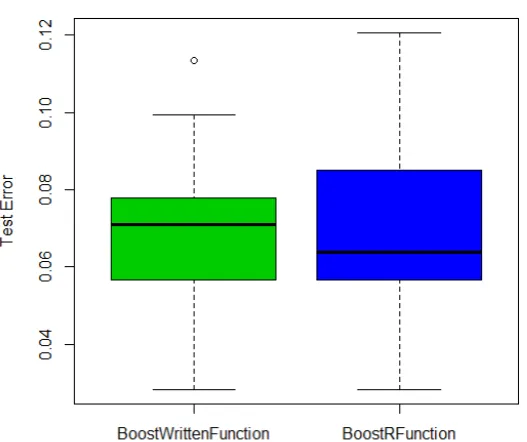
We ran T = 50 iterations of adaptive boosting using each function on the dataset Ionosphere, and saved the test error that each method gener-ated (Sigillito, 1989). The results were nearly always the same or close. In fact, the mean difference between the two functions over each iteration is

0.00014. The average test error results of the50iterations for the R function

and Fokoue, 2015b’s written function were 0.06964539 and 0.06950355, re-spectively. Also, Figure 1.1 shows the distribution of the training error from all iterations of each boosting function with the number of base trees set to

50. Again, since they yield very similar results, and theboosted.trees()

function is more efficient, we have made the decision to use that boosting function (Fokoue, 2015b).

[image:16.595.173.437.405.626.2]

(17)

1.3

The Main Focus

In Chapter 2, we will explain and prove the Training Error Bound Theorem in terms of Schapire and Freund, 2012, which is characterized in the form of:

Pr i∼D1

[H(xi)6=yi]₆ T

Y

t=1

p

1−4γ2

t 6exp −2

T

X

t=1

γ_t2 !

.

wherePri∼D1[H(xi)6=yi]is the specific empirical risk function for the

boosting algorithm equal toR1(H)and H is the chosen function/model.

(18)

Chapter 2

Error Analysis for Adaptive

Boosting

2.1

Training Error Bound

Adaptive Boosting is known to improve data quality because the algorithm was strategically created to choose the more difficult data points to be in the training set. As discussed previously, the points associated with a larger weight are the points that are continually misclassified, so, as a result, those points have a greater chance of being selected to be in the training set (Ab-ney, Schapire, and Singer, 1999). Because of this, the data becomes trained rather quickly, without compromising on accuracy (Appel et al., 2013; Drucker, Schapire, and Simard, 1993). This brings us to the training error bound.

(19)

Chapter 2. Error Analysis for Adaptive Boosting

The Training Bound for Boosting Theorem, as stated by Schapire and Freund, 2012, is the following:

Theorem 2 (Training Error Bound for Boosting). Given the notation for the boosting algorithm stated in Algorithm 1 and Section 1.2.1, letγt=˙ 1₂ −t, and let

D1 be an arbitrary initial distribution over the training set. Then the weighted training error of the combined classifier H with respect toD1 is bounded as:

Pr i∼D1

[H(xi)6=yi]₆ T

Y

t=1

p

1−4γ2

t 6exp −2

T

X

t=1

γ_t2 !

.

Note: γtis always positive becauset 6 1₂.

Proof. Recall the following are defined as:

• Training data: Dn={(xi, yi) :xiX, yi{−1,+1}, i= 1,2, . . . , n}.

• Weak learners: ht(x)fort= 1,2, . . . , T :X → {−1,+1}.

• Initialized weights: D1(i) = 1_n fori= 1,2, . . . , n.

• Choosehtsuch that the error is minimized.

• Chooseαt= 1₂log 1−_tt.

• Update fori= 1,2, . . . , n,

Dt+1 =

Dt(i)

Zt

∗

(

eαt_, _if_h

t(xi) = yi

e−αt_, _if_h

t(xi)6=yi

,

meaning that

Dt+1 =

Zt

,

whereZtis a normalization factor chosen so thatDt+1is a distribution. The final output is

H(x) =sign

T

X

t=1

αtht(x)

! .

• LetF(x) = PT

(20)

Expanding the equation forDT+1 over the occurrences up toT + 1in terms ofDt, we get:

DT+1(i) =D1(i)×

exp −α1yih1(xi)

Z1

× exp −α2yih2(xi)

Z2

×. . .

· · · ×exp −αTyihT(xi)

ZT

= D1(i) exp −yi

PT

t=1αtht(xi)

QT

t=1Zt

= D1(i) exp −yiF(xi)

QT

t=1Zt

.

Recall thatH(x) =sign F(x).

So, ifH(x)6=y, thenyF(x)₆0.

This means thate−yF(x) _>1.

It follows that1{H(X)6=y}₆e−yF(x)_,

meaning1is less than the exponential of−yF(x),given that the response is wrongly classified.

Now, the weighted training error becomes:

Pr i∼D1

[H(xi)6=yi] = n

X

i=1

D1(i)1{H(xi)6=yi}6 n

X

i=1

D1(i) exp −yiF(xi)

= n

X

i=1

DT+1(i)

T

Y

t=1

Zt.

SinceDT+1is a distribution,

Pn

i=1DT+1(i) = 1. Thus,

n

X

i=1

DT+1(i)

T

Y

t=1

Zt = T

Y

t=1

(21)

SinceDt+1 =

Zt andZtis the normalizing factor,Ztmust

make the following true:

Pn

i=1Dt(i) exp −αtyiht(xi)

zt

= 1.

Therefore,

Zt= n

X

i=1

.

Since bothyi andht(xi)take on the values{−1,+1}, whenhtmisclassifies,

yiht(xi) =−1,and when it correctly classifies,yiht(xi) = +1.Therefore, we

can break the above equation down to:

zt=

X

i:yi=hi(xi)

Dt(i)e−αt +

X

i:yi6=hi(xi)

Dt(i)eαt.

The second part of this equation can be recognized as the error multiplied byeαt_{, and the first part is}₁_{minus the error multiplied by}_e−αt_{, so it}

simplifies to:

zt =e−αt(1−t) +eαtt.

And we know thatt = 1₂ −γt, so it follows that

zt=e−αt

1

2 +γt

+eαt1

2 −γt

.

Since we are strategically takingαt= 1₂log1−_tt, the above equation

simplifies to:

e−12log 1−_t

t 1

2+γt

+e12log 1−_t

t 1

2 −γt

.

Again, from the fact thatt= 1₂ −γt, we can write

zt =

1 2 +γt 1 2 −γt

!−1₂

1 2 +γt

+

1 2 +γt 1 2 −γt

!1₂

1 2 −γt

=

1 2 −γt 1 2 +γt

!1₂

1 2 +γt

+

1 2 +γt 1 2 −γt

!1₂

1 2−γt

(22)

=

1 2−γt

1₂

1 2+γt

1₂

+

1 2+γt

1₂

1 2 −γt

1₂

=

1 2−γt

1 2+γt

1₂

+

1 2+γt

1 2−γt

1₂

= 2

1 2−γt

1 2+γt

1₂

2

1

4−γ

2 t 1₂ = 2 r 1

4−γ

2

t =

r

4 1

4−γ

2

t

=p1−4γ2

t.

Now, we have proven thatPri∼D1[H(xi)6=yi]6

QT

t=1

p

1−4γ2

t.

Next, we must prove that

Pr i∼D1

[H(xi)6=yi]6 T

Y

t=1

p

1−4γ2

t 6exp

−2 T

X

t=1

γ_t2

, for anyγ >0.

We start by applying the following approximation:

1 +x₆exfor all realx.

We must show that the condition:

t 6 1

2 −γforγ >0for eacht th

round,

implies the following inequality:

p

1−4γ2

t T

6e−2γ2T.

Since we know that1 +x₆ex_{, if we set}_x₌₋₂_γ2

t,then for eachγi for

i {1,2, . . . , T},it follows that1−2γ_t2 ₆e−2γ2t. This holds because all

γi ∈ R,fori {1,2, . . . , T}. Now, since we are dealing with positive

quantities, we have the following:

q

(1−2γ2

t)2 6e

−2γ2

t →p₁−₄_γ2

t + 4γt4 6e

−2γ2

t_.

Sinceγt >0, we can say that

p

1−4γ2

t 6

p

1−4γ2

t + 4γt4 6e

(23)

Therefore,p1−4γ2

t 6e−2γ

2

t.

Since this holds true for each individualγi, it also holds for the sums over

alli 1,2, . . . , T.

Hence, we can writeQT

t=1

p

1−4γ2

t 6

QT

t=1e

−2γ2

t.

Lastly, this simplifies toQT t=1

p

1−4γ2

t 6e(−2

PT t=1γt2).

We can conclude, then, that

Pr i∼D1

[H(xi)6=yi]6 T

Y

t=1

p

1−4γ2

t 6exp

−2 T

X

t=1

γ_t2

.

(Schapire and Freund, 2012).

We can see now that the training error bound has a decreasing exponen-tial shape. Should we expect the generalized error to take that same form? In Section 2.2, we will show the boosting test and training error plots for10

real datasets. These plots will suggest that the generalized error doeshave the same decreasing exponential form as the training error.

2.2

Empirical Demonstration of the Training

Er-ror

Using 10 datasets of various dimensions, we will run100 iterations of the boosting function to have an empirical look at how the test and training error behave when ranging the number of base trees from1 to50. The 10

datasets analyzed are the following:

• Ionosphere (Sigillito, 1989)

• Breast Cancer (Lichman, 2013b)

(24)

• Dermatology (Lichman, 2013a)

• Letter Recognition (Slate, 1998)

• Colon Cancer (Alon et al., 1999)

• Lung Cancer (Institute, 2016)

• Lymphoma (Fokoue, 2016a)

• Lymphoma 2 (Fokoue, 2016a)

• Prostate Cancer (Fokoue, 2016b)

The lymphoma dataset was subset in two separate ways to create two datasets, which we call Lymphoma, and Lymphoma 2.

The first5datasets on the list are ones with the sample size larger than the number of parameters, denoted by n > p, and the second 5 datasets are ones with a larger number of parameters than sample size, denoted by

p > n(see Table 2.1).

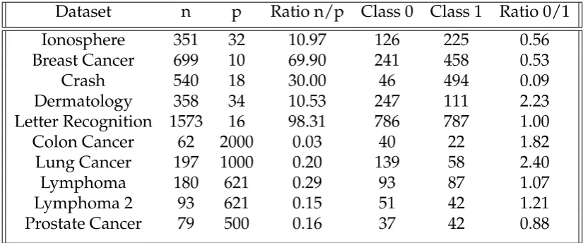
Table 2.1 shows the dimensions of each dataset analyzed, as well as the balance of the response classes. The reason we chose to note these character-istics of the datasets is because datasets with a large number of parameters and small sample sizes tend to be more unstable, thus yielding a larger er-ror. Also, Mazurowskia et al., 2008 found that the error tends to increase when the classes are imbalanced in the training set. What we mean by class imbalance is the response in the training set having more data classified as one group over another. An example of this would be if a training set had more data being classified as 0 than 1. In this case, the model will have more information on Class0, and the out-of-sample predictions might gen-erate more Class0than Class1. If the actual response happens to be more commonly Class1, then there will be a higher rate of misclassification, and thus a higher test error (Mazurowskia et al., 2008) (For more information on addressing the issue of imbalanced classes, see Longadge, Dongre, and Malik, 2013).

(25)

Dataset n p Ratio n/p Class 0 Class 1 Ratio 0/1

Ionosphere 351 32 10.97 126 225 0.56

Breast Cancer 699 10 69.90 241 458 0.53

Crash 540 18 30.00 46 494 0.09

Dermatology 358 34 10.53 247 111 2.23

Letter Recognition 1573 16 98.31 786 787 1.00

Colon Cancer 62 2000 0.03 40 22 1.82

Lung Cancer 197 1000 0.20 139 58 2.40

Lymphoma 180 621 0.29 93 87 1.07

Lymphoma 2 93 621 0.15 51 42 1.21

Prostate Cancer 79 500 0.16 37 42 0.88

TABLE2.1: Dimensions and Class Balance/Imbalance for the

Various Datasets

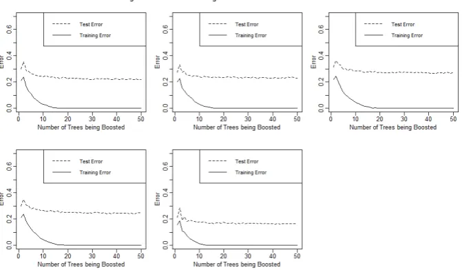
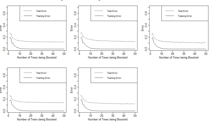
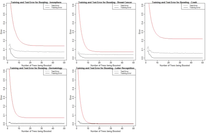
Does it have the same decreasing exponential form as the training error? The error results for the10datasets are shown in Figures 2.1 and 2.2.

The first noticeable aspect of the results is that the error flattens out rel-atively quickly in all cases. What this means for the boosting algorithm is that we do not need to select a large number of trees to boost to get an accu-rate result. In both Figures 2.1 and 2.2, we can see the training and test error begin to flatten aroundT = 20trees. This means that whether we boost 20

or50trees, we are going to get very similar error results. It is better to use fewer trees for the sake of memory usage and efficiency. On the other hand, if one wanted to be as accurate as possible and was not worried about the amount of time it takes the code to run, he or she could use50trees because, with boosting, we do not have to be concerned about over fitting our data (Margineantu and Dietterich, 1997; Schapire, 1999).

Next, it is interesting to note that the test error does have a similar de-creasing exponential shape as the training error (Schapire and Singer, 1999). This is evidence that we will be able to model a generalized bound similar to the Vapnik and Chervonenkis bound in Theorem 1. We are speculating that our bound will be of the form:

R(H)₆Rˆn(H) +φ(. . .)

[image:25.595.112.525.111.283.2]

(26)

difference between the theoretical risk and empirical risk. Since the empiri-cal risk, or training error, plateaus at0, all we must do to model the differ-ence, is model the test error. That brings us to the question: What causes the test error to be larger in some datasets in comparison to others? In Chapter 3, we will share some conjectures inspired by the empirical demonstrations that may answer our question.

FIGURE 2.1: Training and Test Error on Large n Small p

(27)

FIGURE 2.2: Training and Test Error on Large p Small n Datasets

2.3

Existing Bounds

In this section we will state some existing generalized error bounds that are highly sophisticated and quite technical. First, we have a generalized error bound from Schapire and Ene, 2006. This bound is as follows:

R(H)₆Rˆn(H) +O

s

T log|H|+T log n T + log

1

η

n

! .

In this equation,H,T, andnare defined as in Algorithm 1, andηis defined as in Theorem 1. This bound is quite involved and contains many different factors (For more information on this bound, see Schapire and Ene, 2006).

The next bound is one by Vaughan et al., 2006. This bound is defined as:

R(H)₆Rˆn(H) + ˜O

r T ζ

n !

.

(28)

Lastly, Koltchinskii, Panchenko, and Lozano, 2001 have a paper on a generalized error bound, as well. This bound is the most complex of the bounds listed in this section. Koltchinskii, Panchenko, and Lozano, 2001 derive bounds using the VC dimension, and other calculated constants that may be difficult to comprehend (For more information on this bound and to see it stated explicitly, see Koltchinskii, Panchenko, and Lozano, 2001, Section 2).

(29)

Chapter 3

Empirical Demonstration of the

form of Generalization Error of

Boosting

3.1

Conjectures Gathered from Real Datasets

In reference to Figures 2.1 and 2.2, we can now discuss conjectures we have about which characteristics of our dataset, if any, are affecting our test error results. First, we note, in general, how much larger the test error is in the cases with large p small n datasets versus the small p large n datasets. Since all of the graphs are plotted on the same scale, we can easily see that the test error in Figure 2.2 is generally greater than that in Figure 2.1. The datasets in Figure 2.2 that stand out are the Colon Cancer and Prostate Cancer datasets (Alon et al., 1999; Fokoue, 2016b). These two dataset yield the largest test error out of all of the datasets tested. Referring back to Table 2.1, we can see that the Colon Cancer and Prostate Cancer datasets have the smallest sample sizes out of all of the datasets at 62 and 79, respectively. On the contrary, looking at Figure 2.1 we can see that the Letter Recognition dataset clearly has the smallest test error (Slate, 1998). This is the dataset with the largest sample size that was tested, at 1573 observations, it is more than double the sample size of the second largest dataset tested.

(30)

Chapter 3. Empirical Demonstration of the form of Generalization Error of Boosting

test error to the Letter Recognition dataset. From the previous conjecture, we would assume that the sample size for the Dermatology dataset must be relatively large, but in reality, it is not. This dataset has 358 observations, one of the smallest sample sizes in the n > p category. From our general results, it appears that sample size is an important factor in what affects test error, but this leads us to believe something else must also play a crucial role.

Perhaps the number of parameters could also affect the test error. We took subsets of the Lymphoma dataset to create two differentp > ndatasets. We can then directly compare the results of two datasets since they have the same number of parameters but different sample sizes (Fokoue, 2016a). (Note: We may only be able to generalize this to p > n datasets). From Figure 2.2, it seems as though the Lymphoma 2 dataset yields a larger er-ror than the first Lymphoma dataset. The only difference in dimensions is the sample size. Lymphoma 2 has a sample size of93, whereas Lymphoma (yielding a smaller test error) has a sample size of 180, almost double that of Lymphoma 2. Also, as previously stated, the Colon Cancer Dataset and Prostate Cancer dataset both have extremely small sample sizes, but their number of parameters differ greatly with Colon Cancer having2000 param-eters and Prostate Cancer having 500. Although both datasets yield a rel-atively large test error, the Prostate Cancer dataset’s test error is evidently larger than the Colon Cancer dataset’s test error. This may suggest that the greater the number of parameters, the lower the error. We cannot make any conclusions just yet, but this is a good place to start.

(31)

error of thep > ndatasets. The Lymphoma 2 and Prostate Cancer datasets both have a similar ratio of slight imbalance (with one slightly over 1and the other slightly under), yet they produce very different test error results. This leads us to believe that if class imbalance is important, its results may vary based on the previous factors mentioned, or even the ratio of n to p, which is also displayed in Table 2.1. Lastly, the ratio of Class0to Class1in the Dermatology dataset and the Prostate Cancer dataset are very similar at

2.23and 2.40, respectively. Their results are also interesting because, even

though the Dermatology dataset hasn > pand the Prostate Cancer dataset hasp > n, they both yield some of the lowest test error results of the other4

datasets in their respective categories.

In conclusion, it is apparent that sample size, number of parameters, and class imbalance are important factors in the test error outcome but how and in what way, cannot be defined in a simple rule that applies to all datasets. This does, however, give us enough information to simulate multiple datasets of varying sizes for the purpose of applying the boosting algorithm in the same matter as earlier. Since we have evidence that the generalized error of the adaptive boosting algorithm will have the same de-creasing exponential shape as the training error, we will derive a multiple linear regression model,φ, using these mentioned factors as the parameters with the averaged test error as the response. The function φ will then be added to our empirical risk to create a theoretical risk bound similar to the VC Bound in Theorem 1.

3.2

Simulated Datasets

Since the existing bounds discussed in Section 2.3 are too technical and so-phisticated for use in this study, we will go on to create strategically simu-lated datasets of various characteristics that the empirical demonstration in Figure 2.1, Figure 2.2, and Section 3.1 showed may be affecting the gen-eralized error. Simulated datasets are a good tool to use when analyz-ing a theory or conjecture. In the case of simulated datasets, we know the truth because we created the datasets, they are available in any quan-tity, and we know the format will be exactly how we want it (Observational

(32)

datasets in R. Melnykov, Chen, and Maitra, 2012a use the R function called

simdataset()_{from the}MixSim_{package to simulate datasets (Melnykov,}

Chen, and Maitra, 2012b; Melnykov et al., 2015). Another helpful tool for simulating datasets is the sim.item() function from the psychpackage in R (Revelle, 2006; Revelle, 2015). However, we are using a function created by Ramos, 2016 called simclass(). This function enables us to generate datasets of any dimensions. The underlying relationship between the vari-ables and the response can be seen within the function in Appendix A. We kept this underlying relationship constant for all of the simulated datasets. This relationship could effect our results, so by keeping it constant here, we are able to attribute the changes in our results to only the characteristics we are purposly changing. Ramos, 2016’s function uses the calculated response as a probability in the random binomial R function,rbinom()to make the response either a1or0to give us our binary response (R, 1993b).

The idea in this chapter is to take what we learned from our empirical test error results and simulate datasets to test our conjectures. We will study a range of:

• Sample size

• Number of parameters

• Class imbalance/balance

to strategically construct simulated datasets. We will apply the adaptive boosting algorithm to each dataset, ranging the number of trees from 1 to

50and replicate that100times. The results can be seen in Section 3.3, where

there is an analysis of the test and training error plots.

3.2.1

Creating Imbalanced Simulated Datasets

We began by using Ramos, 2016’s function called simclass() _and

con-structed5datasets of each of the varying sizes and dimensions given by:

• n= 250,p= 17

• n= 80,p= 17

(33)

• n= 80,p= 1200

The largest sample size we chose to work with is250, while the smallest is

80. We did not want to construct datasets that were much too large for the

machine to handle, and a sample size of250compared to80should show the contrast in results that we are looking for without it being

unmanageable. Also, the largest number of parameters we chose to

simulate is1200while the smallest is17. This is a large range and seems to be realistic based on the real datasets we were working with. Since we simulated5of each size and dimension, we now have20datasets, and as seen from the list,10of these datasets are of the type small p large n, and the other10data sets are of the type large p small n.

It became apparent that, by default, this function yields an imbalanced class result, meaning the number of data points in Class0was much smaller than the number of data points in Class 1. In fact, the ratio of data points in our datasets classified as Class 0 to those classified as Class 1 ranged anywhere from 0.20 to 0.60. One conjecture discussed is that the ratio of data points in Class 0to those in Class 1 could alter our test error results, so we altered the function to create datasets with a balanced response, as well (i.e., the ratio of Class 0to Class 1 is exactly1). This function, called

simclasseven(), can also be found in Appendix A. We then used this

altered function to create 20 more datasets of the same varying size and dimension as the previous20datasets.

3.2.2

Creating Balanced Simulated Datasets

The way we generatedsimclasseven()came directly from Ramos, 2016’s simulation functionsimclass(). The reasonsimclass()was returning imbalanced results is because it uses the R functionrbinom()to calculate the response of our simulated data (R, 1993b; Ramos, 2016). We altered the code to use the R function median() to calculate the response (R, 1993a). This way, the function takes the calculated relationship between the vari-ables and the response pii _{and classifies anything below the median of} pii _as 0 and anything above the median as 1. Now, we have a balanced

(34)

Next, we will apply the adaptive boosting algorithm to each of the 40

simulated datasets, ranging the number of trees from1to50and replicating that 100 times. The results can be seen in Figures 3.1 through 3.8, and the trends will be discussed in Section 3.3.

FIGURE 3.1: Training and Test Error on Imbalanced Datasets

[image:34.595.144.480.197.393.2]

(35)

of Size 80 X 17

(36)

(37)

3.3

Trends

The results for the imbalanced datasets of the sizes250 X 17, 80X17, 250 X

1200, and80X1200can be found in Figures 3.1, 3.2, 3.3, and 3.4, respectively; the results of these four sizes ofbalanceddatasets are in Figures 3.5, 3.6, 3.7, and 3.8, respectively.

We can see many trends in each of these figures, including the following:

• The datasets of size250X17in Figures 3.1 and 3.5 have a smaller test error than the others.

• The test error varies greatly in the datasets with a sample size of80.

• Some of the datasets with the same attributes yield different results. In regards to the last bullet point, reference Figure 3.2. The second graph (in the middle of the top row) shows a smaller error than the other graphs. This is very interesting because the5plots in this figure come from datasets with the same characteristics, so it is important to note the variability among datasets. These findings for the simulated datasets may help to explain later results; however, our conclusions will be drawn from the Multiple Linear Regression that will be done in Section 3.4.

[image:37.595.144.480.483.678.2]

(38)

FIGURE 3.6: Training and Test Error on Balanced Datasets of Size 80 X 17

FIGURE 3.7: Training and Test Error on Balanced Datasets of

(39)

(40)

3.4

Modeling the Test Error

3.4.1

The Variables

Now we will perform Regression Analysis on the simulated datasets. The data we are using to build this model come directly from the simulated datasets. Our response will be the average test error of each dataset after the "elbow," or after the error begins to flatten. To calculate this response value, we are averaging the mean errors over20replications of the boosting process explained at the end of Section 3.2. For these 20 replications, we only studied the number of trees up toT = 30. As mentioned in Section 2.2, it is evident that the test and training error flatten out closer toT = 20, so instead of requiring much more time and memory to boost the trees until

T = 50, we stopped at T = 30 for these replications. Thus, the response

variable we are using for this Regression Analysis is the average test error of each simulated dataset over all 20replications, from T = 20 toT = 30. The explanatory variables also come from each of the simulated datasets; they are as follows:

• Sample Size, denoted asn

• Number of Parameters, denoted asp

• Ratio of Sample Size to Number of Parameters, denoted asnp

• Number of Data Points in Class0, denoted asz

• Number of Data Points in Class1, denoted aso

• Ratio of Data Points in Class0to Data Points in Class1, denoted aszo

Note: Since we use a stratified random sample in the training/test set split, the number of data points in Class0and Class1will be the same for each individual replication.

Our regression model will take the following form:

log(Ys) = β0 +β1Xs1+. . .+βmXsm+s.

(41)

• Ysis the predicted average test error for simulations;

• Xs1throughXsmare the values that themsignificant explanatory

vari-ables take on from simulations;

• β0throughβmare the calculated coefficients for our model;

• sis the error, or noise, of the model for simulations.

3.4.2

Multiple Linear Regression Models

We constructed several Multiple Linear Regression models before choosing the one that would reveal our test error. The four models are listed below:

• Full multiple linear regression (MLR) model on all6parameters

• Bidirectional stepwise regression, using the Bayesian Information Cri-terion (BIC), on the full MLR model

• Full MLR model on all6parameters with a logarithmic transformation on the response

• Bidirectional stepwise regression, using BIC, on the full MLR model with a logarithmic transformation on the response

The model that best fits our data, is the last one, namely the bidirectional stepwise regression on the full MLR model with a logarithmic transforma-tion on the response. Our MLR model based on the simulated data is the following:

log(Ys) =−1.268 + 0.0003683ps−0.009514zs+s

The only significant variables are the number of parameters, p, and the number of data points classified in group 0, z. Also, we can see that the variable z has a greater affect on the test error outcome than the variable

pbecause the coefficient is larger. These are interesting results because, as

(42)

Since this model was derived with a logarithmic transformation on the response, we must exponentiate our model to return the predicted average test error instead of the log of the predicted average test error. Recall from Section 2.2 that we are modeling our test error for each simulation, Ys to

build our functionφ. Thus,φ, for our case can be defined as:

φ(ps, zs) =Ys= exp(−1.268 + 0.0003683ps−0.009514zs+s).

To reiterate,

• Ysis the predicted average test error for simulations;

• psis the number of parameters for simulations;

• zsis the number of data points in class zero for simulations;

• sis the noise of the model for simulations.

Recall that our intent is to use the basis of the Vapnik Chervonenkis bound to create a generalized bound for the theoretical risk of the adaptive boost-ing algorithm in the form of:

R(H)₆Rˆn(H) +φ(. . .).

We now have an estimated model,φ, said to be:

φ(p, z) =Y = exp(−1.268 + 0.0003683p−0.009514z),

and we have bounded the empirical risk by the following decreasing exponential function:

ˆ

Rn(H)6exp

−2 T

X

t=1

γ_t2

.

(43)

R(H)₆exp−2 T

X

t=1

γ_t2+ exp(−1.268 + 0.0003683p−0.009514z).

A benefit of this generalized error bound in comparison to the bounds in Section 2.3 is that the terms in the function φare more comprehensive. We can see from the bound that as the number of parameters increases, we can expect our generalized error to increase as well. In other words, this bound can give more information to one who was interested in collecting data for a study. He or she can calculate what the structure of the data should be to lower the test error bound.

(44)

Chapter 4

Application to Real datasets

In this section, we will apply the generalization bound to the real datasets presented in Section 2.2. Recall that we are estimating our bound to be:

R(H)₆exp−2 T

X

t=1

γ_t2+ exp(−1.268 + 0.0003683p−0.009514z+),

and the real datasets to which we are applying the bound are the following:

• Ionosphere (Sigillito, 1989)

• Breast Cancer (Lichman, 2013b)

• Crash (Lucas et al., 2013)

• Dermatology (Lichman, 2013a)

• Letter Recognition (Slate, 1998)

• Colon Cancer (Alon et al., 1999)

• Lung Cancer (Institute, 2016)

• Lymphoma (Fokoue, 2016a)

• Lymphoma 2 (Fokoue, 2016a)

• Prostate Cancer (Fokoue, 2016b)

(45)

Chapter 4. Application to Real datasets

Keep in mind that this bound is based on the Vapnik Chervonenkis Bound in Section 1.1, so it is probabilistic, and the projected generalization error may not always bound the test error.

FIGURE 4.1: Large n Small p Real Datasets with Generaliza-tion Error Bound

We can see from these figures that in most cases, the generalization er-ror bound is greater than our empirical test error. The one case among our examples where the generalized error fails to bound the test error is in the Prostate Cancer dataset. These results are shown in the bottom middle graph of Figure 4.2.

[image:45.595.142.480.176.395.2]

(46)

Chapter 4. Application to Real datasets

(47)

Chapter 5

Conclusion

5.1

Restating The Problem

The main focus of this thesis is to model the generalized error. As previously stated in Section 1.3, our goal is to be able to suggest a bound for the gen-eralized error of the Boosting Algorithm. We first boosted ten real datasets of different sizes and characteristics with a binary response, and plotted the error from each dataset.

By studying and analyzing the empirical demonstrations of the ten datasets, we gathered some conjectures about which characteristics of the datasets seemed to be causing the changes in test error results. We concluded that it appears that the following characteristics are important:

• Sample size

• Number of parameters

• Ratio of sample size to number of parameters

• Number of data points in Class0

• Number of data points in Class1

• The ratio of data points in Class0to data points in Class1

We strategically simulated datasets by varying the above-listed characteris-tics, so we can collect more information on exactly what alters the test error and by how much.

(48)

Chapter 5. Conclusion

stepwise multiple linear regression of the 6parameters with a logarithmic transformation of the response pointed to two significant variables. The significant variables are the number of parameters in the dataset and the number of observations in the dataset that had an observed classification as Class0.

This model, explicitly stated, is:

φ(p, z) =Y = exp(−1.268 + 0.0003683p−0.009514z+),

where:

• Y is the predicted average test error;

• pis the number of parameters;

• zis the number of data points in class zero;

• is the noise of the model.

After following the basis of the Vapnik Chervonenkis bound in Theo-rem 1, we derived our proposed generalized error bound of the Boosting Algorithm. It is as follows:

R(H)₆exp−2 T

X

t=1

γ_t2+ exp(−1.268 + 0.0003683p−0.009514z+).

5.2

Impact of the Generalized Error Bound

(49)

Chapter 5. Conclusion

number of parameters is going to increase the upper bound of the boosting algorithm’s test error.

5.3

Future Results

If one were inclined to continue research to make this test error bound more accurate, we would suggest simulating more datasets of different sizes. We used 4sizes of data sets: 250 X17, 80X 17, 250 X1200, and80 X1200. We simulated 5datasets of each size with an imbalanced binary response and

5datasets of each size with a balanced binary response. Had we had more

resources, we could have simulated datasets with a larger sample size. The largest sample size of the real datasets that were studied is n = 1573. If a larger range of sample sizes had been covered, we may have been able to get even more generalizable results without extrapolation.

(50)

Appendix A

R Functions

winds <− f u n c t i o n(nrow, ncol, maxsize =6 , aryx =1 ,

cex . l a b = 1 . 2 , cex .a x i s= 1 . 2 , t i t l e=FALSE , mars=c( 3 , 3 . 2 , 1 , 1 ) + . 1 , omas=c( 0 , 0 , 0 , 0 ) ,

mgps=c( 2 , 0 . 7 , 0 ) , m a r 3 t i t l e P l u s =2 , byrow=TRUE)

{

graph . a r <− aryx∗nrow / ncol

i f ( graph . a r > 1 ) { r s i z e <− maxsize ;

c s i z e <− maxsize/graph . a r } e l s e

{ c s i z e <− maxsize ;

r s i z e <− maxsize∗graph . a r } windows ( c s i z e , r s i z e )

i f ( byrow ) par( mfrow=c(nrow, ncol) ) e l s e par( mfcol=c(nrow, ncol) )

par( mar=c( mars [ 1 ] , mars [ 2 ] , i f e l s e(t i t l e , mars [ 3 ] + m a r 3 t i t l e P l u s ,

mars [ 3 ] ) , mars [ 4 ] ) ,

mgp=mgps , oma=i f(length( omas ) = = 1 )

c( 0 , 0 , omas , 0 ) e l s e i f (length( omas ) = = 2 )

c( omas [ 1 ] , 0 , omas [ 2 ] , 0 ) e l s e omas , cex . l a b =cex . lab , cex .a x i s=cex .a x i s)

i n v i s i b l e ( ) }

(51)

Appendix A. R Functions

Y <− xy $Y

n <− nrow(xy)

m <− round( 0 . 7 5∗n ) p <− ncol(xy)−1

T <− nbase

alpha <− numeric( T ) e p s i l o n <− numeric( T ) weight <− rep( 1/n , n )

h <− NULL

f o r(t i n 1 : T ) {

decent . base . l e a r n e r <− 0

while(!decent . base . l e a r n e r ) {

b o o s t . id <− sample( 1 : n , m,

r e p l a c e=T , prob=weight ) base . l e a r n e r <− r p a r t (as . f a c t o r( Y )~. ,

data=xy, subset=b o o s t . i d ) yhat <− p r e d i c t( base . l e a r n e r ,

xy[ ,−( p + 1 ) ] , type= ’ c l a s s ’ ) e p s i l o n . c a n d i d a t e <− e r r o r .weighted( Y ,

yhat , weight )

i f e l s e( e p s i l o n . c a n d i d a t e ==0 ,

e p s i l o n . c a n d i d a t e <− 0 . 0 0 0 1 ,

e p s i l o n . c a n d i d a t e <− e p s i l o n . c a n d i d a t e ) decent . base . l e a r n e r <− ( e p s i l o n . c a n d i d a t e < 0 . 5 ) }

e p s i l o n [t] <− e p s i l o n . c a n d i d a t e

alpha [t] <− ( 1/2 )∗log((1−e p s i l o n [t] ) / e p s i l o n [t ] ) weight <− weight∗exp( alpha [t]∗i n d i c a t o r ( Y! =yhat ) )

weight <− weight/ sum( weight )

(52)

}

r e t u r n(l i s t ( alpha=alpha , h=h , weight=weight ) ) }

p r e d i c t . boosted . t r e e <− f u n c t i o n( h , alpha , xnew ) {

T <− length( h ) nnew <− nrow( xnew ) h . t. x <− NULL

f o r(t i n 1 : T ) { h .t . x <− cbind( h . t. x , pm(p r e d i c t( h [ [ t ] ] , xnew , type= ’ c l a s s ’ ) ) ) }

m. alpha <− matrix(rep( alpha , nnew ) , byrow=T , nrow=nnew )

r e t u r n(i f e l s e( rowSums (m. alpha∗h .t . x ) < 0 . 5 , 0 , 1 ) ) }

e r r o r .weighted <− f u n c t i o n( y , yhat , weight ) {

e r r <− i f e l s e( y! =yhat , 1 , 0 )

r e t u r n(sum( e r r∗weight ) ) }

i n d i c a t o r <− f u n c t i o n( p r e d i c a t e ) {

r e t u r n(i f e l s e( p r e d i c a t e , 1 , 0 ) ) }

pm <− f u n c t i o n( y ) {

uy <− s o r t(unique( y ) )

r e t u r n(i f e l s e( y==uy [ 1 ] ,−1 , + 1 ) ) }

(53)

{

n <− length( l a b e l )

confmat <− t a b l e( l a b e l , response) Accuracy <− sum(diag( confmat ) ) /n

FPR <− confmat [ 1 , 2 ] /rowSums ( confmat ) [ 1 ] TPR <− confmat [ 2 , 2 ] /rowSums ( confmat ) [ 2 ] FNR <− confmat [ 2 , 1 ] /rowSums ( confmat ) [ 2 ] TNR <− confmat [ 1 , 1 ] /rowSums ( confmat ) [ 1 ] P r e c i s i o n <− confmat [ 2 , 2 ] /colSums ( confmat ) [ 2 ]

R e c a l l <− TPR S p e c i f i c i t y <− TNR S e n s i t i v i t y <− TPR

F . measure <− 2∗( P r e c i s i o n∗R e c a l l)/( P r e c i s i o n +R e c a l l) measured <− l i s t ( Accuracy=Accuracy ,

P r e c i s i o n = P r e c i s i o n , F . measure = F . measure ,

R e c a l l=Recall ,

FPR=FPR , TPR = TPR , FNR=FNR, TNR = TNR,

S p e c i f i c i t y = S p e c i f i c i t y , S e n s i t i v i t y = S e n s i t i v i t y )

r e t u r n( measured ) }

e x t r a c t<−f u n c t i o n( measure ) {

v <− numeric( 1 0 )

v [ 1 ] <− measure$Accuracy v [ 2 ] <− measure$P r e c i s i o n v [ 3 ] <− measure$ R e c a l l

v [ 4 ] <− measure$F . measure v [ 5 ] <− measure$FPR

(54)

v [ 9 ] <− measure$S p e c i f i c i t y v [ 1 0 ] <− measure$S e n s i t i v i t y

r e t u r n( v ) }

s i m c l a s s <− f u n c t i o n( n =300 ,p=10 , seed=NULL) {

s e t. seed ( seed )

mu <− round(r u n i f( p , 0 , 1 ) , 2 ) sigma <− round(r u n i f( p , 1 , 3 ) , 2 )

sigma .m <− ‘diag <−‘ (matrix( 0 , p , p ) , 1 )∗sigma X <− mvrnorm ( n , mu, sigma .m)

y <− X [ , 1 ] + X [ , 4 ] + X [ , 5 ] p i i <− 1/(1+exp(−y ) ) y .c <− rbinom( n , 1 , p i i )

t a b l e( y .c)

sim . dat .c <− data.frame(cbind( y .c, X ) )

names( sim . dat .c) [ 1 ] <− "Y"

r e t u r n( sim . dat .c) }

s i m c l a s s e v e n <− f u n c t i o n( n =300 ,p=10 , seed=NULL) {

s e t. seed ( seed )

mu <− round(r u n i f( p , 0 , 1 ) , 2 ) sigma <− round(r u n i f( p , 1 , 3 ) , 2 )

sigma .m <− ‘diag <−‘ (matrix( 0 , p , p ) , 1 )∗sigma X <− mvrnorm ( n , mu, sigma .m)

y <− X [ , 1 ] + X [ , 4 ] + X [ , 5 ] p i i <− 1/(1+exp(−y ) )

y .c <− i f e l s e( p i i <=median( p i i ) , 0 , 1 )

t a b l e( y .c)

sim . dat .c <− data.frame(cbind( y .c, X ) )

names( sim . dat .c) [ 1 ] <− "Y"

(55)

}

(56)

Bibliography

Abney, Steven, Robert Schapire, and Yoram Singer (1999). Boosting Applied

to Tagging and PP Attachment. Tech. rep. Florham Park, NJ: AT&T Labs.

Alfaro, Esteban, Matias Gamez, and Noelia Garcia (2013). “adabag: An R Package for Classification with Boosting and Bagging”. In:Journal of Sta-tistical Software54.2.

Alfaro, Esteban et al. (2015). Package ‘adabag’. URL: https : / / cran . r -project.org/web/packages/adabag/adabag.pdf.

Alfaro-Cortes, Esteban et al. (2016).R Documentation - Applies Multiclass

Ad-aBoost.M1, SAMME and Bagging. URL: http://127.0.0.1:28781/

library/adabag/html/adabag-package.html.

Alon, U. et al. (1999). “Broad Patterns of Gene Expression Revealed by Clus-tering Analysis of Tumor and Normal Colon Tissues Probed by Oligonu-cleotide Arrays”. In:Proceedings of the National Academy of Sciences of the

United States of America96, pp. 6745–6750.

Appel, Ron et al. (2013). Quickly Boosting Decision Trees - Pruning

Under-achieving Features Early. Tech. rep. 28. JMLR Workshop and Conference

Proceedings.

Drucker, Harris and Corinna Cortes (1996). “Boosting Decision Trees”. In:

Advances in Neural Information Processing Systems8.

Drucker, Harris, Robert Schapire, and Partice Simard (1993). “Improving Performance in Neural Networks Using a Boosting Algorithm”. In:

Ad-vances in Neural Information Processing Systems5, pp. 42–49.

Fokoue, Ernest (2015a).Lecture Notes for Principles of Statistical Data Mining. — (2015b). R Code for various Functions. Rochester Institute of Technology

Principles of Data Mining Course.

— (2016a).Lymphoma Dataset. Lymphoma Dataset.

(57)

BIBLIOGRAPHY

Freund, Yoav and Robert E. Schapire (1996).Experiments with a New

Boost-ing Algorithm. Paper presented at Machine Learning: Proceedings of the

Thirteenth International Conference. Murray Hill: AT&T Laboratories. Institute, Broad (2016). Cancer Program Legacy Publication Resources - Lung

Cancer Data. URL: http://www.broadinstitute.org/cgi- bin/

cancer/publications/view/87.

James, Gareth et al. (2013).An Introduction to Statistical Learning with

Appli-cations in R. New York: Springer Science+Business Media.

Koltchinskii, Vladimir, Dmitriy Panchenko, and Fernando Lozano (2001). “Some New Bounds on the Generalization Error of Combined Classi-fiers”. MA thesis. University of New Mexico.

Kuhn, Max (2015). A Short Introduction to the Caret Package. URL: https : / / cran . r - project . org / web / packages / caret / vignettes /

caret.pdf.

Lichman, M. (2013a).UCI Machine Learning Repository - Dermatology Data Set.

URL:http://archive.ics.uci.edu/ml/datasets/Dermatology. — (2013b). UCI Machine Learning Repository – Breast Cancer Data Set. URL:

http://archive.ics.uci.edu/ml/datasets/Dermatology_.

Loh, Wei yin (2011). “Classification and Regression Trees”. In: Wiley

Inter-disciplinary Reviews: Data Mining and Knowledge Discovery, pp. 14–23.

Longadge, Rushi, Snehlata S. Dongre, and Latesh Malik (2013). “Class Im-balance Problem in Data Mining: Review”. In: International Journal of

Computer Science ad Network2.1.

Lucas, D. et al. (2013). “Failure Analysis of Parameter-Induced Simulation Crashes in Climate Models”. In:Geoscientific Model Development, pp. 585– 623.

Margineantu, Dragos D. and Thomas G. Dietterich (1997).Pruning Adaptive

Boosting. Tech. rep. Oregon State University.

Mazurowskia, Maciej A. et al. (2008). “Training Neural Network Classifiers for Medical Decision Making: The Effects of Imbalanced Datasets on Classification Performance”. In:Neural Networks21.2-3, pp. 427–436. Melnykov, Volodymyr, Wei-Chen Chen, and Ranjan Maitra (2012a). “MixSim:

(58)

BIBLIOGRAPHY

Melnykov, Volodymyr, Wei-Chen Chen, and Ranjan Maitra (2012b).

sim-dataset.URL:http://finzi.psych.upenn.edu/library/MixSim/

html/simdataset.html.

Melnykov, Volodymyr et al. (2015). MixSim: Simulating Data to Study

Per-formance of Clustering Algorithms. URL: https://cran.r- project.

org/web/packages/MixSim/index.html.

Observational Medical Outcomes Partnerships (2013). URL: http : / / omop .

org/node/70.

Ohio, State University (2015). Boosting. URL: http : / / www . stat . osu . edu/~yklee/boosting.pdf_.

Quinlan, J. Ross (2006).Bagging, Boosting, and C4.5. Paper presented at Pro-ceedings, Forteenth National Conference on Artficial Intellegence. Syd-ney: University of Sydney.

R, Team Core (1993a).Median Value. URL: https://stat.ethz.ch/R-manual/R-devel/library/stats/html/median.html.

— (1993b).The Binomial Distribution. URL: https://stat.ethz.ch/R-manual/R-devel/library/stats/html/Binomial.html.

— (2016).R: A Language and Environment for Statistical Computing. http://www.R-project.org/. R Foundation for Statistical Computing.

Ramos, Andre Lobato (2016).Simulating Data Code.

Revelle, William (2006).Generate simulated data structures for circumplex,

spher-ical, or simple structure. URL: http://www.personality- project.

org/r/html/sim.item.html.

— (2015).Procedures for Psychological, Psychometric, and Personality Research.

URL: https : / / cran . r - project . org / web / packages / psych / psych.pdf.

Sarkar, Deepayan (2015). Trellis Graphics for R. URL: https : / / cran . r -project.org/web/packages/lattice/lattice.pdf_.

Schapire, Rob and Alina Ene (2006).Foundations of Machine Learning Lecture 10.

Schapire, Robert and Yoram Singer (1999). “Improved Boosting Algorithms Using Confidence-rated Predictions”. In: Machine Learning37, pp. 297– 336.

— (2000). “BoosTexter: A Boosting-based System for Text Categorization”.

(59)

BIBLIOGRAPHY

Schapire, Robert E. (1999). “A Brief Introduction to Boosting”. In:Conference on Artificial Intellegence. AT&T Labs, pp. 1–6.

Schapire, Robert E. and Yoav Freund (2012). Adaptive Computation and

Ma-chine Learning : Boosting : Foundations and Algorithms. Cambridge: MIT

Press.

Sigillito, Vince (1989). R Documentation Johns Hopkins University Ionosphere

database. URL: http : / / 127 . 0 . 0 . 1 : 28781 / library / mlbench /

html/Ionosphere.html.

Slate, David (1998).R Documentation Letter Image Recognition Data.URL:http: //127.0.0.1:15163/library/mlbench/html/LetterRecognition.

html_.

Therneau, Terry, Beth Atkinson, and Brian Ripley (2015).Recursive

Partition-ing and Regression Trees. URL:https://cran.r-project.org/web/

packages/rpart/rpart.pdf.

Touloumis, Anestis (2015).Shrinkage Covariance Matrix Estimators.URL:https:

//cran.r-project.org/web/packages/ShrinkCovMat/ShrinkCovMat.

pdf.

Vaughan, Jennifer Wortman et al. (2006).Machine Learning Theory Lecture 14: Generalization Error of Adaboost.

Theses

Thesis/Dissertation Collections

ROCHESTER

Paige HOUSTON

Dr. Ernest FOKOUÉ

School of Mathematical Sciences

College of Science

ROCHESTER INSTITUTE OF TECHNOLOGY

Ernest Fokoué

https : / / cran . r

-project.org/web/packages/adabag/adabag.pdf

.

http://127.0.0.1:28781/library/adabag/html/adabag-package.html

http://www.broadinstitute.org/cgi- bin/cancer/publications/view/87

https :/ / cran . r - project . org / web / packages / caret / vignettes /

http://archive.ics.uci.edu/ml/datasets/Dermatology.

http://finzi.psych.upenn.edu/library/MixSim/html/simdataset.html

https://cran.r- project.org/web/packages/MixSim/index.html

http : / / omop .org/node/70

http : / / www . stat . osu .edu/~yklee/boosting.pdf

An Empirical Demonstration of the Probabilistic Upper Bound of the Adaptive Boosting Test Error

Rochester Institute of Technology

OCHESTER

School of Mathematical Sciences

Committee Approval Form

ROCHESTER INSTITUTE OF TECHNOLOGY

Abstract

An Empirical Demonstration of the Probabilistic Upper Bound of the Adaptive Boosting Test Error

Contents

Declaration of Authorship i

5 Conclusion 39

List of Figures

Chapter 1

Vapnik and Chervonenkis Bound

Adaptive Boosting

The Algorithm

The Boosting Function in R

The Main Focus

Chapter 2

Empirical Demonstration of the Training

Existing Bounds

Chapter 3

Simulated Datasets

Creating Imbalanced Simulated Datasets

Creating Balanced Simulated Datasets

Trends

Modeling the Test Error

Multiple Linear Regression Models

Chapter 4

Chapter 5

Impact of the Generalized Error Bound

Appendix A

FPR=FPR , TPR = TPR , FNR=FNR, TNR = TNR,

Bibliography

BIBLIOGRAPHY

BIBLIOGRAPHY

BIBLIOGRAPHY