Balancing truth error and manual processing in the PDQ system

(1)

Theses Thesis/Dissertation Collections

2011

Balancing truth error and manual processing in the

PDQ system

Douglass Huang

Follow this and additional works at:http://scholarworks.rit.edu/theses

This Thesis is brought to you for free and open access by the Thesis/Dissertation Collections at RIT Scholar Works. It has been accepted for inclusion in Theses by an authorized administrator of RIT Scholar Works. For more information, please [email protected].

Recommended Citation

(2)

by

Douglass Huang

A Thesis Submitted in Partial Fulfillment of the Requirements for the Degree of Master of Science

in Computer Science

Supervised by

Professor Roger S. Gaborski, Ph.D. Department of Computer Science

B. Thomas Golisano College of Computing and Information Sciences Rochester Institute of Technology

Rochester, New York August 25, 2011

Approved by:

Roger S. Gaborski, Ph.D., Professor

Thesis Advisor, Department of Computer Science

Peter G. Anderson, Ph.D., Professor Emeritus

Committee Member, Department of Computer Science

K. Bradley Paxton, Ph.D., CEO

(3)

Rochester Institute of Technology

B. Thomas Golisano College of Computing and Information Sciences

Title:

Balancing Truth Error and Manual Processing in the PDQ System

I, Douglass Huang, hereby grant permission to the Wallace Memorial Library to reproduce my thesis in whole or part.

Douglass Huang

(4)

Dedication

(5)

Acknowledgments

I am grateful to the following people for all their support, patience, and encouragement: my wife, Mrs. Nina Huang; my parents, Dr. Ji-Ming Huang and Mrs. Chuei-Yun Huang; my committee members, Dr. Roger

(6)

Abstract

Balancing Truth Error and Manual Processing in the PDQ System

Douglass Huang

Supervising Professor: Roger S. Gaborski, Ph.D.

Production Data Quality (PDQ) is a specialized pattern classifier whose main purpose is to assess independently the data quality of a production classifier. It accomplishes this by producing a high quality Truth from the source input, and then using the Truth to identify errors in the production classifier’s output data. Previous studies have shown close agreement be-tween PDQ processing outcomes and a particular mathematical model of the system.

In this study we describe and analyze an expanded model that addresses the potential tradeoff between Truth error and manual processing in PDQ, with an eye towards informing operational decisions about precision and efficiency. Using statistical data from the 2010 Census PDQ system as input, we examine the predictions of the new model in order to understand their potential usefulness.

(7)

List of Tables

3.1 Path Predictor: Y(θ)[y, z(θ)] . . . 14

5.1 Results for total sample: Static model. . . 33

5.2 Results through Week 3 of May 2010: Static model. . . 51

5.3 Results through Week 3 of May 2010: Tuning values. . . 51

(10)

List of Figures

2.1 PDQ Process Flow: Main components. . . 4

2.2 PDQ Process Flow: Arbitrator steps. . . 6

2.3 PDQ Process Flow: Independent Data Capture steps. . . 9

3.1 Expanded PDQ Model: Projector steps. . . 13

5.1 Results for total sample: Components of minimum Pro-jected Truth error rate: Method 1 (minE1T(θ)). . . 35

5.2 Results for total sample: Components of maximum Pro-jected Truth error rate: Method 1 (maxE1_T(_θ₎). . . 36

5.3 Results for total sample: Comparison of minimum and max-imum Projected Truth error rates: Method 1 (minE1T(θ) and maxE1T(θ)). . . 37

5.4 Results for total sample: Components of Projected Provi-sional Truth error rate (EPT(θ)). . . 38

5.5 Results for total sample: Comparison of minimum and max-imum Projected Truth error rates: Method 2 (minE2_T(_θ₎ and maxE2T(θ)). . . 39

5.6 Results for total sample: Comparison of projected error rates (Ex). . . 41

5.7 Results for total sample: Components of minimum pro-jected manual processing rate (minMT(θ)). . . 42

(11)

5.9 Results for total sample: Comparison of minimum and

max-imum projected manual processing rates (minM_T(_θ₎ and

maxMT(θ)). . . 45

5.10 Results for total sample: Projected Provisional Truth error

rate (EPT(θ)) v. projected reject rate (FK(θ)). . . 46

5.11 Results for total sample: Minimum Projected Truth error

rate: Method 2 (minE2T(θ)) v. maximum projected manual

processing rate (maxMT(θ)). . . 47

5.12 Results for total sample: Comparison of Projected

Pro-visional Truth error rate (EPT(θ)) v. projected reject

rate (FK(θ)) and minimum Projected Truth error rate:

Method 2 (minE2T(θ)) v. maximum projected manual

pro-cessing rate (maxM_T(_θ₎). . . 48 5.13 Results through Week 3 of May 2010: Tuning chart. . . 52

(12)

Chapter 1

Introduction

Production Data Quality (PDQ) [1] is a system developed at ADI, LLC to measure the accuracy of a pattern classifier when processing “produc-tion” inputs, where the true classifications are not known a priori. It can be applied generically in a number of classification domains, such as finger-print matching or record linkage. In one particular instance, PDQ has been used to assess the quality of the Decennial Response Integration System’s (DRIS) [13] electronic capture of handprint and check mark responses on 2010 Census paper forms. In order to make its measurements, PDQ first produced a high quality Truth for a sample of scanned Census form im-ages, using a combination of automated recognition and human processing. Paxton, et al., have described a mathematical model [12] to predict the out-comes of this process based on certain input conditions, and in practice the actual outcomes have agreed very well with the predictions.

PDQ itself is a special case of pattern classifier, and as such, the simplest measure of its performance is the Truth error rate, the fraction of response fields for which it assigns an incorrect Truth value [6]. Because its main purpose is to measure the accuracy of a production classifier system, PDQ’s Truth error rate must be sufficiently low in comparison to the error rate of the production output data. Another useful measure of PDQ’s performance is the manual processing rate, expressed as the fraction of fields that require human review or arbitration to determine the Truth. Reducing this work-load can result in reduced labor costs or increased throughput, but likely additional Truth error.

(13)

(14)

Chapter 2

Supporting Work

2.1

Production Data Quality

2.1.1 Process Flow

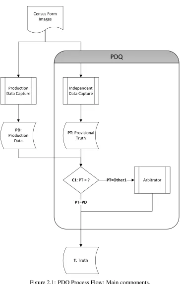
In its 2010 Census embodiment, the PDQ system has the following main components [12, 7], shown in Figure 2.1:

Independent Data Capture system Processes the Census form images and outputs the Provisional Truth (data set PT). This is analogous to the Production Data Capture system, whose Produc-tion Data (data set PD) is being evaluated, but it has been developed independently to meet equivalent input/output specifications.

Comparator 1 (C1) Determines automatically, on a field-by-field basis, whether the response val-ues in the Production Data and Provisional Truth are identical (path PT=PD). Matching values are designated as Truth (data set T) and require no further processing.

Arbitrator Incorporates human analysts to resolve the Truth for any non-matching fields (path PT=Other1) identified by Comparator 1.

2.1.2 Arbitrator

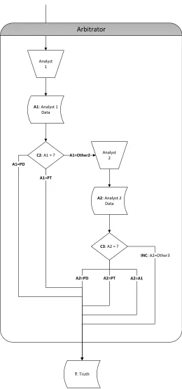
The steps within the Arbitrator, shown in Figure 2.2, are as follows:

Analyst 1 Enters a value for each field sent to the Arbitrator, producing the data set A1.

Comparator 2 (C2) Determines automatically whether Analyst 1’s value matches that of the Pro-duction Data (path A1=PD) or Provisional Truth (path A1=PT). If so, that value is designated as Truth and requires no further processing.

(15)

Census Form Images

Production Data Capture

PD: Production

Data

Independent Data Capture

PT: Provisional Truth

C1: PT = ? Arbitrator

T: Truth PT=PD

PDQ

[image:15.612.128.491.101.674.2]

PT=Other1

(16)

duction Data (path A2=PD), Provisional Truth (path A2=PT), or Analyst 1 (path A2=A1). If so, that value is designated as Truth. Otherwise (path A2=Other3, or INC), PDQ designates the field as Inconclusive.

2.1.3 Static Model

The mathematical model of PDQ given by Paxton,et al.[12], takes as inputs the error rates of four of the data sets identified above. Error rates are defined as follows:

fx≡the number of fields in data setx

ex≡the number of errors in data setx

Ex≡the error rate of data setx

Ex=

ex

fx

(2.1)

The inputs to the model are the following:

EPD ≡the error rate of the Production Data

EPT≡the error rate of the Provisional Truth

EA1≡the error rate of Analyst 1’s output

EA2≡the error rate of Analyst 2’s output

We define the setY as follows:

Y ≡the set of all direct pathsyto the Truth

Y ={PT=PD,A1=PD,A1=PT,A2=PD,A2=PT,A2=A1,INC} (2.2)

(17)

Analyst 1

C2: A1 = ?

T: Truth

Analyst 2

C3: A2 = ? Arbitrator

A1: Analyst 1 Data

A1=Other2

A2=PD A2=PT A2=A1

INC: A2=Other3 A2: Analyst 2

Data A1=PD

[image:17.612.179.439.106.660.2]

A1=PT

(18)

P[y]≡the probability that a field follows pathy

P[PT=PD] = (1−EPD)(1−EPT) (2.3a)

P[A1=PD] = (1−EPD)EPT(1−EA1) (2.3b)

P[A1=PT] =EPD(1−EPT)(1−EA1) (2.3c)

P[A2=PD] = (1−EPD)EPTEA1(1−EA2) (2.3d)

P[A2=PT] =EPD(1−EPT)EA1(1−EA2) (2.3e)

P[A2=A1] =EPDEPT(1−EA1)(1−EA2) (2.3f)

P[INC] =EPDEPT(EA1+EA2) +EA1EA2(EPD+EPT)−3EPDEPTEA1EA2 (2.3g)

X

y∈Y

P[y] = 1 (2.3h)

2.1.4 Truth Error Rate

We define f[y] andF[y]as follows:

f[y]≡the number of fields that follow pathy

F[y]≡the rate at which fields follow pathy

F[y] = f[y]

fT

(2.4)

Paxton [11] gives the following estimate of the PDQ Truth error rateET:

ET = max

y∈Y |F[y]−P[y]| (2.5)

For the purposes of my study, I assume that this is a practical baseline estimate. In one representative subset of 2010 Census results [7], PDQ mea-sured a Production Data error rate of EPD = 0.28%, while the Truth error

rate given by Equation (2.5) was a substantially lower ET = 0.01%,

(19)

2.1.5 Independent Data Capture System

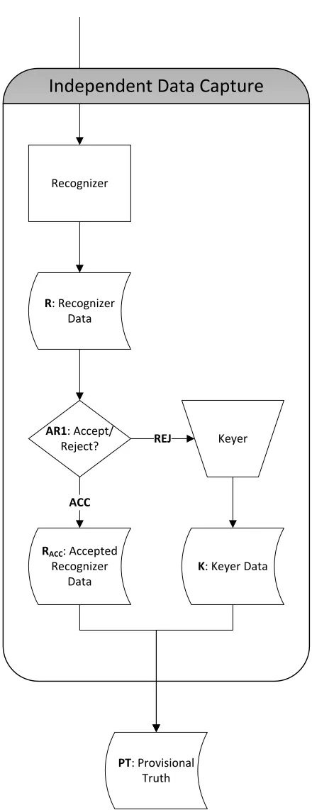
Next, we take a more detailed look at the following steps within the Inde-pendent Data Capture system [12], shown in Figure 2.3:

Recognizer Uses OCR or optical mark recognition (OMR) to assign automatically a response value and an integral confidence level in the range [0,100] for each field on each Census form image, producing the data set R.

Acceptor 1 (AR1) Determines automatically, based on the Recognizer outputs and an integral con-fidence thresholdθ0 ∈ [−1,100], whether the value of each field in data set R isaccepted.

While there are specific exceptions due to complex contextual rules, in general a field is ac-cepted if its confidence levelexceedsθ0. If it is accepted (path ACC), the field contributes to

the data set RACC, which becomes part of the Provisional Truth.

Keyer Performs manual review of each fieldrejected by the Acceptor (path REJ). Enters a value into the data set K, which completes the Provisional Truth data set.

2.1.6 Manual Processing Rate

While the EPT input of the static model reflects one performance measure

of the Independent Data Capture system, it does not account for the reject rate, which reflects the amount of human review required to produce the Provisional Truth. We define the reject rate FK as follows:

Fx ≡the rate at which fields contribute to data setx

Fx =

fx

fT

(2.6)

FK=the reject rate of the Independent Data Capture system

FK=

fK

fT

(2.7)

An analogous performance measure for PDQ as a whole is the manual processing rate [11], which reflects the total amount of human review and arbitration required to determine the Truth. We define the manual process-ing rate MT as follows:

mT ≡the manual processing volume required to determine the Truth

mT =fK+fA1+fA2 (2.8)

MT ≡the manual processing rate required to determine the Truth

MT =

mT

fT

(20)

Recognizer

Independent Data Capture

AR1: Accept/ Reject?

PT: Provisional Truth

Keyer R: Recognizer

Data

RACC: Accepted Recognizer

Data

K: Keyer Data REJ

[image:20.612.199.419.95.666.2]

ACC

(21)

2.2

Error and Manual Processing Tradeoff

The tradeoff between error and reject has been well studied as a means to characterize and optimize the performance of handwriting recognition sys-tems [3, 2]. A typical approach begins with processing a training deck of known truth using an automated recognizer. The recognizer outputs both a response value and an integral confidence level for each work unit. One can then determine the proportion of fields whose confidence levels are below different possible confidence thresholds (reject rate), and also the proportion of incorrect response values among accepted fields (error rate). These kinds of data, especially in conjunction with a cost model [4, 9], can be used to determine optimal confidence thresholds for the system.

The most obvious application in PDQ is to examine how the confidence threshold θ0 within the Independent Data Capture system impacts both the

(22)

Chapter 3

Expanded Model of PDQ Outcomes

PDQ’s main role in the 2010 Census was to verify the DRIS contractor’s ad-herence to certain data quality service-level agreements (SLAs), expressed in terms of the error rate EPD, for specific strata within the Production Data

set. For example, the total write-in fields captured by optical character recognition (OCR) with high confidence were required to haveEPD ≤ 1.0%.

It stands to reason that a certain Truth error rate, perhapsET = 0.1%, would

be sufficiently low for verifying SLA compliance, while an even lower Truth error rate would be unnecessary for that purpose. Because lower Truth error rates typically come at the cost of additional manual processing, it would be helpful to have some control over this tradeoff. I have devised an expanded view of the PDQ processing outcomes that attempts to address this concern.

3.1

Projector

Given some estimate of ET and an observed MT, we wish to predict how

each of these performance measures would change after reducing the confi-dence threshold fromθ0. For this purpose I introduce the Projector, a logical

component that examines the processing outcomes (i.e., data set contents and comparator decisions) from PDQ and computes the projected outcomes for integral confidence thresholds θ, where θ ∈ [−1, θ0]. The case θ = −1

results in acceptance of the most fields possible, while θ = θ0 results in the

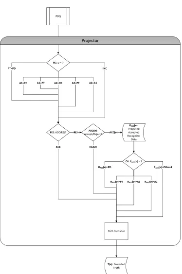
original PDQ outcomes. Figure 3.1 shows the steps within the Projector, which are as follows:

(23)

Path Identifier 2 (PI2) Inspects automatically the decision of Acceptor 1. Fields that were ac-cepted (path ACC) at the original confidence thresholdθ0would be unchanged by applying

a lower threshold. Fields that were rejected (path REJ) require further consideration.

Acceptor 2 (AR2(θ)) Determines automatically whether each field that was previously rejected would be accepted at the new thresholdθ. If there would be no change (path REJ(θ)), then no further analysis is needed. For fields that would be accepted (path ACC(θ))), the original Recognizer values are added to the data set RACC(θ).

Comparator 4 (C4) Determines automatically whether the value for each field in RACC(θ)matches

that from either the Production Data (path RACC(θ)=PD), original Provisional Truth (path

RACC(θ)=PT), Analyst 1 (path RACC(θ)=A1), Analyst 2 (path RACC(θ)=A2), or none of

these (path RACC(θ)=Other4).

Path Predictor Determines automatically the Projected Truth (data set T(θ)) by predicting a new terminal path y(θ) based ony and the incoming pathz(θ) from PI2, AR2(θ), or C4. In certain cases,y(θ)is indeterminate, as described later in Section 3.2.

3.2

Path Predictor

To support the description of the Path Predictor’s function, we define the following:

Z(θ)≡the set of all direct pathsz(θ)to the Path Predictor

Z(θ) ={RACC(θ)=PD,RACC(θ)=PT,RACC(θ)=A1,RACC(θ)=A2,RACC(θ)=Other4}

(3.1)

Y(θ)≡the set of all direct pathsy(θ)to the Projected Truth

Y(θ) =Y ∪ {PT(θ)=PD,A1=PT(θ),A2=PT(θ)} (3.2)

Y(θ)[y, z(θ)]≡the set of pathsy(θ)that are possible for each field that follows the pathsyand

z(θ)

Table 3.1 shows the sets of possible paths Y(θ)[y, z(θ)] that the Path Predictor computes from the various combinations ofy andz(θ). The map-pings are derived by substituting the RACC(θ) values for the original

(24)

PDQ

Projector

PI2: ACC/REJ?

T(ө): Projected Truth

ACC

AR2(ө): Accept/Reject?

REJ

REJ(ө)

ACC(ө)

RACC(ө):

Projected Accepted Recognizer

Data

PI1: y = ?

C4: RACC(ө) = ? RACC(ө)=PD

RACC(ө)=PT RACC(ө)=A1 RACC(ө)=A2 A2=PD

PT=PD

A1=PD A1=PT A2=PT A2=A1

INC

RACC(ө)=Other4

[image:24.612.124.498.93.657.2]

Path Predictor

(25)

[image:25.612.98.525.116.324.2]

Table 3.1: Path Predictor:Y(θ)[y, z(θ)]

z(θ)

ACC REJ(θ) RACC(θ)=PD RACC(θ)=PT RACC(θ)=A1 RACC(θ)=A2 RACC(θ)=Other4

y

PT=PD {PT=PD} {PT=PD} {PT=PD} ∅ ∅ ∅

{A1=PD, A1=PT(θ), A2=PD, A2=PT(θ), A2=A1, INC}

A1=PD {A1=PD} {A1=PD} {PT(θ)=PD} {A1=PD} ∅ ∅ {A1=PD}

A1=PT {A1=PT} {A1=PT} {PT(θ)=PD} {A1=PT} ∅ ∅

{A2=PD, A2=PT(θ), A2=A1, INC}

A2=PD {A2=PD} {A2=PD} {PT(θ)=PD} {A2=PD} {A1=PT(θ)} ∅ {A2=PD}

A2=PT {A2=PT} {A2=PT} {PT(θ)=PD} {A2=PT} {A1=PT(θ)} ∅ {INC}

A2=A1 {A2=A1} {A2=A1} {PT(θ)=PD} {A2=A1} {A1=PT(θ)} ∅ {A2=A1}

INC {INC} {INC} {PT(θ)=PD} {INC} {A1=PT(θ)} {A2=PT(θ)} {INC}

values in data sets PD, A1, and A2 would remain unchanged in the pro-jection. Note that certain outcomes are indeterminate (e.g., in the case

(y, z(θ)) = (PT=PD,RACC(θ)=Other4)) due to fields having bypassed one

or both Analyst steps originally. Certain other combinations of y and z(θ)

are invalid in the Projector’s process flow, so they are shown to have no possible outcomes.

The following examples illustrate the logic encapsulated in the Path Pre-dictor, as shown in Figure 3.1 and Table 3.1:

• Regardless of the original terminal pathy, if PI2 identifies a given field as having been accepted by AR1 (z(θ) = ACC), then the Provisional Truth value is unchanged under the new threshold θ, and there is no change in the field’s terminal path (Y(θ)[y,ACC] = {y}for ally).

• If a given field’s original terminal path y is PT=PD, PI2 identifies it as having been rejected by AR1 (path REJ), AR2(θ) accepts it (path ACC(θ)), and C4 determines that its Recognizer value matches the Production Data value (z(θ) = hRACC(θ)=PDi); then its projected

ter-minal path is unchanged (y(θ) = hPT=PDi).

(26)

be sent to Analyst 2. Since there is no original A2 value, four projected terminal paths y(θ) are possible (Y(θ)[A1=PT,RACC(θ)=Other4] = {A2=PD,A2=PT(θ),A2=A1,INC}).

It will be useful in later discussions to account separately for the deter-minate and indeterdeter-minate cases. For that purpose, we define the following sets:

YZ(θ)≡the set of all pairs(y, z(θ))

YZ(θ) =Y ×Z(θ) (3.3)

YZ(θ)₀ ≡the set of all invalid pairs(y, z(θ))

YZ(θ)₀ ={(y, z(θ))∈YZ(θ) :|Y(θ)[y, z(θ)]|= 0} (3.4)

YZ(θ)₁ ≡the set of all valid pairs(y, z(θ))for which the resultant pathy(θ)is determinate

YZ(θ)₁ ={(y, z(θ))∈YZ(θ) :|Y(θ)[y, z(θ)]|= 1} (3.5)

YZ(θ)₂ ≡the set of all valid pairs(y, z(θ))for which the resultant pathy(θ)is indeterminate

YZ(θ)₂ ={(y, z(θ))∈YZ(θ) :|Y(θ)[y, z(θ)]| ≥2} (3.6)

YZ(θ)₂ ={(PT=PD,RACC(θ)=Other4),(A1=PT,RACC(θ)=Other4)} (3.7)

These sets have the following additional properties:

YZ(θ) =YZ(θ)₀∪YZ(θ)₁∪YZ(θ)₂ (3.8)

|YZ(θ)|=|YZ(θ)₀|+|YZ(θ)₁|+|YZ(θ)₂| (3.9)

That is, the three subsetsYZ(θ)₀,YZ(θ)₁,YZ(θ)₂ are pairwise disjoint, and together they comprise the complete setYZ(θ).

3.3

Projected Truth Error Rate: Method 1

(27)

and y(θ). We define the functionδeT(θ)[y, z(θ), y(θ)]as follows:

δe_T₍_θ₎[y, z(θ), y(θ)]≡the incremental change in Projected Truth error count for each field that

follows the pathsy,z(θ), andy(θ)

δe_T(θ)[y, z(θ), y(θ)] =

            

1, ify =hx1=x2iandy(θ) =hx3=x4iand{x1, x2} ∩ {x3, x4}=∅

1, ify =INC andy(θ)6=INC

1, ify 6=INC andy(θ) =INC

0, otherwise

(3.10)

Becausey(θ) is indeterminate in some cases, we define a minimum and maximum incremental change in Projected Truth error count, given the paths y andz(θ).

minδeT(θ)[y, z(θ)]≡the minimum incremental change in Projected Truth error count for each

field that follows the pathsyandz(θ)

minδe_T₍_θ₎[y, z(θ)] =

                            

1, if(y, z(θ))∈YZ(θ)₁andy=hx1=x2iandY(θ)[y, z(θ)] ={x3=x4}

and{x1, x2} ∩ {x3, x4}=∅

1, if(y, z(θ))∈YZ(θ)₁andy=INC andY(θ)[y, z(θ)]6={INC}

1, if(y, z(θ))∈YZ(θ)₁andy6=INC andY(θ)[y, z(θ)] ={INC}

0, if(y, z(θ)) = (PT=PD,RACC(θ)=Other4)

0, if(y, z(θ)) = (A1=PT,RACC(θ)=Other4)

0, otherwise

(3.11)

maxδeT(θ)[y, z(θ)]≡the maximum incremental change in Projected Truth error count for each

field that follows the pathsyandz(θ)

maxδe_T(θ)[y, z(θ)] =

                            

1, if(y, z(θ))∈YZ(θ)₁andy=hx1=x2iandY(θ)[y, z(θ)] ={x3=x4}

and{x1, x2} ∩ {x3, x4}=∅

1, if(y, z(θ))∈YZ(θ)₁andy=INC andY(θ)[y, z(θ)]6={INC}

1, if(y, z(θ))∈YZ(θ)₁andy6=INC andY(θ)[y, z(θ)] ={INC}

0, otherwise

(28)

follow each path z(θ), as follows:

min ∆e_T₍_θ₎[z(θ)]≡the minimum total change in Projected Truth error count for all fields that

follow the pathz(θ)

min ∆e_T(θ)[z(θ)] =

X

y∈Y

minδe_T(θ)[y, z(θ)]f[y, z(θ)] (3.13)

max ∆eT(θ)[z(θ)]≡the maximum total change in Projected Truth error count for all fields that

follow the pathz(θ)

max ∆e_T₍_θ₎[z(θ)] =X y∈Y

maxδe_T₍_θ₎[y, z(θ)]f[y, z(θ)] (3.14)

There are four z(θ) paths that can contribute additional Projected Truth errors, and the following are true for them:

max ∆e_T₍_θ₎[RACC(θ)=PD] = min ∆eT(θ)[RACC(θ)=PD] (3.15)

max ∆e_T₍_θ₎[RACC(θ)=A1] = min ∆eT(θ)[RACC(θ)=A1] (3.16)

max ∆e_T(θ)[RACC(θ)=A2] = min ∆eT(θ)[RACC(θ)=A2] (3.17)

max ∆eT(θ)[RACC(θ)=Other4] = min ∆eT(θ)[RACC(θ)=Other4] +f[PT=PD,RACC(θ)=Other4]

+f[A1=PT,RACC(θ)=Other4] (3.18)

Dropping theminandmax designations as appropriate, we can compute the total change in Projected Truth error count as follows:

min ∆eT(θ) ≡the minimum total change in Projected Truth error count

min ∆eT(θ) = ∆eT(θ)[RACC(θ)=PD] + ∆eT(θ)[RACC(θ)=A1] + ∆eT(θ)[RACC(θ)=A2]

+ min ∆eT(θ)[RACC(θ)=Other4] (3.19)

max ∆e_T₍_θ₎ ≡the maximum total change in Projected Truth error count

max ∆e_T₍_θ₎ = ∆e_T₍_θ₎[RACC(θ)=PD] + ∆eT(θ)[RACC(θ)=A1] + ∆eT(θ)[RACC(θ)=A2]

+ max ∆e_T(θ)[RACC(θ)=Other4] (3.20)

(29)

Then, we divide to obtain the total change in Projected Truth error rate:

min ∆E_T(θ)≡the minimum total change in Projected Truth error rate

min ∆ET(θ)=

min ∆eT(θ)

fT

(3.22)

min ∆ET(θ)= ∆ET(θ)[RACC(θ)=PD] + ∆ET(θ)[RACC(θ)=A1] + ∆ET(θ)[RACC(θ)=A2]

+ min ∆E_T₍_θ₎[RACC(θ)=Other4] (3.23)

max ∆E_T₍_θ₎≡the maximum total change in Projected Truth error rate

max ∆ET(θ)=

max ∆e_T₍_θ₎ fT

(3.24)

max ∆ET(θ)= min ∆ET(θ)+F[PT=PD,RACC(θ)=Other4] +F[A1=PT,RACC(θ)=Other4]

(3.25)

Thus we compute the total Projected Truth error rate by Method 1 as follows:

minE1T(θ)=ET+ min ∆ET(θ) (3.26)

minE1T(θ)=ET+ ∆ET(θ)[RACC(θ)=PD] + ∆ET(θ)[RACC(θ)=A1] + ∆ET(θ)[RACC(θ)=A2]

+ min ∆E_T₍_θ₎[RACC(θ)=Other4] (3.27)

maxE1_T₍_θ₎=ET+ max ∆ET(θ) (3.28)

maxE1_T(θ)= minE1T(θ)+F[PT=PD,RACC(θ)=Other4] +F[A1=PT,RACC(θ)=Other4]

(30)

Next, we will examine how the Projected Provisional Truth error rate EPT(θ)

is computed. We define the following functions:

εe_RACC(θ)[y, z(θ)]≡the incremental contribution to Recognizer-accepted error count in the

Projected Provisional Truth for each field that follows the pathsyandz(θ)

εeRACC(θ)[y, z(θ)] =

            

1, ify=hx1=x2iandz(θ) =ACC and PT∈ {/ x1, x2}

1, ify=hx1=x2iandz(θ) =hRACC(θ)=x3iandx3 ∈ {/ x1, x2}

1, ify=INC andz(θ)6=REJ(θ)

0, otherwise

(3.30)

εe_K₍_θ₎[y, z(θ)]≡the incremental contribution to Keyer error count in the Projected

Provisional Truth for each field that follows the pathsyandz(θ)

εe_K(θ)[y, z(θ)] =

      

1, ify=hx1=x2iandz(θ) =REJ(θ)and PT∈ {/ x1, x2}

1, ify=INC andz(θ) =REJ(θ)

0, otherwise

(3.31)

The total error count in each data set is as follows:

eRACC(θ)[y, z(θ)] =εeRACC(θ)[y, z(θ)]fRACC(θ)[y, z(θ)] (3.32)

e_K₍_θ₎[y, z(θ)] =εe_K₍_θ₎[y, z(θ)]f_K₍_θ₎[y, z(θ)] (3.33)

We can then compute the Projected Provisional Truth error count and error rate:

eRACC(θ)=

X

y∈Y

X

z∈Z(θ)

eRACC(θ)[y, z(θ)] (3.34)

e_K(θ)=

X

y∈Y

X

z∈Z(θ)

e_K(θ)[y, z(θ)] (3.35)

e_PT(θ)=eRACC(θ)+eK(θ) (3.36)

E_PT₍_θ₎= ePT(θ)

fT

(3.37)

(31)

3.5

Projected Truth Error Rate: Method 2

Given the Projected Provisional Truth error rate, we have another method for computing the Projected Truth error rate, by substituting EPT(θ) for EPT

as an input to the static model.

First, because Y ⊂ Y(θ), we define the path-equivalent y0(θ) ∈ Y as follows:

y0(θ)≡the path-equivalent inY of the pathy(θ)

y0(θ) =

            

PT=PD, ify(θ)∈ {PT=PD,PT(θ)=PD}

A1=PT, ify(θ)∈ {A1=PT,A1=PT(θ)}

A2=PT, ify(θ)∈ {A2=PT,A2=PT(θ)}

y(θ), otherwise

(3.39)

Y0(θ)[y, z(θ)]≡the set of path-equivalentsy0(θ)that are possible for each field that follows the pathsyandz(θ)

For the remainder of this section, we will discuss y0(θ) in place of y(θ). After substitutingEPT(θ), the modified static model gives the following

prob-abilities:

P[y0(θ)]≡the probability that a field follows path-equivalenty0(θ)

P[PT=PD] = (1−EPD)(1−EPT(θ)) (3.40a)

P[A1=PD] = (1−EPD)EPT(θ)(1−EA1) (3.40b)

P[A1=PT] =EPD(1−EPT(θ))(1−EA1) (3.40c)

P[A2=PD] = (1−EPD)EPT(θ)EA1(1−EA2) (3.40d)

P[A2=PT] =EPD(1−EPT(θ))EA1(1−EA2) (3.40e)

P[A2=A1] =EPDEPT(θ)(1−EA1)(1−EA2) (3.40f)

P[INC] =EPDEPT(θ)(EA1+EA2) +EA1EA2(EPD+EPT(θ))−3EPDEPT(θ)EA1EA2

(3.40g)

X

y0₍_θ₎_∈_Y

(32)

f[y0(θ)]≡the number of fields that follow path-equivalenty0(θ)

F[y0(θ)]≡the rate at which fields follow path-equivalenty0(θ)

F[y0(θ)] = f[y

0₍_θ_)]

fT

(3.41)

Because the path-equivalent y0(θ) is indeterminate in some cases, we define the minimum and maximum volumes and rates as follows:

YZ(θ)₁[y0(θ)]≡the subset ofYZ(θ)₁for which the predicted determinate outcome isy0(θ) YZ(θ)₁[y0(θ)] ={(y, z(θ))∈YZ(θ)₁ :Y0(θ)[y, z(θ)] ={y0(θ)}} (3.42)

YZ(θ)₂[y0(θ)]≡the subset ofYZ(θ)₂for which the predicted indeterminate outcomes include y0(θ)

YZ(θ)₂[y0(θ)] ={(y, z(θ))∈YZ(θ)₂ :y0(θ)∈Y(θ)[y, z(θ)]} (3.43)

minf[y0(θ)] = X

(y,z(θ))∈YZ(θ)₁[y0₍_θ_)]

f[y, z(θ)] (3.44)

maxf[y0(θ)] = minf[y0(θ)] + X (y,z(θ))∈YZ(θ)2[y0(θ)]

f[y, z(θ)] (3.45)

minF[y0(θ)] = minf[y

0₍_θ_)]

fT

(3.46)

maxF[y0(θ)] = maxf[y

0₍_θ_)]

fT

(3.47)

The following are also true:

X

y0₍_θ₎_∈_Y

minF[y0(θ)] + X

(y,z(θ))∈YZ(θ)₂

F[y, z(θ)] = 1 (3.48)

X

y0₍_θ₎_∈_Y

minF[y0(θ)] +F[PT=PD,RACC(θ)=Other4] +F[A1=PT,RACC(θ)=Other4] = 1 (3.49)

We wish to compute a lower and upper bound on the Projected Truth error rate. In order to do so, we must find the following:

minE2T(θ)= min max y0₍_θ₎_∈_Y|F[y

0

(θ)]−P[y0(θ)]| (3.50)

maxE2T(θ)= max max

y0₍_θ₎_∈_Y|F[y

0

(33)

As indicated above, there are two sets of fields that must be distributed among the path-equivalentsy0(θ)in such a way as to minimize or maximize the Projected Truth error rate. To see where the fields may be allocated, we examine the following:

Y0(θ)[PT=PD,RACC(θ)=Other4] ={A1=PD,A1=PT,A2=PD,A2=PT,A2=A1,INC} (3.52)

Y0(θ)[A1=PT,RACC(θ)=Other4] ={A2=PD,A2=PT,A2=A1,INC} (3.53)

Y0(θ)[A1=PT,RACC(θ)=Other4]⊂Y0(θ)[PT=PD,RACC(θ)=Other4] (3.54)

In each case, we will first distribute the fields in the subset

Y0(θ)[A1=PT,RACC(θ)=Other4] optimally, followed by those in the

super-set Y0(θ)[PT=PD,RACC(θ)=Other4]. For the minimum case, we define the

function MIN-PROJECTED-TRUTH-ERROR-RATE-2, along with its helper

procedure MIN-DISTRIBUTE, as follows:

MIN-DISTRIBUTE(A, S, r)

1 foreachy0(θ)∈S

2 do APPEND(A,minF[y0(θ)]−P[y0(θ)])

3 SORT(A) 4 i←1

5 whilei≤length[A]andr >0

6 do ifi <length[A]

7 thens←MIN(A[i+ 1]−A[i], r/i)

8 else s←r/i

9 forj←1toi

10 do A[j]←A[j] +s 11 r←r−is

12 i←i+ 1

MIN-PROJECTED-TRUTH-ERROR-RATE-2()

1 A← hi

2 MIN-DISTRIBUTE(A, Y0(θ)[A1=PT,RACC(θ)=Other4], F[A1=PT,RACC(θ)=Other4])

3 MIN-DISTRIBUTE(

A,

Y0(θ)[PT=PD,RACC(θ)=Other4]−Y0(θ)[A1=PT,RACC(θ)=Other4],

F[PT=PD,RACC(θ)=Other4] )

4 APPEND(A, F[PT=PD]−P[PT=PD])

(34)

MAX-PROJECTED-TRUTH-ERROR-RATE-2, along with its helper

procedure MAX-DISTRIBUTE, as follows:

MAX-DISTRIBUTE(A, S, r)

1 foreachy0(θ)∈S

2 doAPPEND(A,minF[y0(θ)]−P[y0(θ)])

3 i←INDEX-OF-MAX(A)

4 A[i]←A[i] +r

MAX-PROJECTED-TRUTH-ERROR-RATE-2()

1 A← hi

2 MAX-DISTRIBUTE(A, Y0(θ)[A1=PT,RACC(θ)=Other4], F[A1=PT,RACC(θ)=Other4])

3 MAX-DISTRIBUTE(

A,

Y0(θ)[PT=PD,RACC(θ)=Other4]−Y0(θ)[A1=PT,RACC(θ)=Other4],

F[PT=PD,RACC(θ)=Other4] )

4 APPEND(A, F[PT=PD]−P[PT=PD])

5 returnMAX-ABS(A)

Thus, we have the following definitions for the minimum and maximum Projected Truth error rate under Method 2:

minE2T(θ)=MIN-PROJECTED-TRUTH-ERROR-RATE-2() (3.55)

maxE2T(θ)=MAX-PROJECTED-TRUTH-ERROR-RATE-2() (3.56)

3.6

Projected Manual Processing Rate

(35)

We define the following functions in support of these calculations:

εf_K(θ)[y, z(θ), y(θ)]≡the incremental contribution to the Projected Keyer field count for each

field that follows the pathsy,z(θ), andy(θ)

εf_K₍_θ₎[y, z(θ), y(θ)] =

(

1, ifz(θ) =REJ(θ)

0, otherwise (3.57)

εfA1(θ)[y, z(θ), y(θ)]≡the incremental contribution to the Projected Analyst 1 field count for each

εf_A1₍_θ₎[y, z(θ), y(θ)] =

(

1, ify(θ)∈ {/ PT=PD,PT(θ)=PD}

0, otherwise (3.58)

εfA2(θ)[y, z(θ), y(θ)]≡the incremental contribution to the Projected Analyst 2 field count for each

εf_A2(θ)[y, z(θ), y(θ)] =

(

1, ify(θ)∈ {A2=PD,A2=PT,A2=PT(θ),A2=A1,INC}

0, otherwise (3.59)

(36)

εf_K₍_θ₎[y, z(θ)] =

(

1, ifz(θ) =REJ(θ)

0, otherwise (3.60)

εf_A1₍_θ₎[y, z(θ)] =

            

1, if(y, z(θ))∈YZ(θ)₁ andY(θ)[y, z(θ)]∈ {{/ PT=PD},

{PT(θ)=PD}}

1, if(y, z(θ))∈YZ(θ)₂

0, otherwise

(3.61)

minεf_A2₍_θ₎[y, z(θ)] =

                

1, ifY(θ)[y, z(θ)]∈ {{A2=PD},{A2=PT},{A2=PT(θ)},{A2=A1},

{INC}}

0, otherwise

(3.62)

maxεf_A2₍_θ₎[y, z(θ)] =

                

1, ifY(θ)[y, z(θ)]∈ {{A2=PD},{A2=PT},{A2=PT(θ)},{A2=A1},

{INC}}

0, otherwise

(3.63)

To determine the total contribution to the each projected data set, we multiply the incremental contribution by the number of fields that follow the paths y and z(θ):

f_K₍_θ₎[y, z(θ)] =εf_K₍_θ₎[y, z(θ)]f[y, z(θ)] (3.64)

f_A1(θ)[y, z(θ)] =εfA1(θ)[y, z(θ)]f[y, z(θ)] (3.65)

minfA2(θ)[y, z(θ)] = minεfA2(θ)[y, z(θ)]f[y, z(θ)] (3.66)

(37)

Then, we obtain the total field count of each projected data set as fol-lows:

f_K₍_θ₎=X y∈Y

X

z(θ)∈Z(θ)

f_K₍_θ₎[y, z(θ)] (3.68)

fA1(θ)=

X

y∈Y

X

z(θ)∈Z(θ)

fA1(θ)[y, z(θ)] (3.69)

minf_A2₍_θ₎=X y∈Y

X

z(θ)∈Z(θ)

minf_A2₍_θ₎[y, z(θ)] (3.70)

maxfA2(θ)=

X

y∈Y

X

z(θ)∈Z(θ)

maxfA2(θ)[y, z(θ)] (3.71)

maxfA2(θ)= minfA2(θ)+f[PT=PD,RACC(θ)=Other4] (3.72)

Finally, we have definitions for the minimum and maximum projected manual processing volume and rate:

minmT(θ)=fK(θ)+fA1(θ)+ minfA2(θ) (3.73)

maxmT(θ)=fK(θ)+fA1(θ)+ maxfA2(θ) (3.74)

maxmT(θ)= minmT(θ)+f[PT=PD,RACC(θ)=Other4] (3.75)

minMT(θ)=

minm_T₍_θ₎ fT

(3.76)

maxM_T(θ)=

maxm_T₍_θ₎ fT

(3.77)

maxM_T(θ)= minMT(θ)+F[PT=PD,RACC(θ)=Other4] (3.78)

3.7

Practical Tuning Application

(38)

Eref_PD ≡the reference, or target, error rate of the Production Data set

Eref_T ≡the reference error rate of the Truth data set

D≡the desired ratio of the reference Production Data error rate to the reference Truth error

rate

D= E ref PD

E_Tref (3.79)

σref_T ≡the standard error associated with the reference Truth error rate

d≡the desired ratio of the reference Truth error rate to the associated standard error

d= E ref T

σref_T (3.80)

Assuming that the PDQ sample is very small compared to the population, we can use a simplified estimate for standard error:

σx ≡the estimated standard error associated with the error rate of data setx

σx =

s

Ex(1−Ex)

fx

(3.81)

Given the above equations, we can solve for the reference sample size

f_Tref in terms of parameters E_PDref,D, and d:

f_Tref = Dd 2

E_PDref

−d2 (3.82)

Once we have reached this reference sample size within PDQ, then we are ready to perform some analysis of the Truth error rate. First, we analyze the current performance of PDQ by applying a confidence interval to the estimated Truth error rate [5]:

c≡the desired confidence, expressed as a fraction or percentage, that the estimated Truth error

rate is at or below the reference Truth error rate

zc≡the value given by the probit function for the probabilityc

(39)

We can then test whether the following is true:

ET+zcσT≤ETref (3.84)

For this application, we will assume the case that the test passes. We can then use one of the Projected Truth error rate estimates. We can find the smallest value of θ that satisfies the following:

ET(θ)+zcσT(θ)≤ETref (3.85)

(40)

Chapter 4

Evaluation Methods

4.1

Experimental Data

For the 2010 Census, an instance of PDQ processed a sample of about 865 thousand paper forms (rather, images thereof) in order to estimate the data capture quality of the roughly 164 million forms processed by the DRIS con-tractor [7]. The forms in the sample represent nearly 50 form types, which were used for various DRIS operations and targeted at different population segments. The form types vary in question language, background color, and expected marking instrument, among other factors that have fundamental impacts on data capture quality. PDQ processed and analyzed both write-in and check-box fields on these forms; write-in fields were further classified as alphabetic, numeric, and alphanumeric, depending on the allowed char-acter sets.

(41)

consistent behavior in the data capture process.

Due to strict security protocols surrounding the Census data, I have re-trieved only aggregate statistical data, sufficient to provide the necessary inputs to the static model and Projector model. My selected sample spans PDQ processing dates from April 2, 2010, through September 30, 2010, and I have further stratified the data to allow evaluation of subsamples from specific months and weeks.

4.2

Analytical Approach

4.2.1 Overview

For 2010 Census operations, PDQ’s Independent Data Capture system was configured with the confidence thresholdθ0 = 80 across all fields. This was

a relatively conservative decision that assured high data quality in the ma-jority of cases, and there was no practical impetus for revisiting the position during that PDQ instance’s operational lifetime.

Within the database query used to gather statistics for the selected sam-ple, I have implemented the logical components of the Projector up to, but excluding, the Path Predictor. As a result, each subset of fields in the sample is identifiable by the original terminal path y, the hypothetical confidence threshold θ ∈ [−1,80], and the implied intermediate path z(θ). Subse-quently, I have implemented the remaining functions and calculations of the static model and Projector model via formulas in a Microsoft Excel work-book.

4.2.2 Assumptions and Limitations

This study depends on a number of practical assumptions. First, there is no reliable way to measure directly the error rates of Analyst 1 (EA1) and

Analyst 2 (EA2) using the PDQ Truth. The Analyst 1 step itself is typically

(42)

and the system has ensured that any given person filled at most one of these roles on a given form. Therefore, in all calculations, I substitute EK —

which is more reliably measured using the Truth — for both EA1 andEA2.

As is customary when training or tuning a pattern classifier, we assume that the outputs of the Projector model, based onpastinputs, are suitable for predicting future outcomes [6]. Because both DRIS and PDQ are complex, dynamic systems, this generalization does not hold perfectly. In the follow-ing chapter, we shall see an example of this issue, as well as a proposed method of dealing with it.

There is currently no operational instance of PDQ with which to test the predictions made by the Projector model. Thus I rely solely on analysis of historical data to draw conclusions about the usefulness of the model.

The data quality measurements presented here have been computed ex-pressly for the purpose of understanding PDQ performance on a particular selected sample. Any references to DRIS data quality, specifically expressed asEPD, do not reflect the official scores provided by PDQ for the 2010

(43)

Chapter 5

Results

5.1

Static Model

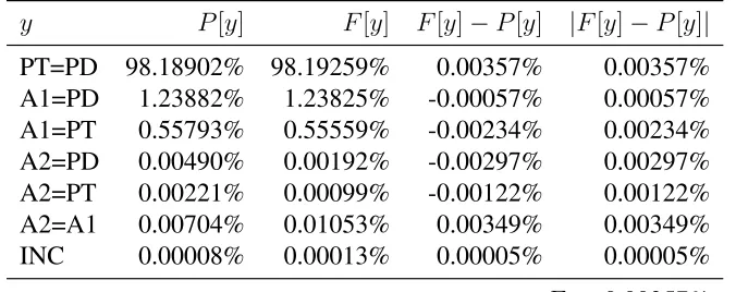
Table 5.1 shows the results obtained for the total sample via the static model. Note that the estimated Truth error rate ET = 0.00357%, which is nearly

160 times as low as the Production Data error rate (EPD = 0.56724%).

Clearly, the Truth is more than precise enough for the purpose of assessing the Production Data Capture system’s data quality. While more than 98% of the fields bypassed the Arbitrator (F[PT=PD] = 98.19259%), the measured manual processing rate MT = 33.23876%, most of which is comprised of

reject keying within the Independent Data Capture system. As we examine the results from the Projector model, we will look for potential opportuni-ties to improve PDQ’s efficiency, while maintaining sufficient overall data quality.

5.2

Projector Model

5.2.1 Projected Truth Error Rate: Method 1

(44)

[image:44.612.142.480.345.479.2]

Table 5.1: Results for total sample: Static model.

(a) Sample size.

Form Count 278,639

fT 5,355,398

(b) Inputs.

EPD 0.56724% EPT 1.25083% EA1 0.39523% EA2 0.39523%

(c) Probabilities, volumes, and Truth error rate.

y P[y] F[y] F[y]−P[y] |F[y]−P[y]|

PT=PD 98.18902% 98.19259% 0.00357% 0.00357% A1=PD 1.23882% 1.23825% -0.00057% 0.00057% A1=PT 0.55793% 0.55559% -0.00234% 0.00234% A2=PD 0.00490% 0.00192% -0.00297% 0.00297% A2=PT 0.00221% 0.00099% -0.00122% 0.00122% A2=A1 0.00704% 0.01053% 0.00349% 0.00349% INC 0.00008% 0.00013% 0.00005% 0.00005%

E_T= 0.00357%

σT= 0.00026%

ET+ 1.645σT= 0.00399%

(d) Manual processing

rate.

(45)

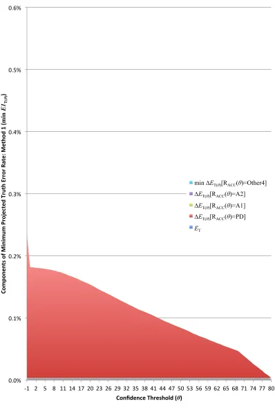
ET(θ), the Truth error rate given by the static model. The largest

er-ror component here is ∆ET(θ)[RACC(θ)=PD]; that is, most of the

Pro-jected Truth errors in this estimate are incurred by newly-accepted fields whose values match incorrect Production Data values. In contrast, the re-maining error components∆ET(θ)[RACC(θ)=A1],∆ET(θ)[RACC(θ)=A2], and min ∆E_T(_θ₎[RACC(θ)=Other4]are negligible.

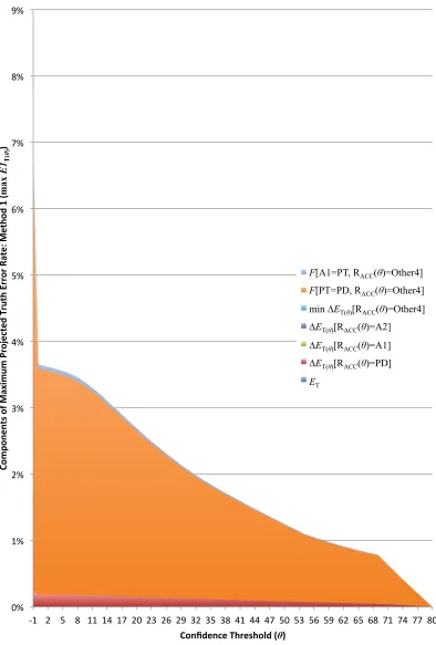
Figure 5.2 shows the components of the maximum estimatemaxE1_T(_θ₎. While there is a noticable contribution from F[A1=PT,RACC(θ)=Other4],

by far the largest error component is F[PT=PD,RACC(θ)=Other4]. As the

confidence threshold decreases, a substantial portion of fields follows the paths (y, z(θ)) = (PT=PD,RACC(θ)=Other4), which yield an indeterminate

projected terminal path y(θ). Assuming that all these fields incur additional Truth errors gives a maximum estimate that increases sharply in contrast to the minimum estimate.

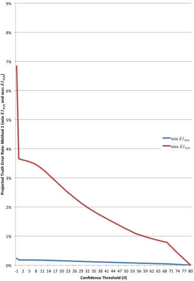
In Figure 5.3 we see a clear comparison of these minimum and maximum estimates.

5.2.2 Projected Provisional Truth Error Rate

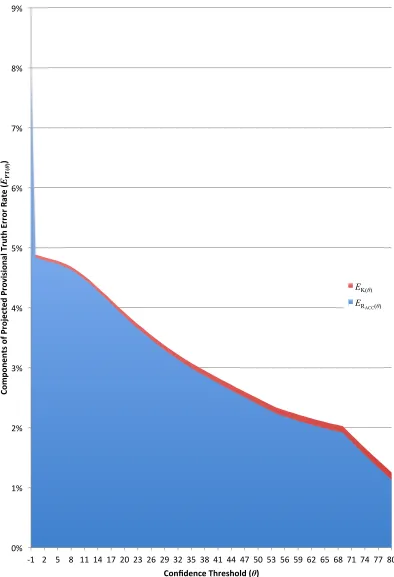
Figure 5.4 shows the components of the projected Provisional Truth error rateEPT(θ), as functions of the confidence thresholdθ. Overall, the projected

error rate increases as the confidence threshold decreases. At all points, the largest error component isERACC(θ), which is contributed by accepted fields. The other error component, EK(θ), consists of projected Keyer errors. This

component starts at less than one tenth of the total at θ = θ0 = 80, and it

decreases slowly as more fields become accepted.

5.2.3 Projected Truth Error Rate: Method 2

Next, we examine the Projected Truth error rates given by Method 2. Figure 5.5 shows the minimum and maximum estimates (minE2T(θ) and maxE2T(θ), respectively), as functions of the confidence threshold θ.

(46)

0.0% 0.1% 0.2% 0.3% 0.4% 0.5%

-‐1 2 5 8 11 14 17 20 23 26 29 32 35 38 41 44 47 50 53 56 59 62 65 68 71 74 77 80

Co

m

po

ne

nt

s

of Mi ni m um P ro je ct ed T ru th E rr or Ra te

: Me

th od 1 ( mi n E1 T( θ ) )

Conﬁdence Threshold (θ)

min ∆ET(θ)[RACC(θ)=Other4] ∆ET(θ)[RACC(θ)=A2]

∆ET(θ)[RACC(θ)=A1] ∆ET(θ)[RACC(θ)=PD] ET

min ∆E_T(_θ₎[R_ACC(θ)=Other4]

∆E_T(_θ₎[R_ACC(θ)=A2]

∆ET(θ)[RACC(θ)=A1]

∆ET(θ)[RACC(θ)=PD]

[image:46.612.109.507.80.671.2]

E_T

(47)

0% 1% 2% 3% 4% 5% 6% 7% 8% 9%

-‐1 2 5 8 11 14 17 20 23 26 29 32 35 38 41 44 47 50 53 56 59 62 65 68 71 74 77 80

Co

m

po

ne

nt

s

of Ma xi m um P ro je ct ed T ru th E rr or Ra te

: Me

th od 1 ( max E1 T( θ ) )

Conﬁdence Threshold (θ)

F[A1=PT, RACC(θ)=Other4] F[PT=PD, RACC(θ)=Other4] min ∆ET(θ)[RACC(θ)=Other4] ∆ET(θ)[RACC(θ)=A2] ∆ET(θ)[RACC(θ)=A1] ∆ET(θ)[RACC(θ)=PD] ET

F[A1=PT, RACC(θ)=Other4]

F[PT=PD, RACC(θ)=Other4]

[image:47.612.111.505.82.665.2]

min ∆E_T(_θ₎[R_ACC(θ)=Other4] ∆E_T(_θ₎[R_ACC(θ)=A2] ∆E_T(_θ₎[R_ACC(θ)=A1] ∆E_T(_θ₎[R_ACC(θ)=PD] ET

(48)

0% 1% 2% 3% 4% 5% 6% 7% 8%

-‐1 2 5 8 11 14 17 20 23 26 29 32 35 38 41 44 47 50 53 56 59 62 65 68 71 74 77 80

Pr

oj

ec

te

d

Tr

ut

h

Er

ro

r Ra

te

: Me

th od 1 ( m in E1 T( θ )

and

max E1 T( θ ) )

min E1T(θ)

[image:48.612.109.509.84.663.2]

max E1T(θ) min E1T(θ) max E1T(θ)

(49)

0% 1% 2% 3% 4% 5% 6% 7% 8% 9%

-‐1 2 5 8 11 14 17 20 23 26 29 32 35 38 41 44 47 50 53 56 59 62 65 68 71 74 77 80

Co

m

po

ne

nt

s

of P ro je ct ed P ro vi si on al T ru th E rr or Ra te (

EPT(

θ

)

EK(θ)

ERACC(θ)

EK(θ)

[image:49.612.110.504.83.660.2]

ERACC(θ)

(50)

0% 1% 2% 3% 4% 5% 6% 7% 8%

-‐1 2 5 8 11 14 17 20 23 26 29 32 35 38 41 44 47 50 53 56 59 62 65 68 71 74 77 80

Pr

oj

ec

te

d

Tr

ut

h

Er

ro

r Ra

te

: Me

th od 2 ( mi n E2 T( θ ) an

d

max E2 T( θ ) )

min E2T(θ) max E2T(θ)

[image:50.612.109.508.84.661.2]

min E2T(θ) max E2T(θ)

(51)

Figure 5.6 compares the various projected error rate estimates. We see immediately that there is close agreement between the respective minimum and maximum Projected Truth error rates given by Methods 1 and 2. Note that minE1T(θ) and minE2T(θ) are within the same order of magnitude,

and that maxE1T(θ) and maxE2T(θ) are very nearly equal. This evidence

supports the validity of Method 1 and Method 2, and of the static model, upon which Method 2 is based directly.

Curiously, there is an almost constant difference between the Projected Provisional Truth error rate E_PT(_θ₎ and either of the maximum Projected Truth error rates maxE1T(θ) and maxE2T(θ). This relationship suggests

that the maximum estimates reflect truly “worst-case” scenarios, in which the Truth error rate is completely dependent upon the Provisional Truth error rate. We can conclude that these maximum estimates are poorly suited for realistic evaluation of PDQ’s performance.

Henceforth, I will use minE2T(θ) as the preferred estimate for practical

purposes.

5.2.4 Projected Manual Processing Rate

We turn now to the estimates of projected manual processing rate given by the Projector model. Figure 5.7 shows the various components of the minimum estimate minMT(θ), as functions of the confidence threshold θ.

Overall, the projected manual processing rate decreases with the confidence threshold. The largest manual processing component is the reject rate FK(θ)

at θ = θ0 = 80, while a greater proportion shifts toward Analyst 1 (FA1) at

lower thresholds. The remaining component, minFA2, is negligible. Note

that unlike the reject rate, the overall minimum projected manual processing rate has a non-zero lower bound (minM_T(₋₁₎ = 8.16987%).

Figure 5.8 shows the components of the maximum projected manual processing rate maxMT(θ). The additional component

F[PT=PD,RACC(θ)=Other4] contributes a significant portion of the overall

manual processing as the confidence threshold decreases. In this estimate, all fields that follow the paths (y, z(θ)) = (PT=PD,RACC(θ)=Other4),

(52)

0% 1% 2% 3% 4% 5% 6% 7% 8%

-‐1 2 5 8 11 14 17 20 23 26 29 32 35 38 41 44 47 50 53 56 59 62 65 68 71 74 77 80

Pr

oj

ec

te

d

Er

ro

r Ra

te

(

Ex

)

Conﬁdence Threshold (θ)

min E1T(θ) max E1T(θ) EPT(θ) min E2T(θ) max E2T(θ) min E1T(θ)

max E1T(θ)

EPT(θ)

min E2_T(_θ₎

[image:52.612.112.511.77.672.2]

max E2_T(_θ₎

(53)

-‐1 2 5 8 11 14 17 20 23 26 29 32 35 38 41 44 47 50 53 56 59 62 65 68 71 74 77 80 0% 4% 8% 12% 16% 20% 24% 28% 32% 36%

Co

m

po

ne

nt

s

of Mi ni m um P ro je ct ed Ma nu al P ro ce ss in

g

Ra te ( mi n MT( θ ) )

min FA2(θ)

FA1(θ)

FK(θ)

min F_A2(_θ₎ F_A1(_θ₎

[image:53.612.105.506.86.637.2]

F_K(_θ₎

(54)

Figure 5.9 shows a clear comparison of minMT(θ) and maxMT(θ). In

contrast to the relationships betweenminE1T(θ)andmaxE1T(θ)or between minE2T(θ) andmaxE2T(θ), the minimum and maximum projected manual

processing rates are within the same order of magnitude at allθ values. In further analysis and discussion, I will use maxM_T(_θ₎ as the preferred, conservative estimate for practical purposes.

5.3

Error and Manual Processing Tradeoff

In Figure 5.10, we see a classic error (EPT(θ)) v. reject (FK(θ)) curve for

the Independent Data Capture system, showing a characteristic tradeoff be-tween the two metrics.

Figure 5.11 shows an analogous relationship between Truth er-ror (minE2_T(_θ₎) and manual processing (maxM_T(_θ₎). The exception, as noted before, is that the manual processing rate reaches a non-zero mini-mum.

While the two visualizations serve equivalent roles for the Independent Data Capture system and for PDQ as a whole, there does not appear to be a simple means to relate one to the other. Figure 5.12 shows an attempt to compare the two curves by setting their respective vertical scales to similar proportions. This demonstrates that it is insufficient to rely on the perfor-mance characteristics of the Independent Data Capture system for tuning operating parameters such as the confidence threshold. To achieve success-ful outcomes, it is essential to understand the relationship between the over-all performance characteristics of PDQ.

5.4

Practical Tuning Application

(55)

-‐1 2 5 8 11 14 17 20 23 26 29 32 35 38 41 44 47 50 53 56 59 62 65 68 71 74 77 80 0% 4% 8% 12% 16% 20% 24% 28% 32% 36%

Conﬁdence Threshold (θ)

Co

m

po

ne

nt

s

of Ma xi m um P ro je ct ed Ma nu al P ro ce ss in

g

Ra te ( max MT( θ ) )

F[PT=PD, RACC(θ)=Other4] min FA2(θ)

FA1(θ) FK(θ)

F[PT=PD, R_ACC(θ)=Other4]

min F_A2(_θ₎

[image:55.612.106.506.85.641.2]

FA1(θ) FK(θ)

(56)

-‐1 2 5 8 11 14 17 20 23 26 29 32 35 38 41 44 47 50 53 56 59 62 65 68 71 74 77 80 0% 4% 8% 12% 16% 20% 24% 28% 32%

Pr

oj

ec

te

d

Ma

nu

al

P

ro

ce

ss

in

g

Ra

te

(

mi

n

MT(

θ

)

an

d

max

MT(

θ

)

min MT(θ)

[image:56.612.103.505.82.677.2]

max MT(θ) min M_T(_θ₎ max MT(θ)

(57)

0% 1% 2% 3% 4% 5% 6% 7% 8% 9%

0% 4% 8% 12% 16% 20% 24% 28% 32% 36%

Pr

oj

ec

te

d

Pr

ov

is

io

na

l T

ru

th

E

rr

or

Ra

te

(

EPT(

θ

)

[image:57.612.114.504.84.659.2]

Projected Reject Rate (F_K(_θ₎)

Figure 5.10: Results for total sample: Projected Provisional Truth error rate (EPT(θ)) v.

(58)

0.0% 0.1% 0.2% 0.3% 0.4% 0.5%

0% 4% 8% 12% 16% 20% 24% 28% 32% 36%

Mi

ni

m

um

P

ro

je

ct

ed

T

ru

th

E

rr

or

Ra

te

: Me

th

od

2

(

mi

n

E2

T(

θ

)

[image:58.612.110.506.85.657.2]

Maximum Projected Manual Processing Rate (max M_T(θ))

(59)

0.0% 0.2% 0.4% 0.6%

0% 3% 6% 9%

0% 4% 8% 12% 16% 20% 24% 28% 32% 36%

Mi ni m um P ro je ct ed T ru th E rr or Ra te

: Me

th od 2 ( mi n E2 T( θ ) ) Pr oj ec te

d

Pr

ov

is

io

na

l T

ru th E rr or Ra te ( EP T( θ ) )

Projected Reject Rate (FK(θ))

Maximum Projected Manual Processing Rate (max MT(θ))

EPT(θ) v. FK(θ)

min E2T(θ) v. max MT(θ)

E_PT(θ) v. F_K(θ)

[image:59.612.110.508.83.649.2]

min E2T(θ) v. max MT(θ)

Figure 5.12: Results for total sample: Comparison of Projected Provisional Truth er-ror rate (EPT(θ)) v. projected reject rate (FK(θ)) and minimum Projected Truth error rate:

(60)

E_PDref = (80%)(1%) + (20%)(3%)

E_PDref = 1.4% (5.1)

While the stated requirements applied strictly to the set of all write-in fields on all forms, we can apply them to the sample at hand for the purposes of evaluating PDQ performance. Let us say that as a rule of thumb, the reference Truth error rate E_Tref should be a tenth of the reference Production Data error rate, and further, that the reference standard error σref_T should be a tenth of the reference Truth error rate. We set our tuning parameters as follows:

D= 10 (5.2)

E_Tref = 0.14% (5.3)

d= 10 (5.4)

σ_Tref = 0.014% (5.5)

Given these parameter values, we can calculate the reference sample size

f_Tref using Equation 3.82 as follows:

f_Tref = (10)(10) 2

1.4% −(10)

2

f_Tref = 71,329 (5.6)

Additionally, we would like to have 95% confidence that our estimated Truth error rate is at or below the reference Truth error rate:

c= 95% (5.7)

zc= 1.645 (5.8)

(61)

was lower than the reference Truth error rate (E_Tref = 0.14%). Thus the conditions for tuning with the Projector model were satisfied.

The tuning chart in Figure 5.13 shows the relationships between the ref-erence Truth error rateE_Tref, Projected Truth error rateminE2_T(_θ₎, and pro-jected manual processing rate M_T(_θ₎, as functions of the confidence thresh-oldθas of Week 3 of May 2010. We wish to find the smallest threshold such that the Projected Truth error rate remains at or below the reference rate.

The critical values for tuning are shown in Table 5.3. A decision might have been made at that time to change the confidence threshold to 44. This would have increased the Truth error rate by a factor of 18 while keeping it below the reference rate. According to the model’s predictions, the same decision would have decreased the manual processing rate to just over half the actual observed rate. At that point in time, PDQ had processed only about 2% of the total selected sample, so the future efficiency improvement would have been quite substantial.

For comparison, Figure 5.14 shows the tuning chart for the total sample as of the end of 2010 Census operations.

Table 5.4 shows some critical values. With the benefit of hindsight, we see that an earlier decision to set θ0 = 44 ultimately would have caused the

Truth error rate (minE2T(θ)+zcσT(θ) = 0.20012%) to exceed the reference

rate. In this case, we see that the “correct” tuning decision would have been to set the confidence threshold to 58, which would have decreased the manual processing rate to about 0.6 times the actual observed rate. A simple solution to this problem would be to continue monitoring a current subsample, approximately equal to the reference sample size, and to trigger a reset to the default, conservative confidence threshold (θ0 = 80) upon

(62)

(a) Sample size.

Form Count 5,057

fT 110,623

(b) Inputs.

EPD 0.49447% EPT 1.05584% EA1 0.58845% EA2 0.58845%

(c) Probabilities, volumes, and Truth error rate.

y P[y] F[y] F[y]−P[y] |F[y]−P[y]|

PT=PD 98.45491% 98.45692% 0.00201% 0.00201% A1=PD 1.04444% 1.04680% 0.00236% 0.00236% A1=PT 0.48637% 0.48724% 0.00087% 0.00087% A2=PD 0.00615% 0.00181% -0.00434% 0.00434% A2=PT 0.00286% 0.00000% -0.00286% 0.00286% A2=A1 0.00516% 0.00723% 0.00207% 0.00207% INC 0.00011% 0.00000% -0.00011% 0.00011%

E_T= 0.00434%

σT= 0.00198%

ET+ 1.645σT= 0.00760%

(d) Manual processing

rate.

[image:62.612.143.480.292.425.2]

FK 31.64532% FA1 1.54308% FA2 0.00904% MT 33.19744%

Table 5.3: Results through Week 3 of May 2010: Tuning values.

θ E_Tref minE2T(θ)+zcσT(θ) maxMT(θ)

[image:62.612.184.430.639.696.2]

(63)

0% 6% 12% 18% 24% 30% 36%

0.0% 0.1% 0.2% 0.3% 0.4% 0.5% 0.6%

-‐1 2 5 8 11 14 17 20 23 26 29 32 35 38 41 44 47 50 53 56 59 62 65 68 71 74 77 80

Ma xi m um P ro je ct ed Ma nu al P ro ce ss in

g

Ra te ( max MT( θ ) ) Mi ni m um P ro je ct ed T ru th E rr or Ra te

: Me

th od 2 ( mi n E2 T( θ ) ) Re fe re nc

e

Tr

ut

h

Er

ro

r Ra

te

(

E

ref T

)

Conﬁdence Threshold (θ)

min E2T(θ)

ErefT max MT(θ)

min E2T(θ)

Eref

T

[image:63.612.112.507.86.670.2]

max M_T(_θ₎

(64)

0% 6% 12% 18% 24% 30%

0.0% 0.1% 0.2% 0.3% 0.4% 0.5%

-‐1 2 5 8 11 14 17 20 23 26 29 32 35 38 41 44 47 50 53 56 59 62 65

Balancing truth error and manual processing in the PDQ system