Detecting glaucoma in biomedical data using image processing

Rochester Institute of Technology

RIT Scholar Works

Theses Thesis/Dissertation Collections

6-30-2005

Detecting glaucoma in biomedical data using image

processing

Mittal Bhatt

Follow this and additional works at:http://scholarworks.rit.edu/theses

This Thesis is brought to you for free and open access by the Thesis/Dissertation Collections at RIT Scholar Works. It has been accepted for inclusion in Theses by an authorized administrator of RIT Scholar Works. For more information, please [email protected].

Recommended Citation

Detecting Glaucoma in biomedical data using image processing

By

Mittal Gopalbhai Bhatt A Graduate Thesis Submitted

in

Partial Fulfillment of the

Requirements for the Degree of MASTER of SCIENCE

in

Electrical Engineering Approved by:

PROF._____________________________ Graduate Thesis Advisor – Dr. Navalgund Rao

PROF._____________________________

Graduate Thesis Committee member – Dr. Maria Helguera PROF._____________________________

Graduate Thesis Committee member – Dr. Raghuveer Rao PROF.______________________________

Electrical Engineering Dept. Head – Dr. Robert J. Bowman

Department of Electrical Engineering COLLEGE OF ENGINEERING

ROCHESTER INSTITUTE OF TECHNOLOGY ROCHESTER, NEW YORK

Thesis Author Permission Statement

Title of thesis: Detecting Glaucoma in biomedical data using image processing Name of author: Mittal Gopalbhai Bhatt

Degree: Master of Science Program: Electrical Engineering

College: Kate Gleason College of Engineering

I understand that I must submit a print copy of my graduate thesis to the RIT Archives, per current RIT guidelines for the completion of my degree. I hereby grant to the Rochester Institute of Technology and its agents the non-exclusive license to archive and make accessible my thesis in whole or in part in all forms of media in perpetuity. I retain all other ownership rights to the copyright of the thesis. I also retain the right to use in future works (such as articles or books) all or part of this thesis.

Print Reproduction Permission Granted:

I, __________________________________, hereby grant permission to the Rochester Institute of Technology to reproduce my print thesis in whole or in part. Any

reproduction will not be for commercial use or profit.

Abstract

This thesis addresses the problem of the early detection of an eye blinding disease, glaucoma. It presents new approaches for analysis of the biomedical scan data of Retinal Nerve Fiber Layer (RNFL) thickness obtained through Scanning Laser Polarimetry that can lead to better tools for early diagnoses of glaucoma. The thickness maps of the RNFL obtained from a Scanning Laser Polarimeter (Gdx-VCC) were used to draw features as opposed to the circular ring one-dimensional data (TSNIT graph) in previous approaches. Fourier analysis and wavelet analysis were performed on the 900

Acknowledgement:

Table of Contents

List of figures and tables……….6

I.

Introduction………....8

II. Glaucoma………...14

III. Retinal nerve fiber layer and Scanning Laser Polarimetry……….19

IV. Analysis of Scanning Laser Polarimetry Image………31

V.

Feature optimization and classification………..41

VI. Experimental results and discussions……….46

VII. Conclusion……….56

References………59

List of Figures and Tables:

Figure 1.1: Photograph of a Scanning Laser Polarimetry Device (Courtesy: Laser Diagnostics, San Diego, CA)

Figure 2.1: Anatomy of the eye (Courtesy: Handbook of Glaucoma (Azuara-Blanco Augusto)

Figure 2.2: Photograph of the optic nerve with optic disc in the center and the areas around it divided into the four sectors – Temporal, Superior, Nasal, and Inferior

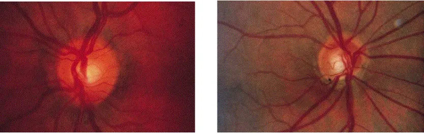
Figure 3.1 Example of optic disc photography

a) normal disc

b) notching in optic disc

(Courtesy: Handbook of Glaucoma (Azuara-Blanco Augusto)

Figure 3.2 Scanning Laser Polarimetry Device – Principle (Courtesy: Laser Diagnostics, San Diego, CA)

Figure 3.3:Color Coded RNFL thickness map of the 65356 points obtained by the SLP (with the color scale on the right).

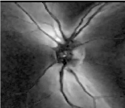
Figure 3.4: Grayscale representation of the RNFL thickness map image.

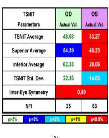
Figure 3.5 a) GDx VCC Printout

b) Parameters with their probability of normality (colorcoded) (Courtesy: Laser Diagnostics, San Diego, CA)

Figure 3.6: Circled region indicates the region to obtain TSNIT graph.

Figure 3.7 a: Nerve fiber layer thickness double-hump patter for non-glaucomatous eye.

Figure 3.7 b: Nerve fiber loss in the superior region resulting in an uneven double-hump patter for a glaucoma patient.

Figure 4.1: Observed butterfly pattern in the 128X256 pixel thickness map of a:

a) Glaucoma scan.

b) Normal eye scan.

Figure 4.2: 90o projections of:

Figure 4.3: Wavelet analysis of the Vertical profile of a Normal scan (only second level detail coefficients shown).

Figure 4.4: Wavelet analysis of the Vertical profile of a Glaucoma scan (only second level detail coefficients shown).

Figure 4.5: Two Dimensional Fourier Transform of: a) “Glaucomatous” scans.

b) “Normal” scans.

Figure 4.6: Average image of:

a) “Glaucomatous” scans. b) “Normal” scans.

Figure 4.7: Pattern image derived from Normal average scans: a)Left eye.

b) Right eye.

Figure 6.1: ROC curve for Fourier analysis of 90o _projection.

Figure 6.2: ROC curve for Wavelet - Fourier analysis of 90o projection.

Figure 6.3: ROC curve for 2D Fourier analysis.

Figure 6.4: ROC curve for Correlation coefficient.

Figure 6.5: ROC curve for Combined Feature set.

Figure 6.6: ROC curve for FT of TSNIT graph.

Figure 6.7: ROC curves for (red) Combination of all current features (blue) FT of TSNIT graph.

Chapter 1

Introduction

consisting of medication or surgery to reduce the intraocular pressure. Hence the diagnosis of glaucoma at an earlier stage is very important for its treatment.

A major concern with glaucoma detection is that the disease has no particular set of physical causes or symptoms that doctors can recognize to detect the disease in an early stage.4 The main focus in glaucoma diagnosis is to detect changes in the visual functioning of the eye at early stages of the disease so that vision can be protected and preserved through medical treatment. It has been proved that the development of visual field defects is preceded by RNFL damage in glaucoma.5 Studies show that as much as 40% of retinal nerve fiber in the eye can be lost without the detection of characteristic visual defect in glaucoma patients.6 Hence it is believed that the detection of damage in nerve fiber layer can lead to an early detection of glaucoma. Several computer-assisted imaging technologies for detecting the structural changes in the retinal nerve fiber layer have been developed. The assessment of the ganglion cell structure is based on measuring the thickness of the retinal nerve fiber layer.

measurable phase shift of polarized laser beam double passing the RNFL. This is found to be proportional to the thickness of the nerve fiber layer.8, 9 This retardation (degrees) information is converted to thickness (microns) through the conversion factor based on the histologic comparison with monkey eyes.10 A new version of the device (GDx-VCC) is designed to individually compensate for the effects of birefringent properties of other parts of the eye like the cornea. The device provides a large array of points corresponding to retinal never fiber layer thickness at each respective point across the back of the eye. The scans thus available are in the form of 128 X 256 images or gray-level thickness maps. The goal of this thesis is to analyze these scans and develop classification techniques for them.

Figure 1.1 Photograph of a Scanning Laser Polarimetry Device (Courtesy: Laser Diagnostics, San Diego, CA)

and reliable set of features is to make them statistically independent. A very effective way to achieve this end is to perform Principal component analysis on the feature set11. This will help in reducing feature dimension by eliminating redundancy caused by interdependencies in the feature vector. The last step is the classification of the data set into the two classes. Fisher’s Linear Discriminant Analysis (LDF) provides an easy and robust way of linearly classifying different classes by projecting the feature vector so that it maximizes class separability12.

Previous Work:

The Scanning laser polarimetry devices provide a number of software-generated parameters, the main ones being the software generated parameters as ‘the number’ and the ‘NFI’ (nerve fiber indicator). Reports have shown that GDx software generated parameters have limited ability for glaucoma detection.13-23 Several other approaches for the analysis of the scan data available through these devices have been presented to improve upon these results. Locally based techniques like relative surface height,17 and sectoral-based analysis18 _{have been reported with better results than GDx parameters.}

One approach proposed a linear discriminant function combining GDx parameters and found better result than the ‘number’.16 Another approach proposed discriminant analysis of 300 sectoral data from the scanning laser polarimetry.19 A lot of proposed techniques use the data obtained from a circular ring band around the center of the optic disc in the scan data. The inner radius of the ring is taken to be 1.75 times the disc diameter.20 _A

different techniques. In some more robust approaches the global shape analysis of the double hump curve has been suggested and found to better in identifying glaucomatous patients. These techniques include Fourier analysis suggested with different number of sampling as well as different combinations of the Fourier analysis components.19-22 Wavelet-Fourier analysis of the one-dimensional data has also been proposed and shown to have better identification power as compared with the ‘number’.23

The techniques used currently for the analysis of the scan data from the Scanning laser polarimetry devices have chiefly depended on the ring data around the optic disc center. The scan is divided into four sectors known as the Temporal, Superior, Nasal, and Inferior and hence the data obtained from the ring around the optic disc is called the TSNIT graph. Although these data provide considerable amount of information for glaucoma recognition, the information in the rest of the scanned image must not be completely neglected. In order to further improve the performance of the classifier, Fourier analysis of the data obtained using the entire region of the scan as well as analysis of the two dimensional Fourier transform of the scan is proposed.

Chapter 2

Glaucoma

The term ‘glaucoma’ refers to a large number of optic nerve diseases, which is associated with loss of visual activity and can lead to total, irreversible blindness if left untreated24_{. Glaucomatous optic neuropathy is the second leading cause of blindness}

worldwide.

These axons originating in the ganglion cell layer of the retina, the innermost layer of the eye, form the retinal nerve fiber layer (RNFL). These axons collect the visual information and carry it outside the eye via the optic nerve. The nerve head is the distal portion of the optic nerve. The retinal nerves converge upon the nerve head from all points of the fundus. The portion of the optic nerve head that is clinically visible by an ophthalmoscope is known as the optic disc. The optic nerve head is slightly vertically oval and it is also the site of entry for the retinal vessels. The shape and size of the optic disc is important in evaluation for glaucoma diagnosis.

Figure 2.1 Anatomy of the eye

(Courtesy: Handbook of Glaucoma (Azuara-Blanco Augusto)

glaucomatous damage) is usually defined as 15.5 +_ 2.5 mmHg while ‘glaucomatous’ IOP is generally described as above 20.5 mmHg. However, glaucoma patients are known to have IOP within the normal range and raised IOP can be found in non-glaucomatous eyes. Intraocular pressure is subject to a certain daily variation as well as variation during the same day24. Normal eyes show less diurnal variation in the IOP than glaucomatous eyes. The elevated IOP when beyond that compatible with normal ocular function leads to irreversible damage to the nerve fibers in the retina, thus causing visual impairment. Intraocular pressure has a central role in the treatment of all forms of glaucoma today. It has been considered the main risk factor for glaucoma, and almost every treatment for glaucoma patient is aimed at reducing the IOP. Although raised IOP is considered a big risk factor for glaucoma, alone it is insufficient for the diagnosis of most forms of glaucoma. It has been associated with only 50% sensitivity and 90% specificity.6 However it still is the primary criterion for making diagnosis for patients with normal optic nerve heads and normal visual fields as well as in cases of congenital and secondary glaucoma. The most widely used and accepted gold standard for measuring IOP is Goldmann tonometry. Goldmann determined that when an area of 3.06 mm in a human eye is flattened with 520 µm corneal thickness, then resistance of cornea balances with the surface tension and hence could be ignored. This is the main principle on which the tonometer is based.

a very important characteristic to determine glaucomatous damage. The shape of the optic disc in a normal eye is round or horizontally oval. The region in the retina around the optic disc has been divided into four areas, the horizontal sector towards the nose is called the Nasal region, the other horizontal sector being the Temporal, the vertical sector above the disc is known as Superior while the sector below is called Inferior (Figure 2.2). The neural rim around the optic disc is widest in the inferior quadrant, followed by superior, nasal and temporal.

There are various patterns of optic disc changes in glaucoma, and the detection of change is the diagnosis of glaucoma. The concentric enlargement of the optic cup, notching, and other similar patterns of glaucomatous damage are the most commonly found. The optic disc to optic cup ratio is therefore usually taken into consideration while evaluation. However the asymmetries of cup/disc can have other diseases as a cause and are therefore not as reliable. Other features taken into account are the size and shape of

Figure 2.2 Photograph of the optic nerve with optic disc in the center and the areas around it divided into the four sectors – Temporal, Superior, Nasal, and Inferior.

direct examination of the optic disc through an ophthalmoscope is called ophthalmoscopy and it can provide useful information for diagnosis of glaucoma. It is generally performed in a dark room with dilated pupil. Although doctors can detect a lot of features through this technique, it does not yield a permanent record and has interobserver and intraobserver variabilities. Its sensitivity and specificity has been reported to be only 59% and 73%, respectively.7

A careful examination and detection of change in the optic nerve and the nerve fiber layer is the key to early diagnosis of glaucoma. There are several instruments currently available for imaging of optic nerve and the nerve fiber layer, such as red-free photography, the Topcon ImageNet system, the confocal scanning laser ophthalmoscope, the retinal nerve fiber layer analyzer, and the optical coherence tomograph. The main disadvantages of these techniques however, are the lack of adequate amount of research and high cost.

Chapter 3

Retinal Nerve Fiber Layer and

Scanning Laser Polarimetry

while the central axons take a more superficial path and follow the innermost part within the optic nerve head. Due to the characteristic pattern of the nerve fiber layer axons, the thickness of the nerve fiber layer on the vertical poles of the optic disc is much higher than in the nasal and temporal optic disc poles. The importance of the detection of RNFL damage as an early sign of glaucoma has been confirmed by numerous studies. Hoyt and Newman first described it in 198725,26. Histological studies show that as much as 40% of retinal nerve fiber in the eye can be lost without the detection of characteristic visual defect in glaucoma patients6_{. The findings of Sommer and colleagues showed that RNFL}

damage could precede visual field loss by up to 5 years27. Hence it is believed that the detection of damage in nerve fiber layer can lead to an early detection of glaucoma.

RNFL defects related to glaucoma can be either diffused or localized. Localized defects generally include slit-like or groove-like defects in the RNFL. When these slit like defects extend to the disc margin or the wedge shaped defects are seen as notches in the neuroretinal rim in inferior or superior regions, it is judged as a sign of glaucomatous abnormality. Although localized defects are easier to detect, diffuse RNFL loss is more common and difficult to diagnose. The second order retinal vessels, which are normally well concealed by the retinal nerve fiber layer, start to be seen in this kind of defects. The progressive loss of RNFL thickness in the superior and inferior poles is a sign of glaucomatous damage.

techniques include examination of the retina through a dilated pupil using an ophthalmoscope or by using a red-free camera or using high-resolution black and white photographs. These are all, however, limited by the pupil size and media optics and tend to have high intra- and interobserver variability. To reduce these difficulties and provide more quantitative measurements of the nerve fiber layer, different devices have been developed. Several instruments have been developed that focus on imaging of the fundus (a mirror like structure just behind the retina which acts as a light amplifier) and analyzing the topography of the retinal surface28,6,7_{. These methods attempt to quantify}

Figure 3.1 Example of optic disc photography a) normal disc b) notching in optic disc (Courtesy: Handbook of Glaucoma (Azuara-Blanco Augusto)

thickness of the RNFL due to its properties and it can be measured using a polarimeter. This retardation (degrees) information is converted to thickness (microns) through the conversion factor based on the histological comparison with monkey eyes.10

Figure 3.2 Scanning Laser Polarimetry Device - Principle (Courtesy: Laser Diagnostics, San Diego, CA)

The Scanning Laser Polarimeter uses this principle to scan the thickness of the retinal nerve fiber by employing a low power near infrared laser beam to illuminate the human retina. The device using this technology is currently available through Laser Diagnostic Technologies, Inc, San Diego, CA. The device scans the retina with laser beam and measures the retardation at 65,536 discrete points within the retinal area of 15o by 15o in less than 1 second. The software application displays this retardation information on a computer screen as a color-mapped image of the retina (Figure 3.3). A grayscale image of the thickness map of the same retina is also showed in figure 3.4 for reference. The software also provides other software generated information and parameters extracted from the thickness map. The company has generated a normative

Retardati

Ligh

t

Polariz

er

Two polarized

components

Birefringent

structure

database using the thickness maps obtained from variety of patients as well as normal eyes. This is then used to compare the parameters obtained from current patient to provide the probability of the patient having glaucoma based on those parameters. These computer generated parameters include summary measures based on the calculation circle (Figure 3.5).

Figure 3.3 Color Coded RNFL thickness map of the 65356 points obtained by the SLP (with the color scale on the right).

Figure 3.4 Grayscale representation of the RNFL thickness map image

the disease on subjective basis. Reports have shown that GDx software generated parameters have limited ability for glaucoma detection.18-23 One analysis approach proposed a linear discriminant function combining GDx parameters and found better result than the ‘number’14. Several different analyses of the data have been approached and will be discussed briefly.

(a)

Norma

l

Glaucom

a

Fundus Image

Paramete rs

Thickness Map

Deviation Map

(b)

Figure 3.5a) GDx VCC Printout b) Parameters with their probability of normality (colorcoded) (Courtesy: Laser Diagnostics, San Diego, CA)

To assess the condition of the nerve fiber layer for more analysis, data is extracted from the thickness map by placing a circle at a specified distance around the optic nerve head. The scan image provided by the SLP is divided into four sectors defined as temporal (335o-24o), superior (25o-144o), nasal (145o-214o) and inferior (215o-334o). As shown in figure 3.6, the data from the circled region is taken and plotted to analyze the RNFL thickness. Going from 0o _{around the circle in the 10-pixel band, the circle is}

divided into 16, 32 or 64 sectors, and for each sector the thickness values in the band are averaged and taken as a corresponding point value for the graph. This results into the TSNIT graphs shown in figure 3.6. The RNFL around the optic nerve head show a thicker distribution in the superior and inferior regions in a normal eye according to histopathological measurements30_{. When the thickness of the nerve fiber layer around the}

Figure 3.6 Circled region indicates the region to obtain TSNIT graph

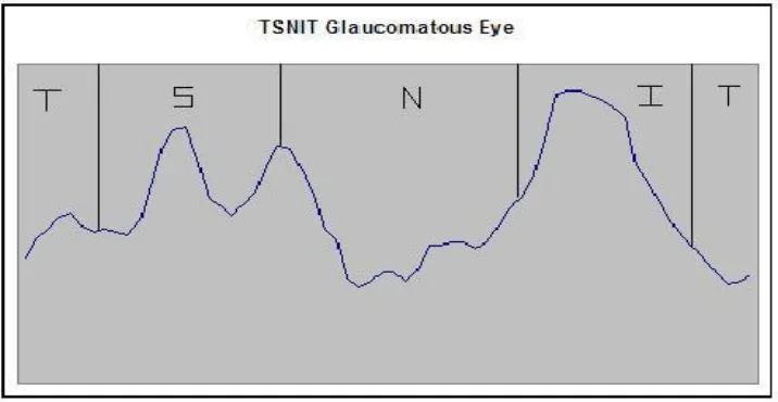
The double hump pattern found more commonly in non-glaucomatous eyes has humps or high value peaks in the superior and the inferior regions and very low thickness values in the temporal and nasal regions. This can be observed in the graph shown in figure 3.7 which has been obtained from the SLP scan of a non-glaucomatous eye. This double hump pattern is expected to be generally present for eyes without glaucomatous damage since the thickness of the nerve fiber layer has been observed to be higher in superior and inferior regions according to histological studies. Glaucoma leads to loss of nerve fiber layer either in all regions or comparatively more damage in the superior and inferior regions. In the first case the whole TSNIT graph has a general decrease in height or thickness intensity whereas in the other case either higher loss is found in superior or inferior region of the retinal nerve fiber layer or both. Figure 3.7b shows the graph for a glaucomatous eye with more loss in the superior sector as compared to other regions.

10 pixels 20

30 pixels T

S

N

Figure 3.7a Nerve fiber layer thickness double-hump patter for non-glaucomatous eye

Figure 3.7b Nerve fiber loss in the superior region resulting in an uneven double-hump patter for a glaucoma patient

the inner radius of the band since it has been observed to be the most stable region with regards to the observed graph pattern. Local measures like the correlations of thickness values in superior and inferior sectors, peak-to-trough amplitude in the two humps as well as mean thickness values have been analyzed as parameters20. Other techniques based on local measures like relative surface height17, and sectoral-based analysis18 have also been reported with better results than GDx parameters. Another approach proposed discriminant analysis of 300 sectoral data from the scanning laser polarimetry16.

Some other techniques are based on a global shape analysis of the double-hump pattern and have proved to be more robust. One approach for the analysis of the double-hump patter is to describe it using Fourier analysis. Several studies have been made using Fourier analysis, using either single Fourier coefficients to differentiate/detect glaucoma or various combinations21, 22_{. The sensitivity and specificity of these methods were}

All these techniques are an improvement in general to the machine generated parameters or the ‘number’ alone. These techniques however use only a part of the two dimensional data obtained from scanning the entire 15o _{area of the retina. Thus around}

75-80% of the data in the SLP scan image is never really used for analysis and detection of the disease. The center of the optic disc and its radius are determined manually by a technician or an observing ophthalmologist and is thus subjective. The data obtained from the circular band, although has been observed to be stable in that region is still subjective to the correct determination of the center and radius of the disc. All these factors lead to a need for more analysis of the image as a whole and to extract features that are derived by using more information rather than limiting it to one part of the image.

Chapter 4

Analysis of Scanning Laser Polarimetry

Image

Diego) was kind enough to share around 10 images of each case along with other analysis information that the SLP machine calculates, from his previous experiments. The company’s latest machine, GDx VCC was used to obtain these scans. VCC stand for Variable Corneal Compensation. Studies show that other regions of the eye, like the cornea and crystalline lens also possess some birefringent properties. Since this will affect the scan data by adding to the RNFL thickness calculation according to the thickness of those structures, this affects the accuracy of the scanned thickness map. An anterior segment compensator assumes a fixed slow axis of corneal birefringence and it aligns its axis with the corneal polarization axis to cancel the effect of corneal birefringence without affecting RNFL polarization31. The GDx VCC is a scanning laser polarimeter, which employs the compensation technique to take care of the birefringent properties of other parts of the ocular region scanned by the laser beam. Thus the GDx VCC was a better choice to obtain the data than the previous devices by the company32,33_.

experiment with these images and to figure out acceptable and useful features that could help improve on the analysis of the scans for detection of glaucoma.

a b

Fig. 4.1 Observed butterfly pattern in the 128X256 pixel thickness map of

a) Glaucoma and b) Normal eye scans

The images used are a general size of 128 X 256. The data of the entire image is used and hence the final classification is not to be affected by the location of the center of the optic disc in the image. It was observed that the retinal scan has a butterfly pattern (Fig.4.1) and hence it gives rise to the double-hump pattern of the TSNIT graphs. Hence various projections of the image were taken assuming that some useful information can be extracted from it. The general idea is to base the obtained one dimensional data on the whole region covered by the retinal nerve fiber layers instead of on the circular band region and at the same time eliminate the necessity to calculate the center or radius of the optic disc. The projections taken were: 0o_{, 90}o_{, 25}o_{, 45}o_{, 145}o _{and 135}o_{. However, as}

a b

Fig. 4.2 90o _{projections of a) “Normal” and b) “Glaucomatous” scan}

Function. Both of these analyses will be discussed in the next chapter along with the results.

Fig. 4.3 Wavelet analysis of the Vertical profile of a Normal scan (only second level detail coefficients shown here)

mother wavelet. If f(t) is a square integrable function, then the discrete wavelet transform (DWT) pair of the function with respect to a wavelet ψ(t)and the scaling function φ(t) is defined as

=

x j k

x x f M k j

Wφ( ₀, ) 1 ( )

ϕ

=

x jk

x x f M k j

Wψ( , ) 1 ( )

ϕ

and

−

−

+

= _{0 ,} 1 _,

0

0 ( , ) ( )

1 ) ( ) , ( 1 ) ( J j

j k jk

k j k

x k j W M x k j W M x

f _φ

ϕ

ψ

Fig. 4.4 Wavelet analysis of the Vertical profile of Glaucoma scan (only second level detail coefficients shown here)

In order to reflect small changes in the signal structure that may be lost by the Fourier analysis, a 2nd _{level wavelet transform was performed using an 8}th_{-order wavelet}

named “Symmlets”, along with the Fourier analysis of the profile. The vertical profile was decomposed using wavelet analysis (M = 128) and the detail coefficients from the second level (32 points) were used and combined with the Fourier transform of the average coefficients after normalizing (to range [0,1]) as a feature set.

a b

The Fourier analysis of the entire scan image provides as well some useful features due to the butterfly pattern from the center of the optic disc. In order to capture the pattern of the entire scan data, the two-dimensional Fourier Transforms (FT) of the images was taken. The 2D Fourier transform of the “normal” scans (Fig. 4.5b) were observed to have several ‘spike’ like streaks coming out in various directions from the center, as opposed to an almost even spread center region in the Fourier transform of the “glaucoma” (Fig. 4.5a) scans. This is believed to be a direct result of the butterfly pattern in the original scans. Hence features can be drawn out to define the spike pattern in the Fourier transform. For this purpose, a circular ring band at an inner radius of 20 pixels and width of 10 pixels band was extracted. 64-point data were obtained from this circular ring band around the center of the two-dimensional Fourier transform. Since the Fourier transform is symmetric only one quarter of the points drawn out from the circular band needs to be used.

a b

Fig 4.7 Pattern image derived from Normal average scans a) Left eye b) Right eye

Chapter 5

Feature Optimization And

Classification

Feature Optimization:

The main objective of this step in the classification process is to reduce the dimension of the feature vector without losing the variability of the feature set. Principal Component analysis (PCA) identifies linear combinations of the feature set so that most of the variability (information) of the original feature set is contained within that combination11,12,37. It essentially transforms a feature vector with correlated variables into a smaller sized feature vector with uncorrelated variables. These uncorrelated variables are called the principal components. The first principal component is the projection of the data points (points in the feature set/ feature vector) in the direction of the line giving the best orthogonal regression fit to the data points. Since the best fit to this type should pass through the mean, the data points are centered on the mean by subtracting the mean from the data points. The first principal component is hence the projection of the data points into the direction with maximal variance of the projected points. The first principal component corresponds to the maximum variability of the original feature set and the second component corresponds to the second highest variability of the set and so forth, there are p principal components (p is the feature vector size).

principal component directions. A matrix A is calculated by using the ordered eigenvectors of the covariance matrix of the feature vectors. The transformation matrix is then extracted from A by taking the eigenvectors corresponding to only the k largest eigenvalues. The new transformation matrix Akis then used to derive the new compressed

feature vector of dimension k.

Classification:

The compressed feature vectors obtained in the last step are now passed through a classification process that decides whether the feature vector belongs to “normal” group or “glaucomatous” group. The classifier predicts the membership of each sample in the data set based on its feature vector. In a linear discriminant analysis (LDF) 11,12,37, a linear combination of the feature vector variables is fed to the classifier to predict group membership. First a trainee set is used where the feature vector and the group membership are known. This is then used to form a model that can be used as the classifier. The Fisher’s LDF has been used as a classifier for its simplicity and robustness.

groups (Sample_Mean). This will generate three different average vectors that are then used to find the between-groups and within-group variability. If the p dimensional sample feature vector sets corresponding to the two classes are described by the xi1and xi2, then

the sample mean vectors are defined by

=

= ni

j ij

i i

n 1

1 _x

x i = 1,2 (1)

and the overall mean vector is defined as

= = = ₂ 1 2 1 i i i i i n n x

x (2)

Thus the overall mean (SampleMean) is taken as the weighted average of the samples since it is weighted by niwhich is the number of samples in the corresponding ith trainee

group set. Next, the between-groups variability matrix B is defined as

T i

i i i

n ( )( )

2 1 x x x x

B= − −

=

(3)

and the within-group variability matrix W is defined as

T ij i i n j ij i i

n 1) ( )( )

( 2 1 2 1 1 x x x x

W= − − −

= = =

(4)

The Fisher’s LDF is based on the idea to find a coefficient vector a that maximizes separation of the samples while making the classification of the groups a linear process.

Hence in order to find a vector a, such that it maximizes

Wa a Ba a T T

, the eigenvalues and

eigenvectors of the matrix W-1_{B are calculated and the eigenvector corresponding to the}

dimensional feature vector obtained from the PCA analysis is converted to a single dimension using the Fisher’s LDF and then using a single threshold (linear discriminant), the sample data can be divided into two separate groups.

Chapter 6

Experimental results & Discussion

analysis for performance evaluation was done and its theory is explained briefly in the next section.

Receiver Operating Characteristic (ROC) curve:

obtained from the company records upon request but is outside the scope of this thesis to be attached as a proof.

classification of any sample has 100% chance of being true. Thus the closer the value of area is to 1, the better classifier performance. In addition to this value, the best values of sensitivity for corresponding specificity are also observed from the ROC curve and noted to show the performance of the classifier.

Classification techniques (using different feature sets) and ROC curves:

Feature Set 1 - Fourier transform of vertical profile of the scans:

multidimensional feature vector into a single dimension while maximizing the group variability. The results of the discriminant analysis showed sensitivity and specificity of 75.12% and 99.15% respectively. The receiver-operating curve (ROC) for this feature is as shown in Fig. 6.1 and the area under the curve is 0.7789.

Feature Set 2:Wavelet analysis of the vertical profile of scans

The next feature vector to be analyzed was the detail coefficients from the second level (32 points) of the wavelet analysis of the vertical profile, combined with the Fourier transform of the approximation coefficients. Since two different sets of values are being combined here, the values of each were normalized to the range of [0,1] before

Figure 6.1 ROC curve for Fourier analysis of 90o _projection

Figure 6.2 ROC curve for Wavelet - Fourier analysis of 90o _projection

Feature Set 3: Ring data from two-dimensional FT of the scans

Figure 6.3 ROC curve for 2D Fourier analysis

Feature Set 4: Ring data from two-dimensional FT of the scans

The fourth feature set simply consisted of a single feature, the correlation coefficient of the scan images with the generated pattern image. The ROC curve for this feature is shown in figure 6.4 and has an area under the curve of 0.8287 with sensitivity and specificity of 67.5% and 82% respectively.

Figure 6.4 ROC curve for Correlation coefficient

thus consisted of the 64 point FT of the projection of the scan data, 32 point second level detail coefficients from the wavelet transform, 32-point ring data from the 2D FT of the scan as well as the correlation coefficient, thus making it a 128-point feature vector. The first 15 principal components were found to contain about 98% of the variability and hence were used for the LDF. The results of the LDF analysis using a uniform and random division of the data set showed comparable results to the existing techniques that are under study for the analysis of the GDx-VCC scans. The ROC curve for the entire feature set is shown in figure 6.5. The area under the curve is 0.8433 with sensitivity and specificity of 84.68% and 91.3% respectively.

Figure 6.5 ROC curve for Combined Feature set

figure 6.6 and its area under the curve was found to be 0.8566 and sensitivity and specificity values of 76.79% and 91.3% respectively.

Figure 6.6 ROC curve for FT of TSNIT graph

Figure 6.7 ROC curves for

A comparison of the ROC curves for both the classification systems can be seen in figure 6.7. Table 6.1 shows the comparisons of the area under the curve, sensitivity and specificity values for all the different feature sets used, the final combination of all the proposed features into one feature set as well as the Fourier analysis of the TSNIT graph.

Table 6.1 Performance evaluation of the different feature sets based on the ROC analysis using the same trainee and test set, chosen randomly and uniformly

Method Sensitivity Specificity Area under ROC curve

FT of 900 _{projection 75.12% 99.15% 0.7789}

Wavelet analysis with

FT of 900 _{projection 58.7% 89%. 0.8235}

Ring data from 2D FT 74.92% 91.5% 0.7813

Correlation coefficient

with pattern image 67.5% 82% 0.8287

Combined Feature set 84.78% 91.3% 0.8433

FFTA – based on previously performed

Chapter 7

Conclusion

vertical projection data is just a horizontal slice of the two-dimensional Fourier transform (2D-FT) of the scan. Therefore the two methods using the Fourier analysis amount to extracting two subsets of information from the 2D-FT. One is a vertical slice of 2D-FT and the other over a ring in the 2D-FT. Both have been seen to be useful for classification. Although the area under the curve obtained for these features was not as good as the other feature sets, the best sensitivity obtained for high specificity showed significant prospect of its use in aiding the classification process. The wavelet analysis in addition to the Fourier analysis of the projection data was found to give a high area under the curve, although failing to produce respective high sensitivity for required specificity. Nevertheless, the feature provides high separability and hence was added to the feature set for the final classification. The pattern image used for correlation coefficient feature has proved to capture most of the pattern found in the normal scans vs. the glaucoma scans and has given comparable results to the previous work by just using the single feature. More pattern images to capture thoroughly the differences in the scan patterns are proposed for future work.

References

1. NT Choplin, DC Lundy, Atlas of Glaucoma, Martin Dunitz Ltd., 1998.

2. The International Bank for Reconstruction and Development/the World Bank: World Development Report 1993. Oxford: Oxford University Press, 1993.

3. HA Quigley, Number of people with glaucoma worldwide’, Br J Ophthalmology, 1996; 80:389–93.

4. J Green, H Siddall, I Murdoch, Learning to live with glaucoma: a qualitative

study of diagnosis and the impact of sight loss, Social Science and Medicine,

2002; 55(2): 257-267

5. A Tuulonen, J Lethola, PJ Airaksinen, Nerve fiber layer defects with normal visual fields. Do normal optic disc and normal visual field indicate absence of

glaucomatous abnormality?, Ophthalmology, 1993; 100:587-98

6. HA Quigley, GR Dunkelberge, WR Green, Retinal ganglion cell atrophy

correlated with automated perimetry in human eyes with glaucoma, Am J

Ophthalmology, 1989; 107:454 – 64

7. AW Dreher, K Reiter, RN Weinreb, Spatially resolved birefringence of the retinal

nerve fiber layer assessed with a retinal laser ellipsometer, Applied Optics, 1992;

31:3730-3735

8. AW Dreher, ED Bailey, Assessment of the retinal nerve fiber layer by

scanning-laser polarimetry, SPIE Ophthalmic Technologies III, 1993; 1877:266-271

9. AW Dreher, K Reiter, Scanning laser polarimetry of the retinal nerve fiber layer, Polarization Analysis and Measurement, 1992; 1746:34-41

10. RN Weinreb, AW Dreher, A Coleman, H Quigley, B Shaw, K Reiter,

Histopathology validation of Fourier-ellipsometry measurements of retinal nerve

fiber layer thickness, Arch Ophthalmology, 1990; 108:557-560

11. RC Gonzalez, RE Woods, Digital Image Processing (second edition), Prentice Hall, 2002

12. S Theodoridis, K Koutrousmbas, Pattern Recognition, Academic Press, 1998 13. Tjon-Fo, MJ Sang, HG Lemij, The sensitivity and specificity of nerve fiber layer

measurements in glaucoma as determined with scanning laser polarimetry, Am J

14. RN Weinreb, L Zangwill, CC Berry, et al., Detection of glaucoma with scanning

laser polarimetry, Arch Ophthalmology, 1999; 117:1298-1304

15. JR Trible, RD Schultz, JC Robinson, et al. Accuracy of scanning laser

polarimetry in the diagnosis of glaucoma, Archives of Ophthalmology, 1993;

117:1298-304

16. C Bowd, LM Zangwill, CC Berry, et al., Detecting early glaucoma by assessment

of retinal nerve fiber layer thickness and visual function, Invest Ophthalmol Vis

Sci, 2001; 42:1993-2003

17. J Caprioli, J Miller, Measurement of relative nerve fiber layer surface height in

glaucoma, Ophthalmology, 1989; 96:633-641

18. FA Medeiros, R Susanna(Jr.), Comparison of algorithms for detection of localized

nerve fiber defects using scanning laser polarimetry, Br J Ophthalmology, 2003;

87:413-419

19. MJ Greaney, DC Hoffman, DF Garway-Heath. et al, Comparison of optic nerve

imaging methods to distinguish normal eyes from those with glaucoma, Invest

Ophthalmol Vis Sci, 2002; 43:140-5

20. MJ Sinai, EA Essock, RD Fechtner, N Srinivasan, Diffuse and Localized nerve fiber layer loss measured with a scanning laser polarimeter: sensitivity and

specificity of detecting glaucoma, J Glaucoma, 2000; 9:154-162

21. EA Essock, MJ Sinai, RD Fechtner, N Srinivasan, FD Bryant, Fourier Analysis of nerve fiber layer measurements from scanning laser polarimetry in glaucoma:

emphasizing shape characteristics of the ‘double-hump’ pattern, J Glaucoma,

2000; 9:444-452

22. EA Essock, MJ Sinai, LM Zangwill, RN Weinreb, Fourier analysis of OCT and

GDx RNFL measurements in diagnosis of glaucoma, Arch Opthalmology, 2001;

23. Y Zheng, EA Essock, A novel feature extraction method- wavelet-Fourier

analysis and its application to glaucoma classification, conference paper, 5th

CVPRIP, 2003

24. AB Augusto, Handbook of Glaucoma, London, UK, Taylor, 2001

25. WF Hoyt, LL Frisén, NM Newman. Funduscopy of nerve fiber layer defects in

glaucoma. Invest Ophthalmol 1973; 12:814-829[Medline].

26. WF Hoyt, B Schlicke, RJ Eckelhoff. Funduscopic appearance of a nerve fiber

27. A Sommer, J Katz, HA Quigley et al. Clinically detectable nerve fiber atrophy

precedes the onset of glaucomatous field loss. Arch Ophthalmol 1991; 109:77-83

28. RH Webb, GW Hughes and FC Delori. Confocal scanning laser ophthalmoscope. Appl. Opt. 1987; 36:1492-1499

29. O Wiener, Die Theorie des Mischikorpers fur das Feld der Stationaren Stromung, Abh. Sachs. Ges. Akad. Wiss. Math. Phys. KI. 1912; 32:507-604

30. TE Ogden, Nerve fiber layer of the primate retina: Morphological analysis. Invest. Ophthalmol. Vis. Sci. 1984; 25:19

31. DS Greenfield, RW Knighton, X Huang, Effect of corneal polarizationaxis on

assessment of retinal nerve fiber layer thickness by scanning laser polarimetry.

Am. J Ophthalmol. 2000; 129:715-722

32. Q Whou, RN Weinreb, Individualized compensation of anterior segment

birefringence during scanning laser polarimetry. Invest Ophthalmol. 2002;

43:2221-2228

33. RN Weinreb, C Bowd, LN Zangwill. Glaucoma detection using scanning laser

polarimetry with variable corneal compensation. Arch Ophthalmol. 2003;

121:218-224

34. RM Rao, AS Bopardikar, Wavelet Transforms: Introduction to Theory and

Applications. Pearson Education (Singapore), 1998

35. O Rioul, M Vetterli, “Wavelets and signal processing”, IEEE Signal Processing Magazine, October 1991; 14-38

36. SG Mallat, “A theory for multiresolution signal decomposition: The Wavelet

Representation”, IEEE Transactions on Pattern Analysis and Machine

Intelligence, 1989; Vol II, 7:674-693

37. GJ McLachlan, Discriminant Analysis and Statistical Pattern Recognition, Wiley, New York, 1992

38. DM Green, JA Swets, Signal Detection Theory and Psychophysics, John Wiley, New York, 1966

39. CB Begg, Statistical Methods in Medical Diagnosis. CRC Crit. Rev. Med. Inf., 1986; 1(1): 1-22

40. JA Hanley, Receiver Operating Characteristic (ROC) Methodology: The State of

Appendix

The thickness image map for each eye was available in a company specific file format, (.MIF) that stored both the fundus photographic image and the thickness map in a single file. Dr. Michael Sinai generously provided this function for reading the thickness map from the files along with the files for the 192 eye scans.

function [Fundus, Thickness] = OpenLDTMIF(FileNum,Path) %% This function returns two images of size 128 x 256.

%% Fundus image is in pixel value [0,255]; %% Thickness image is in micron [0,200].

%% The root directory of the file open dialog will be the directory where this function %% resides.

%% For additional information, please contact Dr. Mike Sinai, %% Director of Clinical Studies, at Laser Diagnostic Technologies.

numFrames = 2;

Image_Slices = numFrames; Header = 214;

SubHeader = 98;

ImageHght = 128;

FileLength = ImageHght * ImageWdth;

filename = [ int2str(FileNum) '.MIF']; VCSELPATH = Path;

if length(filename) ~= 0

[path, name, ext, ver] = fileparts( filename );

[file, message] = fopen( [VCSELPATH, filename], 'r', 'l' ); filename = cat( 2, name, ext );

else

outer = 0; return end

if file == -1

a = ['file ', filename, ' ERROR.']; error(a);

end

% Set array dimensions.

out = zeros( ImageWdth, ImageHght, Image_Slices );

% Read in image file.

for i = 1 : Image_Slices

fseek( file, (Header+i*SubHeader+((i-1)*FileLength)), -1 ); % next slice position out( :, :, i ) = fread( file, [ImageWdth ImageHght], 'uint8');

end

fclose(file);

Fundus = out(:,:,1)';

Thickness = out(:,:,2)'*0.78125; return;

%%The thickness maps read from .MIF files were saved in a .mat format for easy access.

PathN = ['C:\MATLAB6p5\work\']; PathG = ['C:\MATLAB6p5\work\'];

%%number of samples in each group

NumSamples = 92; for i = 1 : NumSamples FileNum = i;

[FundusN ThicknessN] = OpenLDTMIF(FileNum,PathN);

%% normal thickness map in NT and fundus images in NF

NT(:,:,i) = ThicknessN; NF(:,:,i) = FundusN;

GT(:,:,i) = ThicknessG; GF(:,:,i) = FundusG; end

save C:\MATLAB6p5\work\Nfiles.mat NT save C:\MATLAB6p5\work\Gfiles.mat GT save C:\MATLAB6p5\work\NFundus.mat NF save C:\MATLAB6p5\work\GFundus.mat GF

%%Finding all the features

%% Feature Set 1 – Fourier Transform of vertical profile for i = 1 : NumSamples

%% taking the 900 _{projection of the scan and normalizing them from 0-1}

VP_G(i,:) = mean(GT(:,:,i)');

VP_G(i,:) = ( VP_G(i,:) - min(VP_G(i,:)) ) ./ ( max(max(VP_G(i,:))) - min(VP_G(i,:)) ); VP_N(i,:) = mean(NT(:,:,i)');

VP_N(i,:) = ( VP_N(i,:) - min(VP_N(i,:)) ) ./ ( max(max(VP_N(i,:))) - min(VP_N(i,:)) );

%% Taking Fourier Transform of profile

TempG = abs(log(fftshift(fft(VP_G(i,:))))); FT_VP_G(i,:) = TempG(66:96);

TempN = abs(log(fftshift(fft(VP_N(i,:))))); FT_VP_N(i,:) = TempN(66:96);

end

%% Feature Set 2 – Wavelet-Fourier Transform of vertical profile

%% wavelet decomposition – 2nd level

[CN,LN] = wavedec(VP_N(i,:),2,'sym8'); [CG,LG] = wavedec(VP_G(i,:),2,'sym8');

%% saving the approximate coefficients and the detail coefficients and normalizing

VN(i,:) = appcoef(CN,LN,'sym8',2); WN(i,:) = detcoef(CN,LN,2);

WN(i,:) = ( WN(i,:) - min(WN(i,:)) ) ./ ( max(WN(i,:)) - min(WN(i,:)) );

VG(i,:) = appcoef(CG,LG,'sym8',2); WG(i,:) = detcoef(CG,LG,2);

%% Feature Set 3 – Correlation Coefficient – with pattern image

%% pattern images – for right and left eye

AvgR_N AvgL_N

%% finding correlation coefficient – left and right eyes were stored alternatively

CG(a) = corr2(GT(:,:,a),AvgR_N); CG(a+1) = corr2(GT(:,:,a+1),AvgL_N); CN(a) = corr2(NT(:,:,a),AvgR_N); CN(a+1) = corr2(NT(:,:,a+1),AvgL_N);

%% Feature Set 4 – 2D Fourier Transform- ring data obtained

%% finding 2D fft

RingDataG(:,:,i) = abs(log(fftshift(fft2(GT(:,:,i))))); RingDataN(:,:,i) = abs(log(fftshift(fft2(NT(:,:,i)))));

%% extracting ring data

InnerRadius = 20; OuterRadius = 30;

Radius = [InnerRadius OuterRadius]; DataPoints = 32;

RingDataG(:,:,i) = RingDataG(:,:,i) ./ max(max(RingDataG(:,:,i)));

RingDataG_FT(i,:) = RingData(abs(RingDataG(:,:,i)),Radius,DataPoints); RingDataN(:,:,i) = RingDataN(:,:,i) ./ max(max(RingDataN(:,:,i)));

RingDataN_FT(i,:) = RingData(abs(RingDataN(:,:,i)),Radius,DataPoints);

%% function for extracting ring data

function X = RingData(I,radius,datapts)

[m n] = size(I); center_x = m/2; center_y = n/2; Rpoints = 1; for k = 1 : datapts X(k) = 0;

for phi = (180/datapts)*(k-1) + 180 : (180/datapts)*k + 180 for r = radius(1) : Rpoints : radius(2)

x(k) = center_x + round( r * cos(phi*pi/180) ); y(k) = center_y + round( r * sin(phi*pi/180) ); X(k) = X(k) + I(x(k),y(k));

%%Principal component analysis of the feature vectors that need to be reduced X = GlaucomaSampleFeatureVector ;

Y = NormalSampleFeatureVector; Samples = [X;Y];

[n,m] = size(Samples);

%% Finding the Standard Diviation and Mean of each coloum

Std_Samples = repmat(std(Samples),[n,1]); MeanSamples = repmat(mean(Samples),[n,1]);

% Standardizing by subtracting the mean and dividing by % the standard deviation

FeatVect = (Samples - MeanSamples)./Std_Samples; FinalFeat = FeatVect;

%% princomp is a matlab command to do the PCA analysis

[PC, SCORE, LATENT, TSQUARE] = princomp(FinalFeat);

%% k - decided based on what value of variability is acceptable – must be > 80%

Total_Variability = sum(Proportion(1:k)) * 100 EigVect = PC(1:k,:);

PCA_ft_hp = SCORE(:,1:8); sumEigVal = sum((LATENT));

Proportion = ((LATENT))./sumEigVal;

Fisher’s Linear Dicriminant Function for dividing the data into two groups NumSamplesG = 92; % Total number of samples of Glaucoma(Grp 1)

NumSamplesN = 92; % Total number of samples of Normal(Grp 2)

RandOrderG = randperm(NumSamplesG); % taking a random order for the samples

SzTraineeG = 46% Taking a size for trainee set of Group 1

SzTestG = NumSamplesG - SzTraineeG; % Size of test set of Group 1

RandOrderN = randperm(NumSamplesN); %Taking a random order for the samples

SzTraineeN = 46;% Taking a size for trainee set of Group 2

SzTestN = NumSamplesN - SzTraineeN; % Size of test set of Group 2

%%%%%%%%% Setting the Trainee and Test sets for both groups

TraineeG = RandOrderG(1:SzTraineeG); TraineeN = RandOrderN(1:SzTraineeN); n(1) = length(TraineeG);

n(2) = length(TraineeN); N = sum(n);

TestG =RandOrderG(SzTraineeG+1:NumSamplesG); TestN = RandOrderN(SzTraineeN+1:NumSamplesN);

% % % % % Extracting the features from the trainee set % % % % % and combining them onto single feature vector % % % % % Each coloum is a data sample

Group1Trainee = PCA_G(TraineeG,:)'; Group2Trainee = PCA_N(TraineeN,:)';

% % % % % Finding the sample Mean of each class

SampleMeanGroup1 = (mean(Group1Trainee,2)); SampleMeanGroup2 = (mean(Group2Trainee,2));

% % % % % Overall Mean

OverallMean = (n(1)*SampleMeanGroup1 + n(2)*SampleMeanGroup2)/(n(1)+n(2));

% % % % % % Finding the SCATTER Matrices for each class % % % Finding Between-Groups Variability

A = n(1) * (SampleMeanGroup1 - OverallMean) * (SampleMeanGroup1-OverallMean)'; C = n(2) * (SampleMeanGroup2 - OverallMean) * (SampleMeanGroup2-OverallMean)'; B = (A + C);

% % % Finding Within-Groups Variability

ScatterGroup1 = scat(Group1Trainee); ScatterGroup2 = scat(Group2Trainee); W = ScatterGroup1 + ScatterGroup2; Mat = B * inv(W) ;

% % % Finding eigen values of matrix inv(W)*B

[Eout DTemp] = eig(Mat);

% % % Finding the highest eigen value and the corresponding EigenVector

Spooled = W / ((SzTraineeG-1) + (SzTraineeN-1)); Check = EigVectFS' * Spooled * EigVectFS

% % % Transforming the Test set to this new single dimension

tempX = PCA_G(TestG,:)'; TestX = EigVectFS' * tempX; tempY = PCA_N(TestN,:)'; TestY = EigVectFS' * tempY;

ROC analysis of the given sample data based on the Fisher’s LDF output

Samples = [TestY,TestX]; nL = min(Samples) + 0.01; nH = max(Samples) - 0.01; Th = [nL:0.01:nH];

[Yaxis,Xaxis] = ROCanal(Samples,Th); ROCArea = trapz(Xaxis,Yaxis)

%% function for the ROC analysis of given test sample data

function [Yaxis,Xaxis] = ROCanal(Samples,Thresh)

NumSamples = length(Samples); LengthG = length(Samples) / 2; t =1;

for Th = Thresh

clear Group1 Group2 k1 =1;

k2 =2;

for i = 1 : NumSamples

if(Samples(i) < Th)

Group1(k1) = i; %% Glaucoma k1 = k1+1;

elseif(Samples(i) > Th)

Group2(k2) = i; %% Normal k2 = k2+1;

% % Here True Pos = Has glaucoma (belongs to Group1) and has been identified % % in that group (assigned Group2)

TruePositive = (sum(Group1 <= LengthG))/LengthG;

% % False Pos = Is Normal (belongs to Group2) and has been % % identified as having glaucoma(assigned Group1)

FalsePositive = (length(Group1) - (sum(Group1 <= LengthG)))/LengthG;

% % True Neg = Is Normal(belongs to Group2) and has been % % assigned to Normal (Group2)

TrueNegative = (sum(Group2>LengthG))/LengthG;

% % False Neg = Has Glaucoma (belongs to Group1) and has been % % assigned to Normal (Group2)

FalseNegative =(length(Group2) - (sum(Group2>LengthG)))/LengthG;

% % % Total number of samples

TotalSamples = length(Group1) + length(Group2);

Specificity = TrueNegative; Xaxis(t) = FalsePositive; Sensitivity = TruePositive); Yaxis(t) = Sensitivity;

PositivePredictiveValue = TruePositive/(TruePositive+FalsePositive); t = t+1;