Rochester Institute of Technology
RIT Scholar Works
Theses Thesis/Dissertation Collections
2008
Biologically inspired object categorization in
cluttered scenes
Theparit Peerasathien
Follow this and additional works at:http://scholarworks.rit.edu/theses
This Thesis is brought to you for free and open access by the Thesis/Dissertation Collections at RIT Scholar Works. It has been accepted for inclusion in Theses by an authorized administrator of RIT Scholar Works. For more information, please [email protected].
Recommended Citation
Biologically Inspired Object Categorization in
Cluttered Scenes
by
Theparit Peerasathien
Submitted to the Department of Computer Science
Rochester Institute of Technology
In partial fulfillment of the requirement for the degree of
Master of Science in Computer Science
April 29, 2008
Approved by
Contents
Chapter 1 ...3
1.1. Abstract ...3
1.2. Introduction ...4
1.3. Related Work ...7
Chapter 2 ... 10
System Architecture ... 10
2.1.1 Preprocessor ... 11
2.1.2 Feature Extraction Neural Network (FENN) ... 13
2.2. Model of FENN Connection... 14
2.2.1 Feature Extraction Network Process ... 16
2.3.1 Model of Back-Propagation Connections ... 25
2.4. Summary of FENN Training Algorithm... 29
Chapter 3 ... 30
Experiment and Result ... 30
3.1 Cat and Dog Faces... 30
3.1.1 Train FENN with Cat and Dog Faces ... 30
3.1.2 Test Cat and Dog Faces with FENN ... 34
3.1.3. Train Back Error Propagation Network ... 39
3.1.4 The Result of classification of cat and dog faces... 40
3.2.1 Car with Size Invariance... 41
3.2.2 The Result of classification of Car with Size Invariance and Background ... 43
3.3.1 Car with Rotation Invariance ... 44
3.3.2 The Result of classification of Car with Rotation Invariance and Background45 3.4.1 Car with Translation Invariance ... 46
3.4.2 The Result of classification of Car with Rotation Invariance and Background46 3.5.1 Car with all Invariance... 47
3.5.2 The Result of classification of Car with Rotation Invariance, Size Invariance, Position Invariance and Background ... 47
3.6 Results from Integrated with a Biologically Inspired Focus of Attention Model System. ... 49
Chapter 4 ... 51
Conclusion and Future Work... 51
Works Cited ... 53
Appendix ... 56
I. Final Result from the Entire Network... 56
II. The Result of classification of Car with Size Invariance and Background... 59
III. The Result of classification of Car with Rotation Invariance and Background . 63 IV. The Result of classification of Car with Rotation Invariance and Background.. 66
V. The Result of classification of Car with Rotation Invariance, Size Invariance, Position Invariance and Background ... 70
VI. The Result from a biologically inspired focus of attention model ... 78
Chapter 1
1.1. Abstract
The purpose of the thesis, Biologically Inspired Object Categorization system, is to
provide an automatic system to classify the real-world images into categories. Generally,
computer algorithms classify objects with much lower efficiency than human. Furthermore,
some images with complex features such as cat and dog faces are difficult to be classified by
ordinary computer algorithms. Therefore, the simulation of the structure and process of a
mammalian’s visual cortex is created, which functions similarly to a human’s visual cortex, by
using a computer.
In this paper, I am presenting a biologically inspired neural network system which processes
the images in a hierarchical order, starting from emulation of the retina cells to the virtual
cortex. The goal of the network is to recognize objects in images which serve to answer the
“what” objects that are in the scene. “What” is one of the pathways the brain recognizes of an
object, aside from the ‘where’ pathway. The system can be used in many applications such as
categorizing cat and dog faces individually or clustering automobiles in an urban scene.
1.2. Introduction
Object recognition is a process for determining the identities and the locations of
objects that are present in a specific environment. As humans, our recognition systems
perceive light signals that reflect from objects surrounding us through the eyes and understand
the objects by using knowledge, experience and intelligence. This ability is a very simple task
for human. The system can recognize most objects surrounding us easily. As computers, the
object recognition systems receive the input information by taking a single image or a
sequence of images and determining the objects by algorithms. However, the computer’s
object recognition is not an easy job and the results are not as good as human. For this reason,
the question we ask is; “how do our recognition systems work?”
Our ability for object recognition has been studied for a long time. We try to
understand this incredible visual ability and how we process this visual information. Since the
early 1900s, questions about the limits of human visual capacity were explored to be defined by
many researchers. This research about the capacity can be separated into two fields relating to
human vision. One is how we perceive the information in a psychological way and the other is
how the information is processed in the brains in a physiological way.
In the psychological aspect, Gestalt, a psychologist in the period 1920-1950, proposed
the answer to the question: what is the ability of humans to recognize anobject. His works
show that humans can recognize an object in many presentations. The object may be presented
in small or large sizes, rotated point of views or various locations, while our recognition
systems still recognize it as the same object. This phenomenon is called isomorphism (Koffka,
1935) or shape consistency (Palmer, 1983). Isomorphism can be generalized into four cases
according to Duetsch (1955):
1. Scale invariance is the ability to recognize an object even though it presents
to our eyes with different sizes.
2. Rotation invariance is the ability to recognize an object indifferent
orientations of three dimensional spaces.
3. Position invariance is the ability to recognize an object in different positions
appeared to our eyes.
4. Sense invariance is the ability to recognize an object in the mirror image of
the actual object.
These four types of object representations are widely accepted as the common
capacities of the human’s object recognition.
In the physiological aspect, the recognition system is described as a biological system
receiving the light signal (stimulus) reflecting from objects via the retina. Then, the light
signals will be encoded and sent for processing in the visual cortex, which is the visual
processing unit in the brain. The model of the processing in the retina was described by
Stephen Kuffler (1953). His work shows the model of the response of the retina to the
stimulus, especially theganglion cells in the retina. He found that there are two types of
responses from the ganglion cells, on-centers and off-centers response. On-centers respond to
the stimulus with a positive effect (excitatory) in the center of the cells, and the area
surrounding the center responds to the stimulus with a negative effect (inhibitory). In contrast,
off-center responds to the stimulus with a negative effect in the center and a positive effect in
the surrounding area. The process of on-off responses is to encode the light signal before
transmitting the signal to be further processed. Later, this model was described by a
mathematic model. The response of each cell is represented by using the equation of the
difference between two Gaussian functions which is also known as the Difference of Gaussians
or DoG (Enroth-Cugell & Robson, 1966).
After the stimulus is processed in the retina, this encoded light signal is sent to the
deeper processing unit, which is called the visual cortex system. The early research about this
system was proposed by Hubel and Weisel (1962). They first explored the structure and the
function of the visual cortex in cats. Their results show that the primary visual cortex ofa cat is
arranged into layers, and that each layer consists of two types of cells, simple cells and complex
cells. The functions of these cells are much more complex than ganglion cells in the retina. The
simple cells respond to the geometric features such as edges, lines, and corners. Similarly, the
complex cells respond to the same features as the simple layer.However,the complex cells
react to a wider responding area than simple cells. The model of the simple cells is widely
accepted as the model of the primary visual cortex (V1). The model of the simple and complex
cells is widely accepted as the model of the secondary visual cortex (V2).
During the final step of visual processing, the entire visual signal will stimulate the
neurons in the brain. The neurons fire and modify their synapses that connect with other
neurons surrounding them. The synaptic modifications form the process of learning in our
brains. The process was first introduced by Donald Hebb in 1949. His work is not directly
related to object recognition, but he showed a fundamental rule of learning and information
processing in our brain. This rule is called the Hebbian learning rule (Hebb, 1949).The rule
defines the model of the strength modification of a synapse between two neurons in the brain
after the neurons receive a stimulus from an environment. If two neurons are repeatedly being
activated at the same time, the synapse connections between them will strengthen. This
Hebbian learning rule becomes the primary influence for the computational model of
biological learning until now.
In this thesis, I propose the model of object recognition by using both psychological
and physiological aspects. The structure of the model is implemented based on the biological
visual system, retina and V1 and V2, which are the main parts of our recognition system. Also,
the model tries to mimic the abilities of human recognition which is by understanding the
objects in many different presentations by Koffa’s isomorphism definition. In addition, the
learning process of the model is a modification of Hebbian’s learning rule to recognize objects.
All details about the model are represented in the following chapters.
1.3. Related Work
One of the early models of the visual system was implemented by Fukushima in the
1980s. This model is called Neocognitron (1980, 1982, and 1983). The main purpose of this
system is to recognize English and numeric hand writing characters. The model can mimic the
common abilities of object recognition; scale, position, and rotation. Also, the system can
recognize overlapping characters. The idea of Neocognitron’s architecture is derived from the research of Hubel and Weisel. The network is composed of four main layers connecting
together by synaptic weights. Each layer of Neocognitron is composed of simple cells, complex
cells and inhibitory cells processed together to classify the characters. The learning process of
the Neocognitron can be both supervised and unsupervised. Both supervised and unsupervised
learning use the same idea of extracting the features from input characters which is a
convolution network or a weight-sharing network. For supervised learning, a supervisor has to
select certain training features on which to train weights in each layer of the network. The
simple features such as curves and lines are selected to train in the first layer and more complex
features are selected to train in higher layers. The mathematic detail about supervised learning
can be found in Fukushima (1980). For unsupervised learning, the system is trained by using a
self-organizing map (Kohonen, 1982). The weights of the system will be initialized randomly
and the cell that has the highest responding value to a given feature will be selected to train.
Another advancement of the model of the object recognition system was introduced by
Riesenhuber and Poggio (Riesenhuber and Poggio, 2004). The model expands the
Neocognitron, but instead of recognizing handwritten characters; it recognizes artificial
paperclips and three-dimensional computer-rendered objects(Riesenhuber and Poggio, 2004).
The idea of this model comes from the research of the recognition system in macaque
inferotemporal cortex (IT). They found that IT is a very important unit for recognizing
complex objects such as faces (Ungerleider and Haxby, 1994)and plays an essential role for
the response to the stimulus with position and scale invariance. The main architecture of this
model uses the same concept of the simple cells and the complex cells as the Neocognitron.
However, the model is extended by the addition of new processing units called View-Turned
Units (VTUs) and a new processing operation named MAX operation. The VTUs are high
level processing parts which simulate the macaque inferotemporal cortex (Logothetis et al.,
1993). Similarly, The MAX operation is believed to be a main operating mechanism for object
recognition in visual cortex (Kandel, Schwartz, & Jessell, pp. 515-520). Later on, this
MAX-operation model was modified by changing the MAX MAX-operation to HMAX MAX-operation (Sierra,
Riesenhuber, 2004) which makes more it efficient for the invariance recognition than MAX
model.
Heiko Wersing and Edgar Korner developed a model of recognition that extends a
weight-sharing hierarchical network by using neural coding to improve the ability of
recognition. The neural coding that they used is called sparse coding (Olshausen and Field,
1997)which can be found in the V1 area of the mammalian brain. The purpose of this coding
is for decomposition of the object’s complex features. The structure and the function of the
model is quite similar to the Neocognitron and MAX model,which is a hierarchical network
consisting of layers with the simple cells and complex cells in each layer. The model was
trained to recognize three-dimensional objects with different rotations. The result of the
rotated recognition is very good in comparing to other methods. Moreover, the model can
perform face classification with high accuracy.
Wallis and Rolls (1997)andRolls and Milward (2000) introduced a VisNet model for
invariance recognition. The VisNet is a hierarchical neural network with four processing layers
and one pre-processing layer. The learning of the model is based on the trace learning rule
(Foldiak 1991),a modification of Hebbian’s learning rule, and the competitive activities. The
model was trained to recognize human faces with different orientations and English alphabets
with translation invariance.The trace rule in this system can perform very well with respect to
orientation and translation problems.
Chapter 2
System Architecture
The overall system’s architecture is illustrated in Figure 1. The system consists of three
parts working together to classify an input image. The first part is a preprocessing component.
In this part, the system extracts some important features from raw image data. The Gabor
filters have been used for extracting the features with different orientations and frequencies.
The second part of the system is Feature Extraction Neural Network (FENN) which is similar
to VisNet (Stringer and Rolls, 2002). This part receives input data from the preprocessor
component and differentiates them into categories by using adaptive learning rule, called trace
[image:12.595.223.371.445.611.2]Hebbian learning rule or trace rule (Foldiak 1991, Wallis 1996, Rolls and Milward 2000).
Figure 1. The overall system’s architecture (Peerasathien, Woo, and Gaborski, 2007).
The last part of the system is a classifier network, a back-propagation neural network.
The goal of this network is to classify the output from the feature extraction network. The
input neurons of the classifier network are connected to the neurons in the fourth layer of the
FENN. The final output of this part is binary vector to discriminate between each input image
category.
2.1.1 Preprocessor
Convert to Gray Scale Resize Image 128x128 Gabor Filter Bank Input toFENN Normalize Gabor Features 128x128x16 Gabor Features Color
Image
Figure 2. The diagram of the process of the preprocessor component (Peerasathien, Woo, and
Gaborski).
The preprocessor component is the first processing component of the system. When
the input image is fed to the preprocessor, the preprocessor will rescale the image into 128
pixels by 128 pixels and convert the image to gray scale color. Then, the preprocessor will
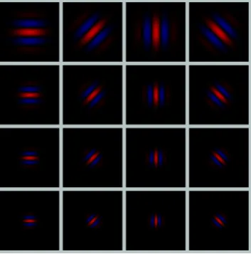
extract features in different orientations by using 16 different Gabor filters. The filters consist
of 4 different orientations, 0, 45, 90, 135 degrees and 4 different frequencies, 0.6, 0.7, 0.8, 0.9
for each orientation. The equation of the Gabor filters shows below;
2
( ' ')
( , , , , ) exp( ) sin( ')
2
' cos( ) sin( )
' sin( ) cos( )
freq x y
Gabor x y freq freq x
where x x y and
y x y
where x and y are the position in x-axis and y-axis, freq is the frequency of the filter, θ is an
orientation degree of the filter and
σ
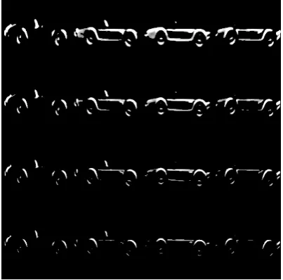
is the standard deviation. The examples of the extracted [image:14.595.210.387.162.341.2]features from Gabor filter in a 128x128x16 are shown in Figure 4.
Figure 3. 16 Gabor Filters for extracting features in the preprocessing component (Red color
shows the positive values and blue color shows negative values)
Freq\θ 0 45 90 135
0.6
0.7
0.8
0.9
Figure 4.The examples of extracting features by using 16 different Gabor filters.
[image:14.595.141.455.414.706.2]After Gabor processing, the system merges these extracted features together into one
large plane. The size of the plane is 512 x 512 pixels (128 x 4 = 512). The example of the plane
shows below (Figure 5). In the final step, these extracted images are normalized to [0-1] and
[image:15.595.197.399.191.390.2]sent as an input to the Feature Extraction Neural network
Figure 5. The example of the merging features in the preprocessor component
2.1.2 Feature Extraction Neural Network (FENN)
The Feature Extraction Neural Network is a hierarchical neural network consisting of
four layers. The layers process the information in different complexity from the simple
features in the first layer to morecomplex features in higher layers. Each layer of the network
contains 32x32 neurons with synapses (connections) from each neuron to other neurons in
previous layers (the neurons in the first layer connect to the preprocessor component). The
neurons and the synapses represent the structure of the brain which was first introduced by
McCulloch and Pitts in 1943. Every neuron has ability to modify their own synapses to learn
different functional tasks. The method of the synaptic modification that has been used in the
network is trace learning rule. The detail about this rule will be discussed in the Mathematic
Model of Trace rule section.
[image:16.595.152.445.246.468.2]2.2. Model of FENN Connection
Figure 6. The structure of the connections in FENN (Peerasathien, Woo, and Gaborski).
The connections of the FENN are determined by three parameters. The parameters are
the areas of the synaptic connections, the distributions of the synaptic connections and the
number of the connections for each neuron. As far as we know, the FENN network consists of
four layers and each layer contains 32x32 neurons. Each neuron from the higher layer has
connections from itself to the cells in the previous layer. The area of the connection of the
neuron connecting to the previous layer is limited by a constant diameter for each layer that a
neuron resides. The diameters of the connecting area are increasing from the lower layer to the
higher layer. The reason for increasing the size of the connection area is to make processing
information convergence in the highest layer. The structure of the connection area can be
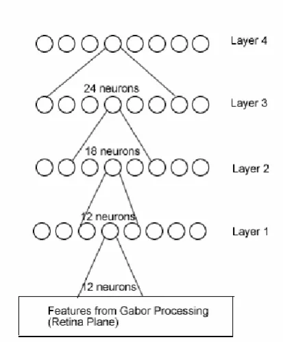
[image:17.595.211.418.170.420.2]found in Figure 7.The parameter of the diameters of each layer can be found in Table 1.
Figure 7. Example of the diameters of the connections between each layer.
In addition to the boundaries of the connection limited, but also the distribution of the
connections and the number of connections are also limited by some specific parameters. The
distributions of the connections are based on Gaussian probability distribution. The
distribution that I used is normal Gaussian distribution (
σ
= 1). Therefore, most connectionsare focused in the middle and lesser connections spread to the boundary of the area. The
example in Figure 8 shows the relationship between the Gaussian distribution of the
connections and other neurons in previous layer.
Figure 8. Example of the relation between the positions of the neurons and the Gaussian
distribution of the connections. Furthermore, we must be considered as the number of the
connections varies from layer to layer. The number of the connections in each layer used can
be found in Table 1.
Diameter of the connection area
The number of synaptic connections in an area
Layer 1 12 272
Layer 2 12 150
Layer 3 18 150
Layer 4 24 150
Table1. The parameters for the synaptic connections in FENN
2.2.1 Feature Extraction Network Process
The idea of Feature Extraction Network process is derived from Hebb’s hypothesis of
the leaning (Hebb, 1949)and competitive learning rule. These learning rules are based on the
real biological neuron processing and learning, with visual signal information.The process for
Feature Extraction Network will be in the next section.
2.2.1.1 Initialization Process
In the beginning state, the synaptic connections in the FENN are created and randomly
connected to the neurons in the previous layer. All synaptic connections are created with
weight values to represent their strength. The connection’s weights are initialized to the
connecting area randomly (based on connection diameters and the Gaussian distribution) and
normalized (for each neuron) to range between [0 1]. The weight normalizing procedure is to
ensure that the strength of the synaptic connection does not increase to infinite values. After
that, the FENN is ready to be trained for object categorization.
2.2.1.2 Training Process
The training process is the procedure to adjust all synaptic connection’s weights in the
entire FENN. The purpose of the weights adjustments is to make the network differentiate
images from different categories. This process can be divided into two sub-processes which
consist of activation computation, and updating computation. The training process starts by
feeding a training image to the system and on which the system will perform activation
computation. This activation computation will leave some hint values which will be referred to
as output values, for each neuron. Then, the system will perform updating computation. The
system will use the output values, from the activation computation, and update all the
connection’s weights. The activation and the weights updating process are described below.
2.2.1.2
a. Activation
In the activation part, the process begins with all neurons in the first layer receiving
input signals from the retina plane via the corresponding synaptic connections. The neurons
will perform mathematic operations (will be described more in Mathematic model of
Activation) to find output signals. After all the neurons in the first layer have produced their
output signals, these neurons will pass these signals as the inputs to the second layer. The
second layer will perform the mathematic operations (just as same as) in the first layer and
send the output signals to its succeeding layer and so on. The process of forwarding signals will
continue until all the neurons in the fourth layer produce their output signals.
I. Mathematic Model of Activation
According to the Feature Extraction Network architecture, we know that each neuron
in the previous layer has some synaptic connections with the neurons in the current layer.
Output signals from the neurons in a previous layer are sent through these synaptic
connections to the current layer. When the signals are sent from the neurons in the previous
layer to the neurons in the current layer, these signals (output signal from the previous layer)
perform linear combinations which is defined by
Figure 9. The diagram of connection of the neurons
( ) ( ) ( 1)
0
( ) l ( ) ( )
m
l l l
j ji i
i
v n w n y − n
=
=
∑
⋅ (1)where is the activation value for neuron j at time n, is the synaptic weights
connecting neuron i (previous layer) to neuron j (current layer),
( )
j
v n w nji( )
( )
i
y n is the output signal from
neuron i in previous layer and m is the number of connections of neuron j in the current layer l.
(the parameter of m in each layer can be found in Table1).
After completely finding all activation values for all neurons in the layer, the system
performs the “Local Lateral Inhibition” operation. This operation will inhibit some neuron’s
activation values and vise versa, enhance some neuron’s activation values. The purpose of the
operation is to prevent too many neurons from receiving input from a similar part of the
preceding layer responding to the same activity patterns (Rolls and Milward, 2000). The local
lateral inhibition is applied to the neuron’s activations by convoluting with a local lateral
inhibition filter I. The output from convoluting the activation values with local lateral
inhibition filter will be called “local inhibition activating values”. The equation of the filter I is
[image:21.595.204.391.467.639.2]shown below.
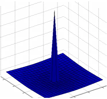
Figure 10. The example of local lateral inhibition filter
2 2 2 ( ) , 0 , 0
0
0
1
0
x y x yx x y
y
e
if x
or y
I
I
if x
and y
− + σ
≠ ≠
⎧
−δ
≠
≠
⎪
= ⎨
−
=
⎪
⎩
∑
,
0.
=
(2)where x and y are the distance from the center of the filter, δcontrols the contrast and
controls the width (Rolls and Milward, 2000).
σ
In the last step of the forward pass, the network transfers local inhibition activating
values to the sigmoid function. This process tries to map the group of neurons with the highest
local inhibition activating values to 1 and the rest of the activating neurons to 0. The sigmoid
function used in this network is
2 ( )
1 ( , , )
(1 x )
Sigmoid x
e β α
α β
= − −+ (3)
where α is a threshold and β is the slope of the graph. The valueα can be found by sorting all
outputs from local inhibition activating values in increasing order, and then choosing the
output at κth percentile asα (the parameters of κth
and β for each layer can be found in Table
2) . This forces the neurons in the same layer to compete among them and selects the group of
the highest activating neurons to become updated. If the local inhibition activating value of a
neuron is below the percentile then the output from the sigmoid will be 0 (no chance to
update in the next step). Otherwise, the output of the function will be between
th κ
(0-1].
th
κ
β
Layer 1 92 195
Layer 2 93 40
Layer 3 93 75
Layer 4 93 26
Table 2. The parameters of
κ
th andβ
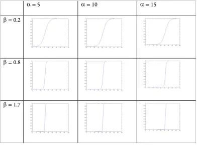
for each layer of FENNThe examples below illustrate how the parameters affect the output of the sigmoid
function. The x-axis and y-axis represent input value, x, and the output of the sigmoid
function.
α= 5 α= 10 α= 15
β= 0.2
β= 0.8
[image:23.595.102.495.190.481.2]β= 1.7
Figure 11. The examples of sigmoid function with different parameters
The results from the sigmoid function will be the final output signals for the neurons in
that layer and the input signals for the neurons in the succeeding layer. In addition, these
signals will be also hints for values for weight updating process in the next step
Figure 12. The summary of the signal flow in the activation process, forward computation, of
the feature extraction network
2.2.1.2b Weight Updating
When input signals flow from the preprocessing unit to each layer of the feature extraction
network, the network will adjust connection’s weights for learning these stimulus signals. The
changes of the weights are based on trace rule (Rolls and Milward, 2000) which comes from
the modification of Hebbian learning. Each time the signals are fed through a neuron, they
make some small changes in the synapse’s weights connecting to that neuron. If the neuron is
activated by the same feature signals at the exact time period, the connections of the neuron
will be strengthened (weights increasing). On the other hand, if the neuron receives different
feature signals or no activation in the neuron, the connections of neuron will be weaken
(weights decreasing).
I. Mathematic Model of Trace Rule
After completing processing activation computation, the neuron will begin to change
their own connection’s weights. In this step, the trace rule will be applied to determine the
weight for each connection. The trace rule equation is;
( ) (1 ) ( ) ( 1)
j j j
y n = − η ⋅y n + η⋅y n− (4)
where y nj( ) is the trace value at time n, yjis the output of neuron j and η is the constant
trace rate with the value between 0 – 1. From the equation, the new trace value (y nj( )) is
related to the current output value (y nj( )) and the previous trace value (y nj( −1)) in ratio
controlling by parameterη. If the system uses ηmore than 0.5, the new trace value,y nj( ), will
change mostly based on the previous trace value, y nj( −1). Vice versa, If the system uses η
less than 0.5 the new trace value will change mostly based on the new output value, . In
this paper, the value of used is 0.8 which gives the new trace value change mostly based on
the previous trace value(80% on the previous value and 20% on the current output value).
( )
j y n
η
Finally,the delta weights can be found for each connection from the new trace value,
( )
j
y n , and the current output value, y nj( ) by using the equation below:
Δwji = ⋅k y n y nj( )⋅ i( ) (5)
, where is a delta weights value in the synaptic connection which connecting from neuron
j to neuron i in the previous layer, k is a decay rate (for this paper, k=0.8) and
ji w
Δ
i
y is the output
value from the connecting neuron i in the previous layer (Rolls and Milward, 2000).The delta
weights Δwji will increase if multiplicationy nj( ) and y ni( ) has a high value compared with
other neurons in the previous layer that are connected to the neuron j. Otherwise, the will
decrease due to decay rate, k.
ji w
Δ
n yj y nj( −1) y nj( ) Δw nji( )
0 yj(0) 0 (1 ) (0)
j y
− η ⋅ k y⋅ j(0)⋅yi(0)
1 yj(1) (1 ) (0)
j y
− η ⋅ (1− η ⋅) yj(1)+ η⋅yj(0) k y⋅ j(1)⋅yi(1)
2 yj(2) (1 ) (1) (0)
j j
y y
− η ⋅ + η⋅ (1− η ⋅) yj(2)+ η⋅yj(1) k y⋅ j(2)⋅yi(2)
3 yj(3) (1− η ⋅) yj(2)+ η⋅yj(1) (1− η ⋅) yj(3)+ η⋅yj(2) k y⋅ j(3)⋅yi(3)
Table 3. The example of values of trace rule calculation in each iteration (n=1 to 3).
In addition, the trace rule can produce an infinite growth of the synaptic weights (when
neurons fire with high activating values all the time), which cannot be computed in this model
and is unrealistic in real biological synapses. Therefore, we need a mechanism to limit the
growths of the synaptic weights. Hence, in the final step, all the new synaptic weights
connecting with each neuron are normalized (for each neuron) to limit the growth of the
synaptic weights.
2.3. Back Error Propagation Network
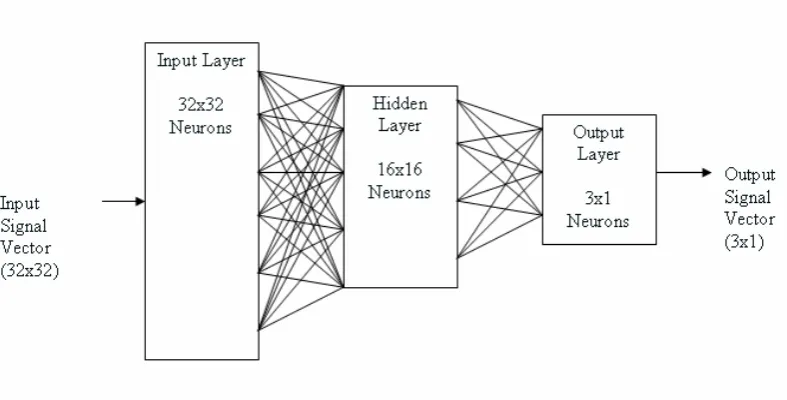
2.3.1 Model of Back-Propagation Connections
The back propagation neural network is the last network for processing in the system.
The main goal of this network is to classify the input images into groups. All neurons in the
input layer of the network are connected to the fourth layer of the FENN. The input signals of
Back-Error Propagation network (BEP) come from the output signals of the FENN’s fourth
layer. The input layer of BEP has 32x32 neurons same as the FENN network. However, in the
hidden layer the number of the neurons decreases to 16x16 neurons and the final layer or
output layer has only 3x1 neurons. The structure of the synaptic connections of the BEP is
quite different from FENN. The BEP is fully connected with the previous layer, which means
one neuron in higher layer has the synaptic connections with all neurons in the previous layer.
[image:27.595.79.473.460.660.2]An example of the architecture can be found below.
Figure 13. The architecture of the back-error propagation network
For the computational aspect, BEP has two types of computation: In Forward Computation,
the signals which flow from the first layer to the output layer, and in Backward Computation or
Back-Error Propagation, the signals flow from the output layer to the input layer, In the
Forward Computation , The signals propagate from the neurons in the input layer though the
neurons in hidden layers and then the final layer (layer by layer). All the synaptic weights
remain, no changes are made to the network. The forward signal-flow graph is shown below;
Figure 14. The signal-flow graph of Forward Computation (Haykin, 165)
The mathematic function for the forward computation is:
yj =ϕ( ( ))v nj (6)
where v nj( )is the activation value for neuron j at time n and ϕ( )• is the sigmoid function,
nonlinear function. The value can be found from the linear combination function
expanded in as equation (1). The sigmoid function,
( )
j v n
( )
ϕ • , that has been used in this system is
described below (Haykin, 168):
( ( )) 1 0 ( )
1 exp( ( ))
j j j
j
v n a and v n
a v n
ϕ = > − ∞
+ − ⋅ < < ∞ (7)
This sigmoid function ϕ( )• is similar to sigmoid function in FENN (Equation 3). The
purpose of this function is to make output convergence to 0 and 1 faster. This sigmoid
function has only two parameters, input value and constant, , for controlling sigmoid
slope.
( )
j
v n a
The Backward Computation is the computation for the signals propagating from the
output layer to the input layer, the opposite way of the forward signals. The backward signals
are also called “Error Signals” (Parker, 1987)and the network uses these signals to adjust the
synaptic weights layer by layer. The error signals can be found by comparing the actual output
of the network with the desired output. The error signals can be found by the following
equation.
e nj( )=d nj( )−o nj( ) (8)
where e nj( ) is the error signal at output neuron j at time n, djis the desired value at neuron j
and ojis the actual output value of the output neuron j.
We will use these error signals values to adjust the weights for each layer. The method
for adjusting the network is called Gradient Descent. The Gradient can be found by the
following equation;
( ) ' ( ) ( )
' ( ) ( 1) 1
( ) ( ( )) ( )
( ( )) ( ) ( )
L L
j j j
l
l l l
j
j j k kj
k
e n v n for neuron j in output layer L n
v n n w n for neuron j in hidden layer l ϕ
δ ϕ δ + +
⎧ ⋅
⎪
= ⎨ ⋅
⎪⎩
∑
(9)and the function ϕ'j( )• is the following equation;
ϕ'j(v( )jL ( ))n = ⋅a y nj( )[1−y nj( )] for the neuron in the output layer (10)
( ) ' ( )
( ) 2
exp( ( ))
( ( ))
[1 exp( ( ))]
l j l
j j l
j
a a v n
v n
a v n
ϕ = ⋅ − ⋅
+ − ⋅ for the neuron in the hidden layer (11)
In the final step of weights adaptation, the equation for weights updating can be found
below;
w n( )jil ( 1) w n( )jil ( ) α[w n( )jil ( 1)] ηδj( )l ( )n yil 1( )n
−
+ = + − + (12)
where η is the learning-rate parameter and
α
is the momentum constant. In this system I useη as 0.6 and
α
as 0.22.4. Summary of FENN Training Algorithm
The algorithm for learning in this network can be described as the following
procedure;
Initialize_FEN_Network
//starting process of FENN- Initial synaptic connections between FENN Network and Preprocessor Unit with
weights between 0-1 //make the connections between Preprocessor and FENN
- Initial synaptic connection between each layer of FENN with weights between [0-1]
- Normalize the synaptic weights in each neurons //prevent overflow computation
Initialize_BEP_Network
//starting process of Back-error Propagation Network- Initial the synaptic connections between BEP Network and the fourth layer of FEN
Network //make the connections from BEP to FENN
- Initial full synaptic connections between each layer. //make connection inside BEP
Activate_util_at( Image, iLayer)
//activation process of FENNat iLayer- Preprocess Image in Proprocessor Unit //process in Proprocessor unit first
- For i = 1 to iLayer //loop activation process from 1st layer in FENN until iLayer
- Activate(iLayer) //do activation process at iLayer
Train_FEN_Network_at( Image, iLayer)
//Training process of FENN at iLayer- Activate_util_at(Image, iLayer) //call Activate_until_at procedure and send Image and
//iLayer as parameters
- Update_Layer_at(Image, iLayer) //update weight at iLayer
Chapter 3
Experiment and Result
3.1 Cat and Dog Faces
3.1.1 Train FENN with Cat and Dog Faces
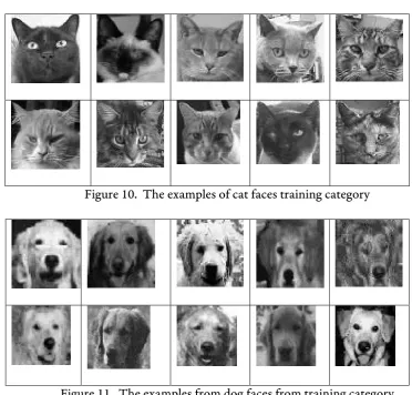
The system was trained to discriminate between cat and dog faces. The system was
trained by the database of 80 cat and 80 dog images, gray scale with 64x6 pixels. These images
are already known that they are either cat or dog face. The system will be trained by images in
categorical order. The examples of training images of cat category show in Figure 10 and dog
category in Figure 11.
[image:32.595.110.483.397.753.2]Figure 10. The examples of cat faces training category
Figure 11. The examples from dog faces from training category
In the first step, the system will randomly choose one training category for training the
initial layer, assuming that the cat category is used for training (Figure 10). When the cat
category is trained, the FENN will update the weights in the first layer according to trace rule
(Equation 5). If some similar cat features from the cat images are presented continuously to
the initial layer, the system will use the advantage of the trace rule to increase the strength
(weights) of the synaptic connections of the initial layer. Otherwise, if the features are
represented to the layer differently or non-continuously, the synaptic weights will be decay or
decrease.
When the first layer is trained by all cat images, all the weights remaining in the layer
now correspond to the cat features. After that,the system will reset trace values in the first
layer to 0 to start learning the new features from another category. Next, the dog category will
be trained to the FENN. The FENN will do the same process until all dog images are trained to
the first layer. Now both cat and dog features are trained to the FENN. The period of this
training with the two training categories is called “1 epoch”.
The first layer is trained with 100 epochs, and then the weights of the first layer’s
connections will be frozen, or no updating weights anymore. The next step is to train the
second layer. The second layer will use outputs from the frozen first layer as the second layer
inputs. The procedure of training the second layer is the same as the first layer. The second
was trained by randomly choosing one training category from the database. After training that
category to the second layer, the trace values are reset again before being trained with another
training category. The number of epochs for training the second layer is the same as the first
layer, 100 epochs. After all of the images are fed to the second layer, the weight of this layer will
be frozen with the same manner as the first layer. The process continues until the connections
of the fourth layer are frozen, and then the training procedure of FENN will be ended at this
step.
The examples below show the responding for each layer of the FENN with the training images
[image:34.595.257.340.189.275.2]from the cat and dog categories, when all the synaptic weights of the whole network are frozen.
Figure 12. The example of the training image of the cat category.
Figure 13. The output from each layer in FENN, after being tested by Figure 12.
Red indicates the highly responding output (close to 1). Yellow indicates the medium
responding neurons (between 0.5-0.8). Green indicates the non-responding neurons or
responding outputs that are very low. (Top Left) The output of the first layer. (Top right) The
output of the second layer. (Bottom left) The output of the third layer. (Bottom right) The
output for the fourth layer
[image:34.595.176.419.311.544.2]Figure 14. The example of the training image of the dog category.
Figure 15. The output from each layer in FENN, after being tested by Figure14.
Red indicates the highly responding output (close to 1). Yellow indicates the medium
responding neurons (between 0.5-0.8). Green indicates the non-responding neurons or
responding outputs that are very low (top left). The output of the first layer. (Top right) The
output of the second layer. (Bottom left) The output of the third layer. (Bottom right) The
output for the fourth layer.
The final step of the training process is to create the most shared features for each
category, which is called “complex features”. In this step, each of the training images was fed
into the frozen network. Then the highest frequency of the responding neurons in the fourth
[image:35.595.126.471.202.457.2]layer for each training category was measured. The term, “highest frequency” is evaluated at
the 95th percentile. Any frequency value higher than 95th percentile are recorded and compiled
as the complex features in the respective category.
[image:36.595.147.450.160.316.2]Cat complex features Dog complex features
Figure 16. The complex features (Left) for cat training category, (Right) for dog training
category.
3.1.2 Test Cat and Dog Faces with FENN
The system was tested by another database, called the testing database. This database
consists of 20 images of dog faces and 20 images of cat faces. These databases are different
from the images from the training section. Examples of the testing images are shown in Figure
17 and Figure 18:
Figure 17. The examples from cat faces in testing category
[image:36.595.68.514.541.733.2]Figure 18. The examples from dog faces in testing category.
The FENN will be tested with the training images in the fourth layer and comparing them with
the complex features of each category. The comparison between the example testing images
and the complex features from each category are show in Figure 19 and Figure 20. Figure 19
shows the cat testing image compared with cat and dog complex features. We can see that
many outputs of this cat image match with cat complex feature and a less match of dog
complex feature. Similarly, in the testing dog image, Figure 20, the output is more likely to
match to the dog complex feature matrix than the cat complex feature.
Example testing image from the
testing cat category
The responding of the 4th layer of
FENN
Cat Dog
Figure 19. (Top Left) The example of testing cat image chosen from testing database. (Top
Right) The responding of the neurons in the fourth layer of the FENN with the testing cat
image. (Bottom Left) The comparison between the responding neurons of the testing cat
image and complex feature of the training cat category (Bottom Right). The comparison
between the responding neurons of the testing cat image and complex feature of the training
dog category
*The red pixels are the correspondence between the testing image and complex features. The
yellow pixels are the response from the test image but no response from the complex features.
The green Pixels are the missing response from the test image for the complex features.
[image:38.595.106.494.69.482.2]Example testing image from the testing
dog category The responding of the 4th layer of
FENN
Cat Dog
Figure 20. (Top Left) The example of testing dog image chosen from testing database. (Top
Right) The responding of the neurons in the fourth layer of the FENN with the testing dog
image. (Bottom Left) The comparison between the responding neurons of the testing dog
image and complex feature of the training cat category (Bottom Right). The comparison
between the responding neurons of the testing dog image and complex feature of the training
dog category
*The red pixels are the correspondence between the testing image and complex features. The
yellow pixels are the response from the test image but no response from the complex features.
The green Pixels are the missing response from the test image for the complex features.
[image:39.595.94.502.68.476.2]In the next step, the number of responding neurons of all tested images (both cat and
dog testing categories) which correspond with the complex features of the cat and dog training
categories are shown. Figure 21 is the number of responded neurons to the testing cat category
compared with both cat and dog complex features. Figure 22 shows the number of responding
neurons to testing dog category compared with both cat and dog complex features. The y-axis
of both graphs shows the total number of the corresponded neurons and the x-Axis shows the
index of the testing images.
Test with all the testing cat images
Figure 21. The number of responded neurons of the tested 20 cat images comparing with
complex features. (Green line) The number of corresponded neurons to the dog complex features. (Red line) The number of corresponded neurons to the cat complex features.
Test with all the testing dog images
Figure 22. The number of responded neurons of 20 testing dog images comparing with
complex features. (Green line) The number of corresponded neurons to the dog complex features. (Red line) The number of corresponded neurons to the cat complex features.
3.1.3. Train Back Error Propagation Network
When the fourth layer synaptic connections are frozen, all the outputs of the fourth
layer are presented to the Back-error propagation (BEP) neural network. The BEP network
will initialize all synaptic connections between [-1 1] before starting any training. The
procedure of the BEP network is totally different from the procedure of FENN. The training
process of BEP begins with labeling all images from cat category with desired output vector [1
0 1] and all images from dog category with desired vector [0 1 0]. The system will first
randomly pick a training image either from the cat or dog category. The chosen image will be
processed in the preprocessor component and the frozen FENN before reaching BEP network
as an input. The BEP network will be trained by using back error propagation algorithm. The
error value is calculated by comparing the actual output vector of the BEP network and desired
vector for that image’s category. Every time that the network is trained, the network will adjust
the weights of synaptic connection in all layers from the output layer to the input layer
layer-by-layer. The continuous adjustment of BEP network make the BEP produce less error output
or tend to have less error output at every epochs. The errors of BEP network are measured by
Error-Mean-Squared value by comparing the actual output and the desired output for the
testing images. The EMS graph is represented in Figure 23 after 100 epochs. At the end of the
BEP training, the network will be frozen same as FENN. Now the whole network system is
[image:42.595.199.399.315.476.2]ready to categorize the testing set. The results are shown below;
Figure 23. Mean-Squared Error graph of the BEP
3.1.4 The Result of classification of cat and dog faces
Test Images Output Vector
Desired Cat Output Vector [1 0 1] Desired Dog Output Vector [0 1 0]
[ 0.96784691684662 0.0298604567591284 0.967780953419655 ]
[ 0.808654146731156 0.193775062928928 0.810705977968617 ] [ 0.00754134248377787 0.989143744690816 0.00999103943572717 ]
[ 0.0141790736335504 0.987664666208226 0.0129025723749382 ]
Images\ Results Classify as Cat Classify as Dog Correctness %
Cat Images 20 0 100%
Dog Images 1 19 95%
Table 4. Summary of Cat and Dog faces classification. (Other results can be found in Appendix I)
3.2.1 Car with Size Invariance
The procedure of the training FENN in this section is similar to the procedure of
training cat and dog face. Except we train FENN with only one category which is car category
with different sizes (Figure 24). Then BEP network will be trained with various sizes of car in
background and background images (Figure 25) for making the system classify images
with/without cars.
Figure 24.The examples of car images for training the FENN.
Example of Training Set of BEP Network
Figure 25. The examples of training set of car with different sizes images that used to train BEP Network with desired output vector [0 1 0]
Figure 26. The examples of training set of background images that used to train the BEP Network with desired output vector [1 0 1]
3.2.2 The Result of classification of Car with Size Invariance and
Background
Tested Images Output Vector
Desired Car category [0 1 0]
Desired Background category [1 0 1]
[ 0.00131129525251674 0.998737326089361 0.00115486102794309 ]
[ 0.00949948886090213 0.990354534265279 0.00930097035040287 ]
[ 0.885260759720194 0.0851067957046222 0.925031120954687 ]
[ 0.000123605022367777 0.999873666489406 0.000163150633651208 ]
Images\ Results Classify as Car Classify as Background Correctness %
Car Images 14 6 70%
[image:45.595.67.495.131.503.2]Background Images 3 7 70%
Table 5. Summary of Car with size invariance classification. (Other results can be found in Appendix II)
3.3.1 Car with Rotation Invariance
In this testing part, the system was trained to recognize a car with different
[image:46.595.120.478.195.435.2]orientations. The training set of FENN shows in Figure 27 and the training sets of BEP show in
Figure 26 and Figure 28.
Figure 27. The training set of FENN for rotation invariance
Figure 28. The training set of BEP for rotation invariance
[image:46.595.114.482.465.734.2]3.3.2 The Result of classification of Car with Rotation Invariance and
Background
Tested Image Output Vector
Desired Car category [0 1 0] Desired Background category [1 0 1]
[ 0.728102731220183 0.252897655361728 0.778945371560569 ]*
[ 0.457237935527262 0.50530959812553 0.416905661877368 ]
[ 0.73295255107279 0.204610049442978 0.772291769529087 ]
[ 0.803291409325187 0.177796521122199 0.83944855512533 ]
*Wrong classification
Images\ Results Classify as Car Classify as Background Correctness %
Car Images 11 1 90.9%
[image:47.595.67.495.135.563.2]Background Images 3 7 70%
Table 6. Summary of Car with rotation invariance classification. (Other results can be found in Appendix III)
3.4.1 Car with Position Invariance
In this testing part, the system was trained to recognize a car with different position.
[image:48.595.148.448.167.399.2]The training set of FENN shows in Figure 29.
Figure 29. The training set of FENN for translation invariance
3.4.2 The Result of classification of Car with Translation Invariance
and Background
Tested Image Output Vector
Desired Car category [0 1 0]
Desired Background category [1 0 1] [ 0.929563003955722
0.0517581762961036 0.944550079477863 ]*
[ 0.0894011291618318 0.922182595028458 0.114840724541637 ]
[ 0.866981151456251 0.123257373191556 0.859489742898194 ]
[ 0.0162461312866995 0.981999694017879 0.0148910774563106 ]*
*Wrong Classification
Images\ Results Classify as Car Classify as Background Correctness %
Car Images 8 12 40%
[image:49.595.63.496.70.271.2]Background Images 5 5 50%
Table 7. Summary of Car with size invariance classification. (Other results can be found in
Appendix IV)
3.5.1 Car with all Invariance
In this testing part, the system was trained to recognize a car with different
orientations and scales. The training set of FENN shows in Figure 24 and Figure 27 for scale
invariance and rotation invariance respectively. The training sets of BEP show in Figure 25,
Figure 26 and Figure 28
3.5.2 The Result of classification of Car with Rotation Invariance, Size
Invariance, Position Invariance and Background
Tested Image Output Vector
[image:49.595.70.497.599.754.2]Desired Car category [0 1 0] Desired Background category [1 0 1]
[ 0.00335647041698926 0.996839814509679 0.00344293229620998 ]
[ 0.0308976065556976 0.979137071552084 0.014550470828915 ]
[ 0.0378490627662957 0.967533755973145 0.0299702136390872 ]
[ 0.0223966575256114 0.979978594576491 0.019756532717237 ]
[ 0.00570342452860919 0.99354105047225 0.00686954034030893 ]
[ 0.822300973953372 0.168583446615338 0.748539715282723 ]
[ 3.64333096031036E-5 0.99993288400426 4.30812056281187E-5 ]*
[ 0.435566579540336 0.637663772415885 0.329488131786573 ]
*Wrong Classification
Images\ Results Classify as Car Classify as Background Correctness %
Car Images 31 10 75.6%
[image:51.595.76.514.73.163.2]Background Images 6 5 45%
Table 8. Summary of Car with all in variances classification. (Other results can be found in Appendix V)
3.6 Results from Integrated with
a Biologically Inspired Focus of
Attention Model
System.
In the last part of this chapter, this system was integrated with another vision
recognition system, a biologically inspired focus of attention model by Daniel Harris (Harris,
2007) and it extends the ability to recognize cars from video files and to find the object’
positions in the scenes. Harris’s system extracts interesting areas from video stream such as
road signs, peoples, animals and cars. The system is a blind extracting system, it doesn’t know
“what” the objects are. It only knows “where” the objects are in the scene. Therefore, the
integration of Harris’ system to this system will further maximize the function of this system
by recognizing both the “what” and “where” of the objects.
Figure 30. The example frame before extracting interesting area by Harris’s system.
The system was trained by using the same dataset and method as section 3.2 in both FENN
and BEP networks. After completed training the system was tested by segmentation of the area
[image:51.595.242.391.551.663.2]from Harris’s system. The results of interesting areas extracting by Harris’s system (left) and
the final classification vector by Biologically Inspired Object Categorization system (right).
Tested Image Output Vector
Desired Car category [0 1 0] Desired Background category [1 0 1]
[ 0.0845976807106649 0.931954326666755 0.0768767815351636 ]
[0.373440 0.088477 0.617099 ]
[0.694197 0.019668 0.558695 ]
Images\ Results Classify as Car Classify as Background Correctness %
Car Images 5 0 100%
[image:52.595.63.495.163.528.2]Background Images 0 4 100%
Table 9. Summary of Car with all in variances classification. (Other results can be found in
Appendix VI)
Chapter 4
Conclusion and Future Work
This system shows an ability of the biologically inspired system that can classify the
real world images into correct categories, even the images has a wide range of features. The cat
and dog faces are an example of the wide range of features: different textures of fur, various
shapes of face and numerous positions of eyes, ears and mouths. The system applies the
features extraction algorithm to find the common features among the same categories and
discriminate features between the two categories and finally categorizes by using the BEP
network. The results are 100% accurate for categorizing cat faces and 95% for dog faces.
The next experiment of car detection is another challenging task to answer the
question, “car” or “no car”. The system has to detect the car with a variety of sizes, positions
and orientations in the urban scene. Moreover, the scenes are also very complex and have
wider range of unknown features of buildings, trees, road and etc, In other words, an infinite
features would have to be recognized. However, the system still gives satisfying results about
70% correct classification for size and rotation testing although there is a failure in translation
invariance problem, with an unacceptable testing result of 40 % in two categories classification.
The future work for this system is to create a powerful preprocessing unit which can extract
useful information from image scenes and ignore other non-related features. One of the
prominent methods is by replacing Gabor filter with a dynamic filter such as sparse coding.
The coding extracts features by finding correlation among images and provides more
information to be used in the preprocessor unit. For FENN unit, the trace rule, which is used
as the main feature extraction algorithm, requires long period of training. The alternative way
to replace the algorithm can be used with some simple calculation methods such as finding
Mode (statistical method) among the training images. Then, the highest frequency features
that can be found over the FENN layer are selected to be compare with each testing image.
The reason that I suggest this method because I found that trace rule is quite similar to the
Mode method. The classifier network, the BEP network, is the last one that should be
improved by replacing BEP Network with other high efficient methods. ID3 is one of the most
powerful methods for classification. I believe that if we use these methods the system will give
higher accuracy with faster training speed than BEP network.
Works Cited
Duetsch, J. A. “A Theory of Shape Recognition.” British Journal of Psychology 46 (1955):
30-47.
Enroth Cugell, C, and J. G. Robson. “The constrast sensitivuty of retinal ganglion cells of the
cat.” Jornal of Physiol 187 (1966): 517-552.
Foldiak, P. “Learning invariance from Transformation Sequence.” Neural Comput 3 (1991):
194-200.
Fukushima, K. “A Self-Organizing Neural Network Model for a Mechanism of Pattern
Recognition Unaffected by Shift in Position.” Biological Cybernetics 36.4 (1980):
93-202.
Fukushima, K, S. Miyake, and T. Ito. “A Neural Network Model for a Mechanism of Visual
Pattern Recognition.” Cybernetics 13 (1983): 826-834.
Fukushima, Kunihiko, and Sei Miyake. “Neocognitron: A New Algorithm for Pattern
Recognition Tolerant of Deformations and Shifts in Position.” Pattern Recognition
15.6 (1982): 455-469.
Harris, Daniel. A Biologically Inspired Focus of Attention Model. MS thesis. Rochester Inst.,
2007. Rochester: n.p., n.d. 2 Mar. 2008 <https://ritdml.rit.edu/dspace/handle/1850/5712>.
Haykin, Simon. Neural Networks. 1999. Ed. Simon Haykin. New Delphi: Prentice Hall of
India, 2006. Neural Networks: A Comprehensive Foundation. N.p.: Prentice Hall,
1998.
Hebb, D. O. The Organization of Behavior. New York: Wiley, 1949.
Hubel, D. H., and T. N. Wiesel. “Receotive Fields, Binocular,Interaction and Funtional
Architecture in the Cat’s Visual Cortex.” Journal of Physiology 160 (1962): 106-154.
Kandel, E. R., J. H. Schwartz, and T. M. Jessell. Principles of Neural Science. 4th ed. New York:
McGraw-Hill, 2000.
Koffka, K. “Principles of Gestalt Psychology.” Harcourt-Brace (1935).
Kohonen, T. “Self-Organized Formation of Topologically Correct Feature Maps.” Biological
Cybernetics 43 (1982): 59-69.
Kuffler, S.W. “Discharge patterns and functional organization of mammalian retina.” Journal
of Neurophysiology 16.1 (1953): 37-68.
Logothetis, N. K., et al. “Neurons to Novel Wire-Objects in Monkeys Trained in an Object
Recognition Task.” Neuroscience 19.23 (1993).
Olshausen, B. A., and D. J. Field. “Sparse Coding with an Overcomplete Basis Set: A Strategy
Employed by V1.” Vision Research 37 (1997): 3311-3325.
Palmer, S. E. Psychology of Perceptual Organization: A Transformation Approach, in Human
and Machine Vision. New York: Academic Press, 1983.
Parker, D. B. “Optimal Algorithms for Adaptive Networks: Second Order Back Propagation,
Second Order Direct Propagation, and Second Order Hebbian Learning.” IEEE 1st
Interantional Conf. on Neural Network 2 (1987): 593-600.
Peerasathien, Theparit, Myung Woo, and Roger Gaborski. “Biologically Inspired System for
Object Categorization in Cluttered Scenes.” Applied Imagery Pattern Recognition
(Oct. 2007).
Riesenhuber, Maximilian, and Tomaso Poggio. “Hierarchical models of object recognition in
cortex.” Nature Neuroscience 2 (1999): 1019-1025.
Rolls, E. T., and T. Milward. “A Model of Invariant Object Recognition in the Visual System:
Learning Rules, Activation functions, lateral inhibition, and Information-Based
Performance Measures.” Neural Comput 12 (2000): 2547-2552.
Serre, T, and M. Riesenhuber. “Realistic Modeling of Simple and Complex Cell Tuning in the
HMAX Model, and Implications for Invariant Object Recognition in Cortex.” CBCL
Paper (2004).
Stringer, Simon M., and Edmund T. Rolls. “Invariant Object Recognition in Visual System
with Novel Views of 3d Objects.” Neural Computation 14 (2002): 2585-2596.
Ungerleider, L. G., and J. V. Haxby. “’What’ and ‘where’ in the human brain.” Curr Opin
Neurobiol 4.4 (Apr. 1994 ): 157–165.
Wallis, G. “Using Spatio-Temporal Correlation to Learn Invariant Object Recognition.”
Neural Network 9 (1996): 1513-1519.
Wallis, G., and E. T. Rolls. “A Model of Invariant Object Recognition in the Visual System.”
Progress in Neurobiology 51 (1997): 167-194.
Appendix
I. Final Result from the Entire Network
Test Images Output Vector
[ 0.0149574143759123 0.986097146397701 0.0172635142157268 ] [ 0.0164512758205673 0.986075209215739 0.0135553685172644 ] * Wrong classification
II. The Result of classification of Car with Size Invariance and
Background
Tested Images Output Vector
Desired Car category [0 1 0]
[ 0.00131129525251674 0.998737326089361 0.00115486102794309 ]
[ 0.00949948886090213 0.990354534265279 0.00930097035040287 ]
[ 0.0866038575036774 0.912180902695252 0.0779660346671882 ]
[ 0.00232631696118088 0.997791243028115 0.00261413336765878 ]
[ 0.000320680579091279 0.999724293511722 0.000229089781810894 ]