Rochester Institute of Technology
RIT Scholar Works
Theses
Thesis/Dissertation Collections
8-18-2006
Tool for the identification of differentially expressed
genes using a user-defined threshold
Renikko Alleyne
Follow this and additional works at:
http://scholarworks.rit.edu/theses
This Thesis is brought to you for free and open access by the Thesis/Dissertation Collections at RIT Scholar Works. It has been accepted for inclusion
Recommended Citation
Thesis
Committee
Committee Chair
Dr. Gary R. Skuse Director of Bioinformatics
Department of Biological Sciences College of Science
Rochester Institute of Technology
Committee Member
Dr. James Halavin Professor
Department of Mathematics & Statistics College of Science
Rochester Institute of Technology
Committee Member
Professor Paul Tymann Department Chair
Department of Computer Science
Abstract
Microarray and 2D gel experiments are used for the large scale measurement, and
comparison of gene expression. Since these experiments generate large and complex amounts
of data, a great challenge the researcher faces is trying to find ways to analyze this data. This
paper focuses on the tool DiffExpress, which was designed to make the gene expression
analysis process easier. One of the main features of DiffExpress is the user defined threshold
which allows users to set their personal restriction of the expression change at which genes
are differentially expressed. DiffExpress also makes use of graphs such as the Scatter Plot, Box
Acknowledgements
I would like to offer special thanks to my thesis committee who helped in all aspects of this
thesis and provided guidance throughout. Appreciation goes to Dr. Skuse who formulated the
fantastic idea for this thesis. Without him, I would still be working on a thesis project that
was impossible to finish. I am very grateful for Dr. Halavin’s extensive input, and assistance.
He was always willing to meet with me to discuss a new idea or assist in solving any problems
that arose. He made working on this thesis interesting and challenging, with his excellent
suggestions and his creativity. I would like to thank Professor Tymann for his help with the
programming aspects and the written thesis. I also greatly appreciate the constructive
Table of Contents
1 INTRODUCTION ... 1
1.1 Genes and Proteins... 1
1.2 Gene Expression: Genome to Proteome... 1
1.3 mRNA and Protein Expression Levels ... 3
1.4 DNA Microarrays ... 4
1.5 cDNA Microarrays ... 5
1.6 Oligonucleotide Arrays ... 9
1.7 2D Gels and Mass Spectrometry ... 11
1.8 Expression Data Analysis ... 11
2 RATIONALE ... 16
3 METHODS... 18
3.1 Input... 18
3.1.1 Input Data ... 18
3.1.2 Missing Values ... 19
3.1.3 Input Data Limitations ... 20
3.2 Analysis ... 23
3.2.1 Advanced Data Information... 23
3.2.2 User Defined Threshold ... 28
3.2.3 Expression Change... 29
3.3 Output ... 34
3.3.1 Expression Change Detection ... 34
3.3.2 Graphs ... 36
3.3.3 Expression Profile ... 44
4 Implementation... 45
4.1 Java ... 45
4.2 JFreeChart ... 45
4.3 Packages ... 45
4.3.3 Datasets... 46
4.3.4 Frames ... 47
4.3.5 Graphs ... 54
5 PROBLEMS FACED... 55
5.1 Missing Values ... 55
5.2 Infinity Values ... 55
6 FUTURE WORK ... 56
6.1 Preprocessing... 56
6.2 Volcano Plot Implementation ... 56
6.3 Clustering... 56
6.4 Identification of Differentially Expressed Genes... 57
REFERENCES ... 58
List of Tables
Table 1: Simplified Example of an Expression Data Matrix... 12
Table 2: Expression Change Calculation - raw oligonucleotide microarray data... 31
Table 3: Expression Change Calculation - raw cDNA microarray data ... 32
Table 4: Expression Change Calculation - log transformed oligonucleotide microarray data.. 33
Table 5: Expression Change Calculation - log transformed cDNA microarray data ... 33
Table 6: Summary of Expression Change and Types of Regulation ... 34
List of Figures
Figure 1: Steps in Gene Expression and its Regulation ... 2
Figure 2: cDNA Microarray Experiment Example... 7
Figure 3: Simplified example of some cDNA signals in a digital image. ... 8
Figure 4: Actual Representation of the colors of a microarray... 8
Figure 5: Oligonucleotide Array Experiment Example ... 10
Figure 6: Examining the effects of experimental conditions ... 13
Figure 7: Comparing different cell populations ... 14
Figure 8: Workflow of DiffExpress ... 18
Figure 9: Example of the format for Input Data... 22
Figure 10: DiffExpress - Advanced Data Information Options Window ... 23
Figure 11: One-to-many comparison... 25
Figure 12: DiffExpress - One-to-many comparison ... 25
Figure 13: Paired Groups Comparison... 26
Figure 14: DiffExpress – Paired Groups Comparison... 27
Figure 15: Unpaired Groups Comparison ... 27
Figure 16: DiffExpress - Unpaired Groups Comparison ... 28
Figure 17: DiffExpress - Threshold Range... 28
Figure 18: DiffExpress - Expression Change Option... 29
Figure 19: DiffExpress - Output Display... 35
Figure 20: DiffExpress - Example of output text file... 36
Figure 21: DiffExpress - An example of a Scatter Plot with an outlier. ... 37
Figure 22: DiffExpress - Box and Whiskers Plot ... 38
Figure 23: DiffExpress - Scatter Plot... 39
Figure 24: DiffExpress - RA Plot... 41
Figure 25: Volcano Plot ... 42
Figure 26: DiffExpress - Gene Expression Profile ... 44
Figure 27: DiffExpress - Main Application Window ... 48
Figure 28: DiffExpress - cDNA Scatter Plot Options Window ... 49
Figure 30: DiffExpress - Expression Levels Basic Plot Options Window ... 51
Figure 31: DiffExpress - Outliers and Box & Whiskers Plot: Plot Graphs... 51
Figure 32: DiffExpress - Outliers and Box & Whiskers Plot: Display Outliers Information .... 51
Figure 33: DiffExpress - Pearson Correlation Coefficient Options Window ... 52
Figure 34: RA Plot Error Frame ... 52
1 INTRODUCTION
1.1 Genes and Proteins
The gene, often defined as the basic unit of heredity, is a segment of DNA which
codes for a protein or RNA molecule. Cells in the body contain identical genes, but in each
cell, not all of these genes are expressed. At any given time, a gene in one cell may be active
while in another cell this same gene may be inactive. The type of cell and the cell’s
environmental conditions are some factors that may determine which genes are expressed.
The protein is the product of gene expression. It is one or more polypeptides folded
into a specific 3-dimensional conformation. A protein’s function is dependent on its specific
3-dimensional conformation which in turn is dependent on the sequence of its amino acids.
There are tens of thousands of proteins in the body, each with a specific function and
structure. It is the protein (not the gene) that carries out most of the work necessary for the
cell to function normally.1
1.2 Gene Expression: Genome to Proteome
Gene expression (also known as protein expression) is the process by which a gene is
turned on, and its information is used in RNA production (RNAs other than mRNA which are
a product of transcription) or protein production (transcription followed by translation). A
gene is said to be expressed when its mRNA or protein are detected. When looking at gene
expression, we want to identify which genes are expressed and the amount of expression.
Transcription (Figure 1) is the process by which a strand of DNA is used as a template
occurs and modifies the primary transcript, creating a mature mRNA. In translation the
mature mRNA is used to produce a polypeptide.
Figure 1: Steps in Gene Expression and its Regulation
Cells are able to regulate gene expression by adjusting the rate of gene transcription
and translation, hence determining which genes are being expressed and the quantity.
Alterations in this cell regulation mechanism can cause over or under expression of genes, DNA
Pre-mRNA
Protein
RNA processing Transcription
mRNA
causing diseases or other damage. Regulation of gene expression usually occurs at the level of
transcription. This involves the binding of transcription factors to the promoters and
enhancers of genes, helping to activate or inactivate these genes. Gene expression may also
be regulated at the level of translation, although it does not occur as much as regulation at the
level of transcription. RNA interference, riboswitches and proteins are some of the factors of
gene expression regulation.2
1.3 mRNA and Protein Expression Levels
Gene expression analysis involves the measurement and analysis of gene expression,
using mRNA expression levels and/or protein expression levels in a sample. It is easier to
measure mRNA expression, but it is believed that measuring the variation in protein
expression patterns is more accurate with respect to the analysis of gene expression.
Microarray analysis allows researchers to determine which genes in a sample are
activated.3 In a sample, only active genes produce mRNA, so based on the mRNA present a
gene expression profile can be constructed to obtain a map (list) of the genes that are active or
inactive in the sample.3 mRNA levels can give a lot of information about the state of the cell
and its gene activity. Up-regulation and down-regulation of mRNA is believed to be
associated with functional changes in the cell. This is true in some cases, but it is usually the
proteins that affect most of the cell’s processes.
Protein expression analysis is a collection of techniques that researchers use to
determine which proteins are being produced in a sample and are functional. A protein
in a sample at a given time.1 Because of the many stages between mRNA expression and
protein expression, there is not always a strong correlation between mRNA and protein
expression. A large quantity of mRNA may be produced, yet the protein produced may not
display any over-expression.1
1.4 DNA Microarrays
The DNA microarray is used for the simultaneous measurement and examination of
thousands of mRNA expression levels (level of transcription) in a sample. The microarray is
simply a microscope slide, nylon membrane or silicon chip upon which thousands of genes
(DNA targets) are spotted, printed or synthesized.4
DNA microarray technology takes advantage of the fact that mRNA molecules
hybridize to their complementary DNA sequence.4 Target DNA is immobilized to a solid
support to create the microarray. Researchers use the location of the each spot on the
microarray to identify a specific gene, therefore it is imperative that these targets are
immobilized to the array in an orderly fashion.4 mRNA is isolated from samples and reverse
transcribed into cDNA which is labeled and used as a probe. These probes are incubated with
the microarray and bind to their complementary target DNA. By measuring the amount of
mRNA adhered to each microarray spot, the expression level each gene can be obtained.
DNA microarrays are commonly used for comparing gene expression in different cell
populations. For example, the use of microarrays for the comparison of healthy cells/tissues
Another widely used application is in the examination of the effects of experimental
conditions (e.g. drug response or time-course studies) by measuring and detecting the changes
in gene expression levels of a sample under different conditions.
Two predominantly used types of microarrays are cDNA (complementary DNA)
arrays and oligonucleotide arrays. cDNA microarrays produce a ratio of red (cy5) channel to
green (cy3) channel for each spot. The ratio is indicative of the relative expression change for
each gene under two different experimental conditions, and may be raw or log-transformed.
Unlike cDNA microarrays, oligonucleotide microarrays do not produce ratios, but instead
produce an absolute intensity for each spot.
1.5 cDNA Microarrays
cDNA microarrays use DNA fragments which are 500 to 1500 base pairs long, and can
be used to measure the change in expression between two different samples, for example a
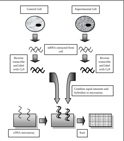
sample taken from healthy tissue and a second sample taken from diseased tissue. Figure 2
illustrates an example of the basic method for conducting an experiment using a cDNA
microarray. The fundamental steps in this method are as follows 6:
1. DNA fragments (also known as probes) are spotted and immobilized onto the
microarray (usually a glass slide).
2. mRNA from two cell samples (usually a control cell and an experimental cell) in
3. To differentiate between the two samples, the cDNA from each sample is labeled
with either a red (Cy5) or green (Cy3) fluorescent dye. For example the control
sample’s cDNA may be labeled with Cy5 while the experimental sample’s cDNA is
labeled with Cy3, or vice versa.
4. The two pools of fluorescently labeled cDNA are combined in equal amounts and
applied to the microarray.
5. The labeled cDNA from each sample compete to hybridize to its complementary DNA
fragment on the microarray. The sample that contains more of an mRNA transcript
for a specific gene will have a better chance of hybridizing to that gene.
6. The microarray is washed to eliminate any cDNA that was not hybridized.
7. A digital image (e.g. Figure 4) is created of the red and green signals and computer
software is used to calculate the red to green fluorescence ratio for each spot. The
signals from a spot indicate the relative abundance of the corresponding mRNA in the
two cell populations. For example, for a given gene, if the control sample was labeled
with Cy3 and it contains more mRNA transcript than the experimental sample
labeled with Cy5, then the probe (spot) on the array will be green. If, on the other
hand, the experimental sample’s mRNA content exceeds that of the control sample’s
mRNA content, then the probe will fluoresce red. If both the samples have the same
and the probe will fluoresce yellow. If nothing has hybridized to the spot, then there
[image:18.612.110.543.141.634.2]will be no signal and the probe will be black.7
Figure 2: cDNA Microarray Experiment Example
Combine equal amounts and hybridize to microarray mRNA extracted from
cell
Reverse transcribe
and label with Cy3
Reverse transcribe
and label with Cy5
cDNA microarray Scan
Experiment 1 Experiment 2 Experiment 3
Gene A Red Green Red
Gene B Black Red Yellow
[image:19.612.109.313.296.505.2]Gene C Yellow Black Green
Figure 3: Simplified example of some cDNA signals in a digital image.
Red indicates that Cy5 > Cy3, Green indicates that Cy3 > Cy5, Yellow indicates that Cy5 = Cy3 and Black indicates that no hybridization of the probe to the target occurred.
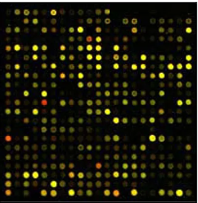
Figure 4: Actual Representation of the colors of a microarray
1.6 Oligonucleotide Arrays
Unlike cDNA microarrays, oligonucleotide arrays use short 25 base-pair DNA
fragments as their probes and only one sample is hybridized to the array. This type of array
can be used to measure the RNA content in a sample, or it can be used to compare two
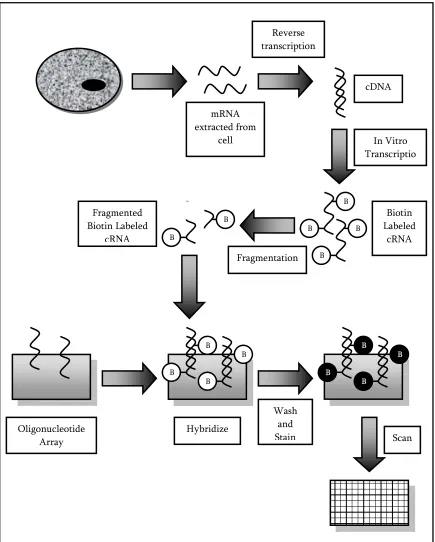
different samples (these samples must be hybridized on separate arrays). Figure 5 illustrates
an example of a typical oligonucleotide array experiment. The basic steps in this method are
as follows 6:
1. UV masks and photo-activated chemistry are used in cooperation to immobilize the
DNA oligonucleotides on the microarray.
2. mRNA is extracted from the sample and reversed transcribed into cDNA.
3. cDNA is transcribed into cRNA and labeled (usually with biotin).
4. The labeled cRNA is fragmented and hybridized to the oligonucleotide array.
5. The array is washed to remove any excess cRNA, and stained to visualize the amount
Figure 5: Oligonucleotide Array Experiment Example Hybridize mRNA extracted from cell Wash and Stain Reverse transcription Oligonucleotide
Array Scan
1.7 2D Gels and Mass Spectrometry
Like DNA microarrays, 2D gels and mass spectrometry are high-throughput
techniques, but unlike DNA microarrays, 2D gels and mass spectrometry are associated with
proteins and not mRNA. Measuring protein expression is different from mRNA expression
measurement. Global changes in protein expression can be detected by the use of 2D gels and
mass spectrometry. 2D gels are used to separate proteins in a sample while mass spectrometry
is used for the large-scale protein identification and the measurement of expression of the
proteins in the sample (and find differences in protein expression between two of more
samples).1 In order to find proteins that are differentially expressed, data from different
samples or from one sample under different conditions are compared. Given two or more
samples, comparing their mass spectra can provide information about variations in the
protein expression level patterns between them. There is software available that provides
features for spot detection, spot quantification and comparison of multiple gels.
1.8 Expression Data Analysis
Table 1 shows a very basic layout of an expression data matrix. An expression matrix
is a table of expression levels in the case of oligonucleotide microarray data, or expression
level ratios in the case of cDNA microarray data. Actual results usually contain thousands of
gene/ spot id data. The columns represent samples and experiments while the rows represent
genes corresponding to an mRNA or protein. Each cell (bordered by the bold shaded squares
in Table 1) gives the expression level (oligonucleotide microarrays) or ratio of expression
levels between two samples (cDNA microarrays) of a gene or protein (based on either mRNA
would either be the mRNA level or protein level of gene C in sample 2.
Samples
1 2 3
A Expression Level A1 Expression Level A2 Expression Level A3
B Expression Level B1 Expression Level B2 Expression Level B3
Gene
C Expression Level C1 Expression Level C2 Expression Level C3
Table 1: Simplified Example of an Expression Data Matrix
If we want to determine how similar or dissimilar the expressions of two genes are,
we compare the rows (expression profiles). Co-regulation of the genes can also be
determined, i.e. if gene A is regulated (or down-regulated), are genes B or C also
up-regulated (or down-up-regulated).
If we want to determine if samples are related or unrelated, we compare the columns.
If they are unrelated, genes that cause this dissimilarity can be found through the comparison.
Alterations in gene expression can occur from drugs, changes in the environment, etc.
Researchers may want to examine differences in expression between sample 1 and 2 given
1. Sample 1 and sample 2 are taken from the same sample under different experimental
conditions (drug response experiment e.g. drug treatment, radiation). For example in
drug response experiments, sample 1 may be a cell treated with specific drug while
sample 2 may be the same cell treated with a different drug (Figure 6). One drug may
cause some changes in the expression of certain genes of the cell while the other drug
may alter the expression of completely different genes. Comparison of these two
samples will then provide insight into which drug could possibly be successful in
treating a specific condition.
Figure 6: Examining the effects of experimental conditions
Sample 1 is taken from the tissue treated with drug 1, while Sample 2 is taken from the tissue treated with drug 2.
Dosage 1
Tissue
Sample 1 Sample 2
2. Sample 1 is a normal cell while sample 2 is a diseased cell. A simple example of this is
sample 1 is a cell taken from normal tissue while sample 2 is a cell taken from the
tissue of a tumor (Figure 7). Comparing these two samples, researchers may find
genes/proteins that show a significantly different level of expression in the tumor cell.
Discovering these significant genes or proteins can assist in providing a clue in
determining disease susceptibility and will ultimately be useful in the diagnosis and
treatment of various diseases.
Figure 7: Comparing different cell populations
Sample 1 is taken from normal tissue while Sample 2 is taken from diseased tissue
Sample 1 Normal
3. Sample 1 and Sample 2 are taken from a cell or tissue at different times. An
experiment of this type is known as a time-course experiment and is basically the
2 RATIONALE
The introduction of microarray technology has been a significant asset to scientific
research by saving researchers time and effort, but these researchers are faced with the
challenge of the analysis of the microarray expression data. One challenge is finding and
making sense of the gene expression patterns which result from differing experiments.
Detecting considerable increases or decreases in mRNA expression between experiments may
lead to the discovery of significant genes causing a condition. With such a plethora of data
generated, it is difficult and time-consuming for researchers to compare and analyze
microarray data by hand. To reduce the amount of data (and discover significant genes),
restrictions are set on the data.
2D gels can be difficult to analyze because of the many possible sources of error that
become involved (e.g., over staining, differences in migration in either or both dimensions
between different experiments, etc.). Examining protein spots and detecting the changes in
protein expression from the massive amount of protein expression data can be – as with the
mRNA expression data analysis – lengthy and tedious when done manually. Without
software, researchers have to depend on setting the gels to be compared next to each other
and matching up protein spots to visually detect expression differences.5
In both mRNA and protein expression analysis, one of the main challenges is
examining large amounts of data and identifying patterns (e.g. similarly expressed
mRNA/proteins) to determine differentially expressed genes. This is where bioinformatics
such as normalization, filtering, clustering and identification of differentially expressed genes
among many other features.
This research focuses on the creation of a tool, DiffExpress, which takes as input a
data matrix and provides as output, a list of variables (rows) that change by a specified
threshold across two columns. More specifically, the tool filters microarray expression data
or 2D gel data and lists mRNA/protein that change by a given user-defined threshold between
samples. The tool also supplies a variety of graphs such as the box plot and scatter plot,
enabling easier visualization of the results. Researchers can take the results, find patterns,
co-regulation, etc. and use this information to find which genes are associated with certain
responses (e.g. disease, drug effects, etc.). Identified genes may also be used in further
3 METHODS
Figure 8: Workflow of DiffExpress
3.1 Input
3.1.1 Input Data
Input for the tool is gene expression data in the form of an expression matrix (Table
1). Each column represents the expression levels from a single experiment, while each row
represents the expression of a gene across all samples or experiments (gene expression vector). Input Data
Calculate appropriate expression change between
samples
Choose advanced data information, samples &
3.1.2 Missing Values
Microarray data may often include missing values. There are a variety of reasons for
missing values in the data, the majority of these reasons being errors during the experiment:
1. Hybridization may be poor or there may be spotting problems.
2. There may be printing problems (e.g. corruption of images or inadequate resolution).
3. Fabrication errors on slides, such as dust, fingerprints or scratches may also cause
issues.
4. The spot may simply be empty resulting in an intensity equal to zero.
5. If the background intensity exceeds the spot intensity there will be low expression.
6. A researcher may have noticed suspicious values in the data and removed these
values.
The problem with missing values is that complete data expression matrices are
necessary for many types of data analysis (e.g. hierarchical clustering and classification
algorithms). Since it is time consuming and expensive to repeat the whole experiment,
researchers have come up with solutions to address the problem of these missing values.
Imputation, which is the estimation of the missing values, is one of these solutions. Three of
the most widely used imputation methods are:
2. Calculating the respective row or column averages and using these averages as
replacement.
3. k-nearest neighbor: k genes are chosen that are most similar to the gene with the
missing value. The missing value is then estimated as the weighted mean of the
neighbors.
Another popular but less sophisticated solution for missing values involves removing
any rows and columns of the matrix that contain a significant amount of missing values.
3.1.3 Input Data Limitations
As is the case with many tools, there is a specified format (Figure 9) for the input data
which may be a limitation for some users:
1. The input file should be a text (.txt) file.
2. The rows in the expression data matrix should represent genes or spot ids.
3. The columns in the expression data matrix should represent samples or experiments.
4. Expression data matrix entries are real numbers.
5. Expression data matrix should be tab-delimited.
6. Newline or carriage return (\n) should be used between the rows. The data file
7. Any descriptions or comments should be at the beginning of the file with each line
beginning with an ampersand and a space (“& “).
8. The first row after any comments should represent the number of variables. This tool
only accepts a maximum of four variables and a minimum of two variables. These
two variables are the genes or spotids and the samples. Dosage and time are examples
of additional variables (i.e. third and fourth variables).
9. The row following the number of variables should display the sample ids.
10. If there is a third variable, the next row should display this third variable’s ids.
11. If there is a fourth variable, the next row should display the fourth variable’s ids.
12. All rows after the above initial rows correspond to the gene or spot ids (the first
column of each row) and the expression levels (the remaining columns of each row)
of the actual expression data matrix.
13. To conduct any statistical tests, the data should be normally distributed. If data that is
not normally distributed is entered, they will still get results but these results may be
inaccurate.
14. The tool does not support preprocessing (i.e. normalization, missing values
imputation, etc) of data, so any preprocessing of the data should be done before it is
15. If the data is normalized then it should be normalized using log2 transformation (log10
transformation is acceptable also, as long as it is used consistently).
16. There should be no missing values in the data. Any imputation or elimination of
missing values should be executed before the data is entered into the tool.
17. Regarding the naming convention for the gene/spot ids and the sample ids, there
should be no spaces, i.e. each id should be a single string. For example a dosage id
should be 10mg and not 10 mg.
& Example of Expression Data Format
& This is a comment line
3
spo_0X spo_0.5X spo_2X spo_5X spo_7X spo_9X spo_11.5X spo_earlyX spo_midX
10mg 17mg 13mg 5mg 15mg 16mg 7mg 18mg 19mg
YAL001C -0.00 -0.40 -0.14 -0.26 -0.05 -0.16 0.03 0.31 0.07
YAL002W 0.08 0.37 0.15 -0.33 -0.99 -0.60 0.05 0.02 -0.58
YAL003W 0.27 -1.95 -1.28 -1.55 -2.03 -0.97 -1.00 -2.19 -3.09
3.2 Analysis
3.2.1 Advanced Data Information
Figure 10: DiffExpress - Advanced Data Information Options Window
Before certain tasks (for example graphing) can be performed in DiffExpress, the type
of input data, log transformation and comparison must be selected (Figure 10). These
3.2.1.1 Input Data Type
DiffExpress can process cDNA microarray, oligonucleotide microarray or 2D gel data.
Since oligonucleotide and 2D gel data use expression levels, while cDNA data uses a ratio of
expression levels, processing between these input data types is different. Different graphs are
created and the expression change is calculated differently.
3.2.1.2 Log Transformation Type
DiffExpress allows the user to enter log transformed data or raw data. There are two
ways that the data can be log transformed: log2 transformation and log10 transformation. The
calculations of the expression change will vary depending on which log transformation is
used. To give the user less limitation on the type of data that can be entered, options for
either log2 or log10 transformed data were given. This way, if the user’s data is log10
transformed they will not have to convert it to data that is log2 transformed, and vice versa.
3.2.1.3 Data Comparison
Before any calculation of the expression change can occur, the user must select a type
of data comparison i.e. which samples are to be compared. cDNA data is usually in the form
of ratios representing expression changes, as a result there is no data comparison type to be
selected before expression changes are calculated. Since oligonucleotide or 2D gel data
consists of expression levels, DiffExpress provides the user with three choices for the selection
of samples before the calculation of the expression change:
baseline sample may be a gene knockout mouse sample, while the experimental
samples may be wild type mice samples.
Figure 11: One-to-many comparison
Each of the samples B, C, D and E (experimental samples) will be compared to sample A (baseline sample).
Figure 12: DiffExpress - One-to-many comparison A
B
D
2. Paired Groups comparison: The user selects one or more samples as the baseline
group, and their corresponding sample pairs as the experimental group (Figure 13 and
Figure 14). As an example, the baseline group may consist of samples from patients
before a treatment while the experimental group may consist of samples from the
same patients after a treatment has been administered. Another example is that
where patients are paired based on some factor (e.g. age, or weight) and one member
of the pair is given a drug treatment while the other member is given a placebo.
Those patients who are given the drug treatment may be assigned to the baseline
group while those patients who are given the placebo treatment may be assigned to
the experimental group (or vice versa).
Figure 13: Paired Groups Comparison
The experimental group comprised of the B samples will be compared to the baseline group comprised of the A samples.
A1
A2
A3
A4
B1
B3
Figure 14: DiffExpress – Paired Groups Comparison
3. Unpaired Groups comparison: The user selects one or more samples as the baseline
group and one or more samples as the experimental group (Figure 15 and Figure 16).
These two groups should be unrelated, for example comparing the reaction in female
patients (first group) and male patients (second group) who are given a drug.
Figure 15: Unpaired Groups Comparison
The experimental group (Samples E, F and G) will be compared to the baseline group (Samples A, B, C and D).
A
B
C
D
E
Figure 16: DiffExpress - Unpaired Groups Comparison
3.2.2 User Defined Threshold
DiffExpress gives the user a choice of entering an above threshold, a below threshold,
or both (Figure 17). This choice provides the user with the option of focusing on the
direction and magnitude of change in which they are interested, i.e. up-regulated genes or
down-regulated genes, or both. The appropriate expression change is calculated and
depending on the threshold range entered, the tool lists any gene whose calculated expression
change is greater than or equal to the above threshold entered or is less than or equal to the
below threshold entered.
The user-defined threshold is advantageous because the user gets to set their personal
restriction of what threshold they consider the genes to be differentially expressed. For
example, if a threshold of two is entered, and there are too many resulting genes, the user
may increase the threshold to a higher number to make the filtering process more sensitive.
3.2.3 Expression Change
Expression change reveals how much a gene’s expression level varies across two
different experimental conditions. If oligonucleotide microarrays are being used, the
expression change has to be calculated. On the other hand, if cDNA microarrays are the
microarray of choice the data is already represented as a ratio. The user may opt to convert
this predefined ratio into another form of expression change (for example intensity ratio to
log2 ratio). In this case, one or more samples may be selected, and the appropriate expression
change option is chosen.
DiffExpress provides three ways to calculate expression change: the intensity ratio,
log ratio and fold change (Figure 18). The two latter measures are derived from the intensity
ratio and are usually the preferred choices of measurement because they have more
symmetrical qualities.8
The intensity ratio is the easiest way to calculate the expression change. For cDNA
microarrays (two-color data) the calculation of the intensity ratio is as follows:
⎟⎟
⎠
⎞
⎜⎜
⎝
⎛
=
'
5
'
3
Cy
Cy
Ratio
Intensity
cDNA (1)For oligonucleotide microarray data the intensity ratio is calculated by the formula
(where expression level A is the expression level of a gene from the experimental (treatment)
sample and expression level B is the expression level of the same gene from the baseline
(control or reference) sample):
⎟⎟ ⎠ ⎞ ⎜⎜ ⎝ ⎛ = B level ression Exp A level ression Exp Ratio
Intensity Oligonucleotide (2)
The values for up-regulated genes range from one to infinity while values for
down-regulated genes range from zero to one. Because of this asymmetrical distribution, intensity
ratios may be problematic in statistical data. In order to utilize many statistical methods, one
of the assumptions is that the data is normally distributed (symmetric). Transformation – a
technique using functions or formulae to derive a new variable from another variable – can
be applied to make a distribution more normal. This technique is particularly useful when a
ratio is involved because ratios tend to be skewed. A form of transformation, log
transformation (which is usually taken in base 2), is common in DNA microarray
experiments. A log transformation converts the original variable into a new variable called
the log ratio. The log ratio (Equation 3) is the change in expression level between two
(
Intensityratio)
Ratio
Log =log2 (3)
The values for both up-regulated and down regulated genes range from negative
infinity to positive infinity, while the value for an unchanged expression is zero.
The fold change is calculated in the same way as the intensity ratio (Equation 1 for
cDNA data, and Equation 2 for oligonucleotide data) if expression level A is greater than or
equal to expression level B. If expression level A is less than expression level B the fold
change is calculated by negating the inverse of the intensity ratio (Equation 4).
⎪⎩
⎪
⎨
⎧
<
⎟⎟
⎠
⎞
⎜⎜
⎝
⎛
−
≥
=
1
,
1
1
,
ratio
Intensity
if
ratio
Intensity
ratio
Intensity
if
ratio
Intensity
Change
Fold
(4)Much like the log ratio, the values for both up-regulated and down regulated genes
range from negative infinity to positive infinity, but unlike the log ratio, the value for an
unchanged expression is one.
Expression Level A Expression Level B Intensity Ratio
Log Ratio Fold Change
Gene A 100 50 2 1 2
Gene B 5 10 0.5 -1 -2
Gene C 150 150 1 0 1
Gene D 200 1 200 7.6439 200
cDNA Spot Value Intensity Ratio Log Ratio Fold Change
Gene A 2 2 1 2
Gene B 0.5 0.5 -1 -2
Gene C 1 1 0 1
Gene D 200 200 7.6439 200
Table 3: Expression Change Calculation - raw cDNA microarray data
Note that the above calculations in Table 1Table 2 and Table 3 refer to raw
microarray data that has not been transformed. If the expression levels from the
oligonucleotide microarray data are normalized using a log2 transformation, this needs to be
taken into account by un-logging the expression levels (i.e.
2
(Expressionlevel)) before any calculation (intensity ratio, log ratio or fold change) can be made. If the ratios from thecDNA have been log2 transformed, each spot will correspond to the log ratio, therefore in
order to calculate the intensity ratio, the log ratio must be unlogged. The fold change will be
calculated as usual, using the intensity ratio calculated by unlogging the log ratio (as shown in
Expression Level A Expression Level B Intensity Ratio
Log Ratio Fold Change
Gene A 6.6439 5.6439 2 1 2
Gene B 2.3219 3.3219 0.5 -1 -2
Gene C 7.2288 7.2288 1 0 1
Gene D 7.6439 0 200 7.6439 200
Table 4: Expression Change Calculation - log transformed oligonucleotide microarray data
cDNA Spot Value Intensity Ratio Log Ratio Fold Change
Gene A 1 2 1 2
Gene B -1 0.5 -1 -2
Gene C 0 1 0 1
Gene D 7.6439 200 7.6439 200
Table 5: Expression Change Calculation - log transformed cDNA microarray data
Table 6 displays a summary of the possible ranges for the three types of expression
change and the type of regulation to be expected. If the intensity ratio is greater than 1,
up-regulation has occurred. If the intensity ratio is equal to 1 then there is no change between
the two samples. If the intensity ratio is less than 1, down-regulation has occurred.
If the log ratio is positive, up-regulation has occurred. If the log ratio is equal to 0,
then there is no change between the two samples. If the log ratio is negative,
If the fold change is positive, up-regulation has occurred. If the fold change is equal
to 1 then there is no change between the two samples. If the fold change is negative,
down-regulation has occurred.
Intensity Ratio Log Ratio Fold Change Regulation
>1 + + Up-regulation
1 0 1 No Change
<1 - - Down-regulation
Table 6: Summary of Expression Change and Types of Regulation
3.3 Output
3.3.1 Expression Change Detection
The task of identifying differentially expressed genes involves comparing samples and
discovering differences in which genes are expressed and the level of expression of a given
gene. Expression change detection is one of the simplest approaches used to find
differentially expressed genes and is used when the researcher simply wants to know which
genes have been over-expressed or under-expressed in the experiment. In this method the
specified expression change (intensity ratio, log2 ratio or fold change) is calculated, and the
user defined threshold is used as a cutoff. Any gene whose calculated expression change falls
above the user-defined above threshold and/or below the user-defined below threshold is
Figure 19: DiffExpress - Output Display
The results may be saved to a text file (Figure 20). This text file includes the
following information:
1. The type of data
2. The type of transformation
3. The type of comparison (for oligonucleotide and 2D gel data)
4. The baseline sample and experimental samples (for a one-to-many comparison), or
baseline groups and experimental samples (for paired and unpaired comparisons)
5. The expression change chosen
7. The number of candidate genes or proteins found to be differentially expressed
8. The candidate gene or protein and the corresponding samples, as well as the
expression change
Figure 20: DiffExpress - Example of output text file
3.3.2 Graphs
DiffExpress offers various optional graphs which enable easier visualization of the
3.3.2.1 Outliers
Figure 21: DiffExpress - An example of a Scatter Plot with an outlier.
Most of the data is more or less clustered around an imaginary line with a negative slope except for the value with an expression level of 8.5 for sample 1 and an expression level of 5.0 for sample 5
An outlier is a data value which appears to deviate from the distribution of the rest of
the data. Outliers can be extremely problematic in data analysis if they are not properly dealt
with. For example, they may cause an increase or decrease in the correlation coefficient or
cause unreliable measures of spread. Before disposing of outliers, care must be taken to
ensure that the outlier is in fact an error in the dataset and not valuable information that
could possibly be a breakthrough in research.
In graphs, an outlier is usually represented as a data point that falls a significant
distance from the remainder of the dataset. Two graphs which can assist researchers in
3.3.2.2 Box Plots
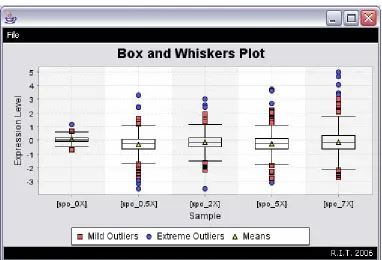
Figure 22: DiffExpress - Box and Whiskers Plot
A box plot can be used to graphically represent the minimum value, maximum value,
lower quartile, upper quartile and median of a set of data.9 This graph can also be used to
calculate the mean of the data and for the identification of outliers (unusual observations).
Placing two or more categorical box plots (one for each condition) side by side on the same
graph (Figure 22) can assist in comparing the datasets’ distributions and determining if there
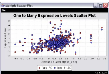
3.3.2.3 Scatter Plots
Figure 23: DiffExpress - Scatter Plot
Scatter plots (Figure 23) graphically display the spread of the data, illustrate the
relationship between two variables, and are helpful when determining if it is appropriate to
calculate the correlation coefficient or fit a regression curve. These graphs are also used for
easier identification of outliers in datasets. In cDNA microarrays, a common scatter plot
drawn is that of green versus red channel intensities.
The pattern in these types of graphs (scatter plots) is more apparent when there is a
plethora of data. If the data points come close to forming a straight line, then the higher the
correlation between the two variables. If the slope of the graph rises from left to right (a
while a slope falling from left to right (diagonal line from high y values to high x values)
represents a negative correlation.
A scatter plot may reveal some existing relationship between variables, but it does not
mean that one variable is causing a change in another variable. Another variable may be the
reason why the two variables seem related or their relationship may simply be coincidental.
3.3.2.4 Pearson Correlation Coefficient
When examining the relationship between variables the following questions can be asked:
1. Are two variables related in some way? (As one variable changes, does the other
variable also change in a linearly consistent way?)
2. What is the strength of the relationship?
The Pearson Correlation Coefficient (r) (Equation 5) is a number that describes the strength
and the direction of a relationship. The sign (+ or -) represents the direction (i.e. positive or
negative) while the magnitude corresponds to the strength of the correlation (i.e. weak or
strong correlation).
Even if there is a correlation, it does not signify that there is a causal relationship. A
significant correlation will only demonstrate that the two variables linearly vary together in a
certain direction (positively or negatively).
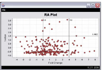
[image:52.612.107.494.188.453.2]3.3.2.5 RA Plot
Figure 24: DiffExpress - RA Plot
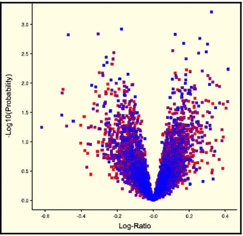
The RA Plot of DiffExpress is a modified version of the volcano plot (Figure 24).
Volcano plots (Figure 25) graphically display the relationship between the expression
change and statistical significance (using the t-test), thereby making it easier to detect
significant differentially expressed genes. The volcano plot’s horizontal axis(x) represents a
measure of expression change (usually the log ratio) between the two groups while its vertical
from the t-test, which is a parametric test used to assess whether there is a statistically
significant difference between the means of two groups.10
The RA plot’s horizontal axis also represents a measure of expression change (usually
the log ratio) between the two groups, but unlike the volcano plot, its vertical axis represents
the t-value calculated from the t-test, not a p-value.
Figure 25: Volcano Plot
(http://genstat.co.uk/doc/8doc/html/marray/VolcanoPlot.htm)
Region Expression Change Statistical Significance Upper Left and Right Greater than k-fold difference Statistically Significant
Upper Middle Less than k-fold difference Statistically Significant
Lower Left and Right Greater than k-fold difference Not Statistically Significant
[image:53.612.108.345.239.469.2]Lower Middle Less than k-fold difference Not Statistically Significant
Genes/ Spot ids with statistically significant values based on the t-test and with a large
log ratio will be identified as possibly being differentially expressed. The statistically
significant values of interest are those that are in the upper left and right regions of the plot
(Table 7).
Paired t-test
The paired t-test is used to compare the means between two of the same or related
samples, and is commonly used when a subject is measured before and after some
experiment.11 For example, it may be interesting to test the significance of the differences of
measurements of the pulse rate or blood pressure of a group of subjects before and after
receiving a certain drug at different times during the day.
Unpaired t-test
The unpaired t-test, also known as the independent group t-test, is used to compare
the means of two independent groups.11 An example is the blood pressure between a group of
patients who have received a certain medication and another group or patients who have
received a placebo. Unlike a paired test which uses non-random samples, this test should be
used when a replicate is randomly chosen from a population.
Expression Change
To calculate the expression change of the RA plot for both paired and unpaired
groups, the log is taken of the mean of the y group divided by the mean of the x group
⎟
⎠
⎞
⎜
⎝
⎛
=
x
y
change
Expression
log
2 (6)3.3.3 Expression Profile
When the candidate differentially expressed genes are identified, DiffExpress allows
the user to generate an expression profile (an example is shown in Figure 26). Basically, this
profile is a list of the candidate genes or proteins and the expression levels of the
corresponding samples (expression changes when dealing with cDNA input data). After the
profile has been created, the data can be analyzed and scanned for patterns (up regulated or
down regulated genes) or unusual values.
4 Implementation
4.1 Java
Java was used to implement DiffExpress because it is fast, robust and
platform-independent (the same program can be executed on multiple operating systems). The
complete Javadoc documentation for this tool can be referenced from the folder containing
the DiffExpress program files.
4.2 JFreeChart
JFreeChart (used for the creation of all DiffExpress graphs) is a chart library founded
by David Gilbert and written entirely in Java. JFreeChart supports the drawing of various
graphs such as histograms, pie charts, bar charts and scatter plots, just to name a few. Details
of this library can be found at: http://www.jfree.org/jfreechart/index.html.
4.3 Packages
A Java package is comprised of a group of related classes and interfaces. Five of the
main packages in DiffExpress (Basics, Comparators, Datasets, Frames and Graphs), are
described below.
4.3.1 Basics
The Basics package comprises of the majority of the classes designed to perform calculations
in DiffExpress.
Class Description
FoldChange Calculates the intensity ratio, log2 ratio or fold change for the input
Outliers Performs all calculations associated with identifying outliers using Tukey’s method. For each dataset, this class calculates the mean, median, interquartile range, maximum value, minimum value and cutoffs for mild and extreme outliers.
PCC Calculates the pearson correlation coefficient between two samples.
ReadInData Enters the input data into DiffExpress.
RAPlot Calculates t-values and fold changes for the RA plot.
4.3.2 Comparators
This package consists of all the comparators.
Class Description BWDatasetComparator Comparator to sort the box and whisker’s dataset.
FourthVarIDComparator Comparator to sort the samples by the second condition.
SampleIDComparator Comparator to sort the samples by the sample id.
ThirdVarIDComparator Comparator to sort the samples by the first condition.
4.3.3 Datasets
This package comprises of all the dataset classes and basic classes.
Class Description
BWDataset Box and whiskers dataset object.
CustomXYDataset Creates XY datasets for the RA Plot, Outliers Plot, Expression Levels
Plot and Expression Change Plot.
Samples Samples object.
Settings Settings object.
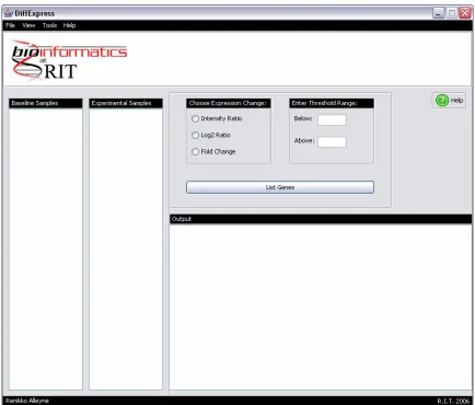
4.3.4 Frames
This package contains the user interfaces for DiffExpress.
Class Description
ExpressionFrame Main application window. The user can select samples,
choose the type of expression change, enter the threshold range, and obtain a list of the candidate differentially expressed genes or proteins. (Figure 27)
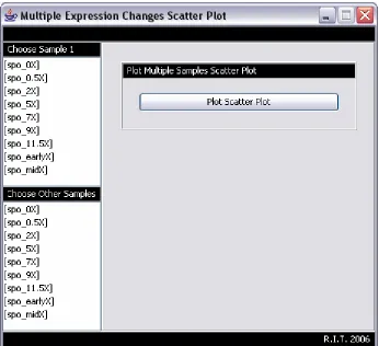
cDNAScatterPlotFrame Options window for cDNA expression changes scatter
plot. The user selects a sample from the “Choose Sample 1” list, and selects one or more samples from the “Choose Other Samples” list. (Figure 28)
ExpressionChangeScatterPlotFrame Options window for oligonucleotide and 2D gels expression change scatter plots. The user can select a baseline sample and two experimental samples. They can draw intensity ratio, log2 ratio or fold change
scatter plots, and calculate the pearson correlation coefficient for the samples selected. (Figure 29)
ExpressionLevelsBasicPlotFrame Options window for expression levels basic plot. The user can select one or more samples to plot on the same graph. (Figure 30)
GeneProfileTableFrame Window for the gene expression profile of candidate genes window.
GraphFrame Window for all individual graphs (i.e. the user has not
opted for “Multiple Plots in a Single Window”).
OutliersFrame Outliers and Box and Whiskers plot options window.
The user can select one or more samples and select a plot to be drawn. From the “Display Outlier Information” tab they may also display the values for the non-outliers, outliers and statistical values. (Figure 31 and Figure 32)
PCCFrame Pearson correlation coefficient options window. The
user can select two samples and calculate their pearson correlation coefficient. (Figure 33)
RAErrorFrame RA plot error dialog. If the two group sizes for a paired
t-test are not equal, this window pops up. (Figure 34)
RAPlotFrame RA plot options window. The user can select the
Figure 30: DiffExpress - Expression Levels Basic Plot Options Window
[image:62.612.109.431.69.274.2]Figure 31: DiffExpress - Outliers and Box & Whiskers Plot: Plot Graphs
Figure 33: DiffExpress - Pearson Correlation Coefficient Options Window
4.3.5 Graphs
This package contains classes that plot the various graphs that DiffExpress supports.
Class Description
MyBoxPlot Draws the box and whiskers plot for any type of input data.
PlotBasicGraph Draws the expression levels basic plot for oligonucleotide
and 2D gel data, i.e. Expression level vs. gene.
PlotGraph Draws the expression change basic plot for any type of input
data, i.e. Expression change vs. gene.
PlotOutlier Draws the outliers plot for any type of input data.
PlotRAPlot Draws the RA plot for oligonucleotide or 2D gel data.
5 PROBLEMS FACED
5.1 Missing Values
Missing values in the expression data matrix proved to be a problem initially. There
are a variety of ways to account for missing values, but in the end it was decided that the user
should do any preprocessing regarding missing values before the data file is loaded into the
tool. This way allows the user some flexibility on how to deal with their missing values,
rather than having the tool use a default that may not be suitable to their needs.
5.2 Infinity Values
Some infinity values appeared when the calculation of the expression change was
performed. Infinity values are problematic when creating the graphs because they are out of
range of the particular axis with which they belong. Initially the infinity values were
converted to zeroes, but this led to inaccurate graphs. In the end it was easier to exclude the
6 FUTURE WORK
6.1 Preprocessing
Preprocessing is used to make data suitable for analysis purposes. DiffExpress
performs no preprocessing; instead the user has to enter data that has already been
preprocessed. Some suggestions for preprocessing methods that can be added to DiffExpress
are as follows:
1. Imputation: for missing values.
2. Normalization: to ensure that differences in intensities are because of differential
expression and not errors made when the experiment was carried out.
3. Averaging replicates.
4. Filtering bad data.
6.2 Volcano Plot Implementation
The current version of DiffExpress implements the RA Plot – a modified version of
the Volcano Plot. An improvement to DiffExpress would be to implement an actual Volcano
Plot which uses the p-value.
6.3 Clustering
Another addition to DiffExpress could be that of clustering. Clustering of data is
advantageous because it helps to group genes according to patterns in their expression. Some
k-6.4 Identification of Differentially Expressed Genes
Implementing more methods for finding differentially expressed genes is also an
excellent addition. Chen’s single slide method, Sapir and Churchill’s single slide method, and
REFERENCES
1. University of Utah.; Profiling Technique: Protein Expression Analysis,
http://gslc.genetics.utah.edu/units/pharma/phprotan/ (accessed November 13th 2005).
2. Kimball, J.; “Gene Translation: RNA Æ Protein.” Biology,
http://users.rcn.com/jkimball.ma.ultranet/BiologyPages/T/Translation.html (accessed
November 13th 2005).
3. University of Utah.; Profiling Technique: Microarray Analysis,
http://gslc.genetics.utah.edu/units/pharma/phmicroarray/ (accessed November 13th 2005).
4. National Center for Biotechnology Information. Microarrays: Chipping Away At the Mysteries of Science and Medicine.
http://www.ncbi.nlm.nih.gov/About/primer/microarrays.html (accessed April 24th 2006).
5. Borman, S.; “Proteomics: Taking Over Where Genomics Leaves Off.” Science/Technology. 78: 31-37 (2000).
6. Coe, B.; Antler, C. Spot Your Genes – An Overview of the Microarray.
http://www.bioteach.ubc.ca/MolecularBiology/microarray/ (accessed April 25th 2006).
7. Bonetta, L. The Basics of DNA Microarrays.
http://www.hhmi.org/biointeractive/genomics/microarray.html (accessed April 25th
2006).
8. Saeed, A.; Analyzing Multiple Experiments with MeV,
http://www.jax.org/courses/archives/2004/MicroF04_Saeed_Presentation.pdf (accessed
November 1st 2005).
9. How to Draw a Boxplot. http://exploringdata.cqu.edu.au/box_draw.htm (accessed April 25th 2006).
10. Cui, X.; Churchill, G.; “Statistical Tests for Differential Expression in cDNA Microarray Experiments.” Genome Biology. 4:210 (2003).
DIFFEXPRESS USER GUIDE
1 GETTING STARTED
In order to begin using DiffExpress, double click the Threshold.jar file, or the following
command: java –jar Threshold.jar may be run from the command line or terminal window.
2 DIFFEXPRESS INTERFACE
[image:71.612.108.522.257.621.2]The interface (Figure A1) consists of a menu bar (Figure A2) and a work space (Figure A7).
2.1 Menu Bar
Figure A2: DiffExpress Menu Bar
[image:72.612.104.547.101.494.2]2.1.1 File
Figure A3: File Menu
Menu Item Description
File/ Open Input File Load a new expression matrix by opening a new file.
File/ Load Project Load an existing project.
File/ Save/ Save Output Save differentially expressed genes output.
File/ Save/ Save Project Save current settings.
File/ Close Project Close current project.
File/ Exit Exit DiffExpress.
2.1.2 View
Menu Item Description
View/ Graphs/ cDNA Graphs/ Expression Change Plot
Create cDNA expression change basic plot.
View/ Graphs/ cDNA Graphs/ Expression Change Scatter Plot
Create cDNA expression change scatter plot.
View/ Graphs/ Oligonucleotide or 2D Gel Graphs/ Basic Plots/ Expression Levels Plot
Create oligonucleotide or 2D gel expression levels basic plot.
View/ Graphs/ Oligonucleotide or 2D Gel Graphs/ Basic Plots/ Expression Change Scatter Plot
Create oligonucleotide or 2D gel expression change scatter plot.
View/ Graphs/ Oligonucleotide or 2D Gel Graphs/ Comparison Plots/ Expression Change Plot
Create oligonucleotide or 2D gel expression change basic plot.
View/ Graphs/ Oligonucleotide or 2D Gel Graphs/ Comparison Plots/ Expression Levels Scatter Plot
Create oligonucleotide or 2D gel expression levels scatter plot.
View/ Graphs/ RA Plot Create RA plot.
View/ Graphs/ Box and Whiskers Plot Create Outliers plot or Box and Whiskers plot.
View/ External File View an external text file.
View/ Gene Expression Profile View the gene expression profile of differentially expressed genes.
[image:73.612.94.549.69.460.2]2.1.3 Tools
Menu Item Description
Tools/ Options/ Sort Samples List Sort sample list by sample id, first condition, or second condition.
Tools/ Options/ Multiple Plots in a Single Window
Group related graphs in a single window.
Tools/ Data Information/ Basic Data Information
View basic information about the input data, such as number of genes or spot ids, number of samples, gene ids or spot ids, and sample ids.
Tools/ Data Information/ Advanced Data Information
Enables user to specify the type of input data loaded.
Tools/ Calculate PCC Calculate the Pearson correlation coefficient between
two selected samples.
[image:74.612.101.546.75.338.2]2.1.4 Help
Figure A6: Help Menu
Menu Item Description
2.2 Work Space
Figure A7: DiffExpress Workspace
(A) Samples Lists, (B) Expression change and Threshold Range options, (C) Output Window
The work space allows the user to select samples, choose an expression change, enter a
threshold range, and view the differentially expressed genes.
3 LOADING DATA
Expression data can be loaded either by opening a new input file (File/ Open Input File) or
loading an existing project (File/ Load Project). If a new input file is opened, the Advanced
Data Information Option Window will open (Figure A8). This option window allows the
user to specify the type of input data that has been loaded. This information may be entered
A
now or at a later time, but it must be entered before any analysis and viewing of graphs can
[image:76.612.110.412.132.538.2]be performed.
Figure A8: Advanced Data Information Option Window
If the user would like to change the advanced data information at anytime, they can do so by
performing the following from the menu bar: Tools/ Data/ Information/ Advanced Data
4 SAVING
4.1 Save Output
The information in the Output Window of the work space may be saved to a text file if
desired (File/ Save Output).
4.2 Save Project
To save the current settings perform the following from the menu bar: File/ Save Project.
These saved settings are the files used when loading existing projects.
4.3 Save Graphs
Graphs may be saved in jpeg format by using the File/ Save option on the respective graph’s
menu bar, or (on Windows systems) by right clicking on the graph and selecting the Save as
[image:77.612.112.497.406.664.2]option (Figure A9).
5 Viewing
5.1 View Graphs
DiffExpress provides basic plots, scatter plots, outliers plots, box and whiskers plots and RA
plots.
5.1.1 cDNA Data Graphs
Expression Change Plot
This is a plot of expression change versus genes for selected samples. Follow these steps to
create an expression change plot (Figure A10):
1. Select one or more samples from the Baseline Samples list.
2. Choose a type of expression change.
3. Enter in a threshold range.
[image:78.612.107.519.316.648.2]4. From the menu bar: View/ Graphs/ cDNA Graphs/ Expression Change Plot
Figure A10: Drawing cDNA Expression Change Plot
1 3
4
Expression Change Scatter Plot
This is a scatter plot of the expression change of one or more selected samples versus the
expression change of another sample. Follow these steps to create an expression change
scatter plot (Figure A11):
1. From the menu bar: View/ Graphs/ cDNA Graphs/ Expression Change Scatter Plot.
2. Select one sample from the Choose Sample 1 list.
3. Select one or more samples from the Choose Other Samples list.
4. Click the Plot Scatter Plot button.
1
3
[image:79.612.116.544.227.680.2]5.1.2 Oligonucleotide or 2D Gel Data Graphs
5.1.2.1 Basic Plots
Basic Plots do not require the user to make selections DiffExpress’ work space. They have
their own dialogs from which selections can be made.
Expression Levels Plot
This is a plot of expression levels versus genes for selected samples. Follow these steps to
create an expression levels plot (Figure A12):
1. From the menu bar: View/ Graphs/ Oligonucleotide or 2D Gel Graphs/ Basic Plots/
Expression Levels Plot.
2. Select one or more samples from the Samples List list.
[image:80.612.111.542.330.675.2]3. Click the Plot button.
Figure A12: Expression Levels Basic Plot Options Window
1
Expression Change Scatter Plot
This is a plot of the expression change between the selected baseline s