promoting access to White Rose research papers
White Rose Research Online [email protected]
Universities of Leeds, Sheffield and York
http://eprints.whiterose.ac.uk/
This is an author produced version of a paper published in Combinatorial Chemistry and High Throughput Screening
White Rose Research Online URL for this paper: http://eprints.whiterose.ac.uk/7690/
Published paper
Grouping Of Coefficients For The Calculation Of
Inter-Molecular Similarity And Dissimilarity
Using 2D Fragment Bit-strings
J. D. Holliday
1, C-Y. Hu
2and P. Willett
Krebs Institute for Biomolecular Research and Department of Information Studies,
University of Sheffield, Western Bank, Sheffield S10 2TN, UK
1 To whom all correspondence should be addressed: email [email protected] 2
ABSTRACT
This paper compares 22 different similarity coefficients when they are used for searching
databases of 2D fragment bit-strings. Experiments with the NCI AIDS and ID Alert
databases show that the coefficients fall into several well-marked clusters, in which the
members of a cluster will produce comparable rankings of a set of molecules. These clusters
provide a basis for selecting combinations of coefficients for use in data fusion experiments.
The results of these experiments provide a simple way of increasing the effectiveness of
INTRODUCTION
Methods for calculating the similarities (or dissimilarities) between pairs, or larger groups, of
molecules play an important role in many aspects of chemoinformatics, such as similarity
searching [1], property prediction [2], synthesis design [3], virtual screening [4] and
molecular diversity analysis [5], inter alia. For example, measures of dissimilarity lie at the
heart of many of the algorithms that are used to select libraries of compounds for synthesis
and testing that are as structurally diverse as possible. Again, similarity searching involves
calculating a measure of structural similarity between a target structure and each of the
structures in a database; if the target structure is bioactive, e.g., a weak lead in a drug
discovery programme, then inspection of the nearest neighbours resulting from the similarity
search can suggest new molecules for biological testing.
The effectiveness of such procedures will be affected by the measure that is used to quantify
the degree of similarity or dissimilarity between pairs of structures. There are two principal
components to a similarity measure: the representation that is used to characterise the
molecules that are to be compared, this often being a set of descriptors such as 2D fragment
substructures or sets of calculated physicochemical properties [6,7]; and the similarity
coefficient that is used to quantify the degree of resemblance between two such
representations. The representation may need some form of pre-processing before the
similarity calculation (e.g., descriptor values may need to be weighted or standardised prior
to the similarity calculations), thus introducing a third component in such cases. In this
paper, we focus on similarity coefficients, in particular their use for measuring similarities
between pairs of 2D fragment bit-strings (or fingerprints). These representations provide a
very simple encoding of molecular structure but have been found to yield a surprisingly high
Many different types of similarity coefficient have been described in the literature but most
of them can be grouped into three broad classes: distance coefficients, association
coefficients and correlation coefficients. Distance coefficients quantify the degree of
difference between two objects and have been extensively used in many applications of
multivariate statistics (especially where integer-valued or real-valued variables are
employed), probably due to the simple geometric interpretation that is attached to many of
them (e.g., the Euclidean distance). With a distance coefficient, the greater the degree of
similarity between two objects the smaller the value of the coefficient (and vice versa).
Association coefficients, conversely, are most commonly used with binary data (i.e.,
variables denoting the presence or absence of descriptors in an object) and are often
normalised to lie within the range of zero (no similarity at all) and unity (identical sets of
descriptors). That said, association coefficients can be used with non-binary data, in which
case other ranges of values may apply (e.g., the lowerbound of the well-known Tanimoto
coefficient is –1/3 when used with such data [1]). Finally, correlation coefficients measure
the degree of correlation between the sets of values characterising each of a pair of objects
(rather than their more conventional use in multivariate analyses to probe the relationships
between pairs of variables). There have been several studies comparing the merits of
different chemical similarity measures (see, e.g., [11-13]). It has been found that the
Tanimoto coefficient provides a generally effective approach to molecular property
prediction and similarity searching, and this coefficient is now widely used for measuring the
similarity between pairs of 2D bit-strings (despite some limitations that have recently become
apparent [14-16]).
In this paper, we report a comparison of some 22 different similarity coefficients (16
association coefficients, 5 correlation coefficients and 1 distance coefficient) when used with
2D fragment bit-string data, with the aim of identifying some subset of these that exemplify
searches using each of the coefficients in turn, clustered them on the basis of the search
outputs, and then evaluated the search effectiveness of various combinations of the individual
coefficients.
EXPERIMENTAL DETAILS
Assume that the bit-strings XP and XQ denote two molecules P and Q, respectively, and that
each of these strings contains a total of n bit positions. Assume further that b and c of these n
bits are set to one only in XP and only in XQ, respectively, that a of these n bits are set to one
in both XP and XQ, and that d of these n bits are not set in either XP and XQ (so that n = a +
b + c + d). Then the various coefficients used here are as shown in Fig. (1), with the first 16
entries being association coefficients, the next five entries being correlation coefficients and
the last being a distance coefficient. These coefficients are drawn from the extensive review
by Ellis et al. [17], who also include several other distance coefficients. However, all but one
of these (the Bray-Curtis distance) are completely monotonic, i.e., will result in identical
rankings of a set of molecules in response to a query, and we have hence used just one of
them, the mean Manhattan Distance, in our experiments1. The remaining distance
coefficient, the Bray-Curtis, has also been omitted as it proved to be the complement of the
Dice Coefficient (coefficient-2 in Fig. (1)). The reader is referred to the review by Ellis et al.
for a detailed discussion of the origins of the various coefficients that we have tested here
[17].
The principal dataset used in our experiments was the 1999 version of the National Cancer
Institute’s AIDS database [18], which contains compounds that have been tested for anti-HIV
activity. Salts and duplicate structures were removed from this file to give a total of 37,124
compounds, 294 of which have been confirmed as showing strong activity. These molecules
were represented by their UNITY 2D fragment bit-strings [19], hashed fingerprint
1
representations which encode the 2D structural features present in the molecule. These
features include fragment-based sequences of length two to six, five- and six-membered ring
systems, and counts of non-carbon atoms. The bit-strings for all of the compounds were used
in all of the experiments discussed below. 60 of the strongly active molecules were chosen
from the file to act as the target structures for database searching.
CLUSTERING OF RANKINGS
A similarity search of the AIDS database was carried out using each of the 22 similarity
measures shown in Fig. (1). The results of each search were ranked in decreasing order of
the calculated similarity coefficient (or the complement in the case of the distance
coefficient). The rankings for two searches can be compared by counting the number of
compounds in common in the top t structures, (where t has been chosen as 50, 100, 200 and
400 for this experiment); then the dissimilarity value Dij between searches using coefficients i
and j is defined to be
t
c
D
ij=
1
−
ij ,where cijis the number of common structures in the top t ranking positions. It is hence
possible to generate a t×t dissimilarity matrix for each target structure, illustrating the
relationships between pairs of similarity coefficients for that target at the chosen value of t.
Three different agglomerative hierarchical clustering methods (single linkage, complete
linkage and group-average) were then applied to each such dissimilarity matrix; the
clustering of similarity coefficients to identify inter-coefficient relationships was first
suggested by Hubaleck in the context of fungal species extracted from birds and bird nests
[20]. The dendrograms obtained here, using the first target structure and with t=50, are
After clustering, Mojena’s stopping rule [21] was used to determine a stopping level at which
to partition each of the resulting dendrograms into appropriate groups. Here, a hierarchy on
m objects is partitioned at that level for which
σ
µ
α
j+1>
+
k
where α0, α1….αm-1 are the dissimilarity levels at which each successive agglomeration takes
place, these corresponding to stages with m, m-1….1 clusters. The terms µ and σ are the
mean and unbiased standard deviation, respectively, of the α values, and k is a constant
(which we set to 1.25 as suggested by Milligan and Cooper [22]).
By using Mojena’s stopping rule, the dendrograms of Figs. (2-4) are all partitioned to give
(the same) three groups. These are (the numbers in the groups correspond to the coefficients
in Fig. (1)):
Group A : {1 2 4 5 11 12 15 17 20 21}
Group B : {3 13 16 18 19}
Group C : {6 7 8 9 10 14 22}
The same procedure was carried out for all classifications (60 different target structures and
three different clustering methods for each target) and we then combined the resulting 180
sets of groupings to identify groups of coefficients that are always clustered together. This
overall grouping contained a total of 11 groups as follows:
Group A : {3}
Group B : {11}
Group C : {14}
Group D : {16}
Group E : {18}
Group F : {21}
Group H : {6 7 8 9 10 22}
Group I : {12 15}
Group J : {13 19}
Group K : {17 20}
Thus, for example, coefficients 1, 2, 4 and 5 clustered together in all 180 tests, as did 6, 7, 8,
9, 10 and 22, etc. The reader should note that the presence of several coefficients in a group
does not imply that all of the coefficients are strictly monotonic; however, it does mean that
the sets of nearest neighbour compounds resulting from their use are very similar, and it is
these sets, rather than the precise rankings, that are normally required in database searching
applications
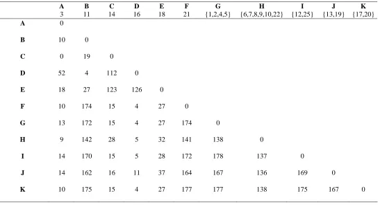
Having identified the groups of closely related coefficients, we can then assess the
relationships between these groups. These are illustrated in Table 1, which contains the
number of times that each of the 11 groups above clustered with one of the other 10 groups
over the whole set of 180 classifications. It will be seen that there are some very strong
relationships between the groups, e.g., Groups G and I (containing coefficients {1,2,4,5} and
{12,15}, respectively) clustered together in no less than 178 of the 180 tests. If we were to
use 170 co-occurrences, then these two groups would be joined by Groups B, F and K to give
the grouping {1,2,4,5,11,12,15,17,20,21}. Thus far, we have considered only the groupings
obtained with t=50, but very similar results are obtained if t is set to 100, 200 or 400, rather
than 50 as in Table 1. In fact, although there are 11 groups using the criteria discussed
above, the Mojena stopping rule normally identified just three or four groups of coefficients
in the great majority of the experiments that were carried out, whatever the target structure,
clustering method or value of t: one consisting mainly of coefficients from the set
{1,2,4,5,11,12,15,17,20,21}; one consisting mainly of coefficients from the set
{6,7,8,9,10,22}; and one consisting of the others, although coefficient 3 was often found on
To ensure that these results were not determined by the specific characteristics of the AIDS
database and of the target structures that were used, a comparable series of experiments was
carried out using 11607 structures for which biological activities have been reported in the
literature and which were entered into the IDAlert database during 1992-96 [23]. 60
molecules were again selected at random from this file and used as target structures for
similarity searching. The search rankings were analysed as described previously and yielded
groupings very similar to those obtained with the AIDS data. For example, using a threshold
of 170 with t=50, the largest group contained coefficients {1,2,4,5,12,15,17,20}, i.e.,
identical to that obtained with the AIDS dataset with the exception of coefficients 11 and 21,
both which here were in clusters on their own. This similarity of behaviour was observed for
searches using all four values of t (50, 100, 200 and 400).
It hence seems reasonable to conclude that there are groups of coefficients that tend to
produce analogous rankings when used for similarity searching in chemical databases. This
conclusion is hardly surprising when one considers the actual formulae in Fig. (1). For
example, we have noted that coefficients 6-10 occur together, and they all involve the term
a+d in the numerator of their defining expression; coefficient 22 (mean Hamming) also
co-occurs and subsequent inspection of its formula revealed that it is actually the complement of
coefficient 6 (Simple Match), as the term b+c in the Hamming numerator 22 is simply n
-(a+d). At the same time, there are coefficients that are markedly different from each other,
with the sets of top-ranked nearest neighbours having less than 5% of the molecules in
common. These differences are demonstrated in Table 1; we have already noted that
coefficient 3 is a frequent outlier, but coefficients 14, 16 and 18 also have notably fewer
co-occurrences (except with each other) than the other coefficients considered here.
An inspection of the literature on chemical similarity and dissimilarity reveals that while
there are many different similarity measures, most published studies have considered the use
of only a single measure. Even where this is not the case, multiple measures have typically
been employed only as the input to a comparative study that seeks to identify the “best”
measure, using some quantitative performance criterion. Such comparisons are limited in
that they assume, normally implicitly, that there is some specific type of structural feature,
weighting scheme or whatever that is uniquely well suited to describing the type(s) of
biological activity that are being sought for in a similarity search. The assumption cannot be
expected to be generally valid, given the multi-faceted nature of biological activities, and
there has thus recently been interest in the use of data fusion or consensus scoring methods
[24-27]. For example, Charifson et al. have discussed combining rankings based on different
scoring functions for docking searches [26], an idea that is embodied in the CSCORE
software package [19]. Such combined rankings generally give better results than use of an
individual scoring function or similarity measure, and small-scale experiments suggest that
the more rankings that are combined, the better the final results [27]. However, if many
different similarity measures are available, it may be too time-consuming to use all of them,
in which case it seems appropriate to ensure that as diverse a range of types of measure are
employed (in much the same way as one focuses on structural diversity when selecting
database subsets for biological testing). Here, we use the results of our clustering
experiments to provide a rational basis for selecting similarity coefficients for data fusion.
We took as our starting point the groups of coefficients identified previously, and then chose
one coefficient from each group as representative of the different types of similarity measure:
in many of the groups, of course, there was only a single coefficient to choose. The
coefficients chosen from groups A-K were as follows: 3 (Russell/Rao), 11
(Simple Match), 12 (Ochiai/Cosine), 13 (Kulczynski(2)) and 20 (Stiles), respectively. A set
of 20 active molecules was then randomly chosen from the AIDS database and each of these
was used as the target structure for a similarity search of the database, using each of the
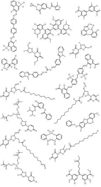
chosen coefficients in turn. These target structures are shown in Figure (5) to illustrate the
range of structural types considered in the searches.
We have already noted that most of the classifications suggested the presence of three groups
of coefficients, and fusion was hence carried out for each target structure by selecting the
rankings for three coefficients at a time. These rankings were merged by summing the
rank-positions for each compound to give a score that formed the basis for a new, final ranking
(this is the SUM fusion rule that was found to be the most effective in the study of Ginn et al.
[27]). Each ranking, whether from one of the 11 original individual coefficients or from one
of the 165 (3C11) combinations of coefficients, was then inspected to identify the number of
active molecules in the top 400 positions; this number was taken as the effectiveness of that
search, and hence of the effectiveness of the combination of coefficients, or the individual
coefficient, that was used in the search.
For each target structure, the combinations were sorted into decreasing order of the number
of actives retrieved and assigned an ordinal value from 1 (best ranking) down to 165 (worst
ranking); combinations with equal performance were assigned the mean ordinal value (i.e., if
the third, fourth and fifth best combinations all retrieved the same number of actives then
they are all assigned 4). The overall performance of each combination was then determined
by the sum of ordinal values across all 20 target structures, with the results in Table 2. The
upper part of this table contains the 10 best combinations, and the bottom part the 10 worst
combinations. If all of the combinations performed at the same level, then the summed value
would be 1660, i.e., the median of 1,2,3….164, 165, multiplied by 20 (the number of
effectiveness that can arise as the result of a good, or a bad, choice of coefficients for
carrying out data fusion. The table also contains the median numbers of actives retrieved
when averaged over the 20 searches, this again demonstrating clearly the substantial
performance differences that exist.
The top row of Table 2 represents the best single combination (on the basis of our chosen
measure of search effectiveness) and consists of the following three coefficients: the
Russell/Rao coefficient; the Simple Match coefficient; and the Stiles coefficient. Other
coefficients figuring prominently are Jaccard/Tanimoto and Kulczynski(2). It is worth
mentioning the fifth-ranked combination (Jaccard/Tanimoto, Russell/Rao and Simple Match)
as Dixon and Koehler have recently recommended the combination of Tanimoto and
Hamming (which we have seen is the complement of the Simple Match) for similarity
searching [16]. The worst single combination involves the Forbes coefficient, the Dennis
coefficient and the Simple Match coefficient, and all three of these figure prominently in the
bottom part of Table 2; Dennis indeed occurs in every one of them. It is surprising to see
Simple Match appearing so frequently here, given that it also figured prominently at the top
of the ranking. In fact, an analysis of all of the combinations involving this coefficient shows
that it appears in combinations that are spread throughout the ranked list of 165 combinations
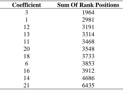
for each query, as we now demonstrate. Each individual coefficient, c, will occur in 45
different combinations with pairs of other coefficients; then the sum of the positions in the
ranked list for each of these 45 combinations will give an overall figure-of-merit for
coefficient c. These figures are shown in Table 3, from which we see that the best individual
coefficients (as manifested by their behaviour in the data fusion experiments) are
Russell/Rao, Jaccard/Tanimoto and then Ochai/Cosine, while the worst are Dennis (which
occurred in all of the 45 lowest ranked combinations), Forbes and then Simpson. The
frequent high and low appearances in Table 2 of Simple Match means that it occurs around
Previous studies of data fusion have suggested that appropriately combined rankings can be
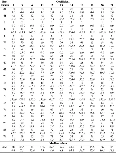
consistently superior to individual rankings, and this is certainly the case here. Table 4 lists
numbers of actives retrieved in each of the 20 searches for the 11 individual coefficients and
for the best three-way combination (i.e., Russell/Rao, Simple Match and Stiles). Each
element of the main body of the table also contains an enrichment factor. Assume that an
individual coefficient retrieves Ni actives, and the best three-way combination Nc actives, in
the top 400 rank positions. Then the enrichment is defined to be
i i c
N
N
N
−
100
The median values for numbers of actives retrieved and for the enrichment are listed at the
bottom of the table, where it will be seen that our best 3-coefficient combination is superior,
when averaged over the 20 searches, to all of the individual coefficients (in that the median
number of actives is greater than the numbers for the individual rankings, and in that all of
the enrichment factors are positive).
The focus of this section of the paper is the performance of the fused similarity coefficients,
but the median values in Table 4 enable one to compare the individual coefficients. If one
takes the numbers of actives retrieved, then the order is
1>11=12>13>20=21>18>6>3>16>14,
while for the enrichments the order is
13>1=12>3>11>20>21>6>18>16>14.
There is a fair degree of commonality with the ranking of the fused combinations discussed
above, albeit with some obvious discrepancies - specifically coefficient 3 (Russell/Rao) in the
actives retrieved and 21 (Dennis) in both actives retrieved and enrichment - when compared
with the combination rankings in Table 3. In general, then, if an individual coefficient
other effective coefficients; in a similar vein, poorly performing individual coefficients are
not expected to do well when combined with other poorly performing coefficients.
The clustering experiments suggested the existence of three groups of coefficients, and hence
the use of 3-way fusions in the experiments thus far. To confirm the optimality of this choice,
a further study was carried out in which all possible combinations of any number of
coefficients were investigated. The same method of fusion, the merging of rank-positions,
was used as for the 3C11 combinations, but this time we chose all nC11 combinations for values
of n from 2 to 11. The number of combinations for each value of n is shown in the second
column of Table 5. We used the same twenty actives as targets and merged the respective
rankings. Performance was measured in two ways: firstly, using the sum of ordinal
performance values as in the previous study; and, secondly, using the number of actives in
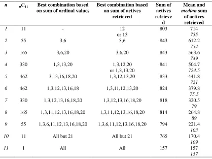
the top 400 rank positions summed across all 20 searches. The best combinations based on
these two performance measures for all values of n are shown in Table 5. This table also
includes values for the performance of the single coefficients (i.e., n=1) and, for each value
of n, indicates the sum of actives retrieved by the best combination and the mean and median
values for the sum of actives across all combinations. It will be seen that the best
combination is either 3 (Russell/Rao) and 6 (SimpleMatch) or 3, 6 and 20 (Stiles), i.e., the
best 3-way combination used previously. Both of these combinations retrieve the same
number of actives (843) and are a considerable improvement on the performance of the best
single coefficient (803 actives).
The median number of actives retrieved appears to fall considerably for combinations of
greater than six coefficients, reflecting the increasing influence of the poorly-performing
coefficients such as 21 (Dennis). The value for the sum of actives for the best combination
remains high for nearly all values of n, while the mean decreases steadily. When compared to
comparably well, and most combinations taken from this set (which appears to include
Russell/Rao, SimpleMatch, Stiles, Jaccard/Tanimoto, Ochiai/Cosine, Baroni-Urbani/Buser,
and Kulcynski(2)), should give an acceptable level of performance..
CONCLUSIONS
In this paper we have compared a range of similarity coefficients when they are used for
similarity and dissimilarity searching in databases of chemical compounds represented by 2D
fragment bit-strings. Our experiments with the NCI AIDS and IDAlert databases
demonstrate clearly that the coefficients fall into several well-marked clusters, in which the
members of a cluster will produce comparable sets of nearest neighbours in similarity
searches for a given target compound. We have then used these clusters as the basis for a
data fusion study in which we have combined the results of similarity searches based on three
different coefficients to produce new, fused rankings. These fused rankings are generally
more effective, in terms of retrieving bioactive molecules, than rankings based on just a
single coefficient, if an appropriate combination of coefficients is chosen for the fusion.
This finding provides a simple way of enhancing the performance of existing systems for
fragment-based similarity searching. Current systems compare the bit-string for a target
structure with the bit-strings of each of the molecules in a database, using the common and
non-common bits in each such comparison to calculate a value for (typically) the Tanimoto
coefficient. Our results suggest that if these common bits are additionally used to calculate
the values of other coefficients, then the resulting ranking will contain a larger number of
high-ranked active compounds than if just the Tanimoto is used. These additional coefficient
values can be calculated at negligible computational cost (since the bit-string comparisons
advocated here hence results in an increase in search effectiveness with only a very slight
decrease in search efficiency.
Clearly this work could be considerably extended, for example by using other types of 2D
fragment bit-string, by varying the number of coefficients involved in each combination
ranking, and by using datasets for which quantitative, rather than qualitative, bioactivity data
are available. Summarising the results we have obtained thus far, our experiments certainly
support the continued popularity of the Jaccard/Tanimoto coefficient for chemoinformatic
applications; in addition, researchers might also usefully consider, either alone or in
combination, the Russell/Rao, Baroni-Urbani/Buser, SimpleMatch, Stiles, Ochiai/Cosine, and
Kulczynski(2) coefficients.
The final point we wish to make is that our findings are specific to 2D fragment bit-strings;
and are not necessarily applicable to other types of representation. For example, the HQSAR
system [19] uses a representation that involves frequencies of occurrence of individual
fragments, rather than just their presence or absence. Other descriptors result in real-valued
representations, such as the sets of topological indices produced by MOLCONN-Z [28] or the
field values produced by 3D descriptors such as COMFA [19]. Such molecular descriptors
may require the use of standardisation and are also hospitable to a larger range of similarity
coefficients than used here (where many of the coefficients that one might consider are
rendered completely monotonic by the use of binary representations). The use of data fusion
with such descriptors provides another obvious area for future experimentation.
ACKNOWLEDGEMENTS
We thank the KC Wong Education Foundation for funding, Tripos Inc. for software support
Biomolecular Research is a designated biomolecular sciences centre of the Biotechnology
and Biological Sciences Research Council.
REFERENCES
1. Willett, P.; Barnard, J.M.; Downs, G.M. J. Chem. Inf.Comput. Sci., 1998, 38, 983.
2. Brown, R.D.; Martin, Y.C. J. Chem. Inf. Comput. Sci. 1996, 36, 572.
3. Wipke, W.T.; Rogers, D. J. Chem. Inf.Comput. Sci., 1984, 24, 71.
4. Bohm, H.-J. ; Schneider, G., Eds. Virtual Screening for Bioactive Molecules,
Wiley-VCH: Weinheim, in the press.
5. Dean, P.M.; Lewis, R.A., Eds. MolecularDiversity in Drug Design, Kluwer: Amsterdam,
1999.
6. Brown, R.D. Perspect. Drug Disc. Design, 1997, 7/8, 31.
7. Patterson, D.E., Cramer, R.D., Ferguson, A.M., Clark, R.D. and Weinberger, L.E.
Neighbourhood behaviour: a useful concept for validation of “molecular diversity”
descriptors. Journal of Medicinal Chemistry, 1996, 39, 3049-3059.
8. Willett, P. Similarity and Clustering in Chemical Information Systems, Research Studies
Press: Letchworth, 1987.
9. Potter, T.; Matter, H. J. Med. Chem., 1998, 41, 478.
10. Bayada, D.M.; Hamersma, H.; van Geerestein, V.J. J Chem. Inf. Comput. Sci., 1999, 39,
1.
11. Adamson, G.W.; Bush, J.A. J. Chem. Inf. Comput. Sci., 1975, 15, 55.
12. Willett, P.; Winterman, V. Quant. Struct.-Activ. Relat., 1986, 5, 18.
13. Cheng, C.; Maggiora, G.M.; Lajiness, M.S.; Johnson, M.A. J. Chem. Inf. Comput. Sci.,
1996, 36, 909.
14. Flower, D. J. Chem. Inf. Comput. Sci., 1998, 38, 379.
16. Dixon, S.L.; Koehler, R.T. J. Med. Chem., 1999, 42, 2887.
17. Ellis, D.; Furner-Hines, J.; Willett, P. Perspect. Inf. Manag., 1994, 3, 128.
18. The AIDS database is available from the NCI/NIH Developmental Therapeutics
Programme at URL http://dtp.nci.nih.gov/
19. The UNITY, COMFA, HQSAR and CSCORE software packages are available from
Tripos Inc. at URL http://www.tripos.com
20. Hubalek, Z. Biol. Rev., 1982, 57, 669.
21. Mojena R. Computer J. , 1977, 20, 359-363
22. Milligan G.W.; Cooper M.C. Psychometrika, 1985, 50(2), 159-179
23. The IDAlert database is available from Current Drugs Limited at URL
http://www.current-drugs.com/
24. Kearsley, S.K.; Sallamack, S.; Fluder, E.M.; Andose, J.D.; Mosley, R.T.; Sheridan, R.P.
J. Chem. Inf. Comput. Sci., 1996, 36, 118.
25. Ginn, C.M.R.; Turner, D.B.; Willett, P.; Ferguson, A.M.; Heritage, T.W. J. Chem. Inf.
Comput. Sci., 1997, 37, 23.
26. Charifson, P.S.; Corkery, J.J.; Murcko, M.A.; Walters, W.P. J. Med. Chem., 1999, 42,
5100.
27. Ginn, C.M.R.; Willett, P.; Bradshaw, J. Perspect. Drug Discov. Design, in the press.
1. Jaccard/Tanimoto
c
b
a
a
+
+
2. Dicec
b
a
a
+
+
2
2
3. Russell/Raon
a
4. Sokal/Sneath(1)c
b
a
a
2
2
+
+
5. Kulczynski(1)c
b
a
+
6. Simple Matching
n
d
a
+
7. Hamannn
c
b
d
a
+
−
−
8. Sokal/Sneath(2)
n
d
a
d
a
+
+
+
2
2
9. Rogers/Tanimoton
c
b
d
a
+
+
+
10. Sokal/Sneath(3)c
b
d
a
+
+
11. Baroni-Urbani/Buserc
b
a
ad
a
ad
+
+
+
+
12. Ochiai/Cosine)
)(
(
a
b
a
c
a
+
+
13. Kulczynski(2))
)(
(
)
2
(
2
c
a
b
a
c
b
a
a
+
+
+
+
14. Forbes)
)(
(
a
b
a
c
a
n
+
+
×
15. Fossum)
)(
(
2
1
2c
a
b
a
a
n
+
+
−
16. Simpson)
,
min(
a
b
a
c
a
+
+
17. Pearson)
)(
)(
)(
18. Yule
bc
ad
bc
ad
+
−
19. McConnaughey
)
)(
(
2
c
a
b
a
bc
a
+
+
−
20. Stiles
)
)(
)(
)(
(
2
log
2
10
d
c
d
b
c
a
b
a
n
bc
ad
n
+
+
+
+
−
−
21. Dennis
)
)(
(
a
b
a
c
n
bc
ad
+
+
−
22. Mean Manhattan
n
c
b
+
Figure 1. Association coefficients (1-16), correlation coefficients (17-21) and distance coefficient (22) used in the experiments.
Figure 2. Dendrogram for single linkage clustering of first target structure dissimilarity matrix;
Figure 4. Dendrogram for group average linkage clustering of first target structure dissimilarity matrix;
Figure 5. The 20 actives from Aids database used as target structures used for data fusion. S O O O O N N S O O O O N N O S N O O Cl N O O O O N O O O O O O S S O O N N S Cl F N N O O O O F O N N N N N N O N N N N N O F O F O O O O N N S O O O O O O N N S O O O O O Cl N S N N O O O N N N O O O N O O O O Cl N N N O O O N N N O O Cl O O O O O O Cl O O O Cl O O O O N N O O O O P O O O O O O O N O O S N O O O O N N O O O N N N O N N N O N N O N O F O P O O O O O O
O N N
A
3
B
11
C
14
D
16
E
18
F
21
G
{1,2,4,5}
H
{6,7,8,9,10,22}
I
{12,25}
J
{13,19}
K
{17,20}
A 0
B 10 0
C 0 19 0
D 52 4 112 0
E 18 27 123 126 0
F 10 174 15 4 27 0
G 13 172 15 4 27 174 0
H 9 142 28 5 32 141 138 0
I 14 170 15 5 28 172 178 137 0
J 14 162 16 11 37 164 167 136 169 0
[image:25.842.152.699.111.407.2]K 10 175 15 4 27 177 177 138 175 167 0
Combination Ordinal Value Median Actives
3,6,20 993.5 40.5
3,12,13 1032.5 37.5
1,3,13 1047.0 37.5
1,3,12 1054.0 37.5
1,3,6 1065.5 40.0
3,6,12 1082.0 40.0
3,6,11 1089.0 40.0
3,11,18 1093.0 37.0
3,6,13 1105.5 40.0
1,13,18 1108.0 37.5
11,18,21 3748.0 2.0
13,14,21 3756.0 1.0
6,11,21 3764.0 1.0
14,16,21 3854.0 1.0
6,20,21 3856.0 1.0
6,18,21 3881.5 1.0
6,16,21 3956.0 1.0
14,18,21 3964.5 1.0
14,20,21 3964.5 1.0
6,14,21 3977.5 1.0
Table 2: Best (top 10 rows) and worst (bottom 10 rows) combinations of coefficients for similarity searching in the AIDS database. The second column gives the sum of rank positions over the set of 20 target structures, and the third column the median number of actives retrieved when averaged over these 20 searches.
Coefficient Sum Of Rank Positions
3 1964
1 2981
12 3191
13 3314
11 3468
20 3548
18 3733
6 3853
16 3912
14 4686
[image:26.595.163.433.83.350.2]21 6435
[image:26.595.212.411.429.574.2]Coefficient Best
Fusion 1 3 6 11 12 13 14 16 18 20 21
34 33
3.0 34 0.0 34 0.0 33 3.0 33 3.0 33 3.0 28 21.4 34 0.0 34 0.0 33 3.0 33 3.0
41 42
-2.4 32 28.1 42 -2.4 42 -2.4 42 -2.4 42 -2.4 31 32.3 31 32.3 38 7.9 42 -2.4 42 -2.4
1 1
0.0 2 -50.0 1 0.0 1 0.0 1 0.0 1 0.0 1 0.0 1 0.0 1 0.0 1 0.0 1 0.0
8 7
14.3 12 -33.3 2 300.0 4 100.0 8 0.0 9 -11.1 2 300.0 12 -33.3 6 33.3 4 100.0 4 100.0
5 5
0.0 5 0.0 5 0.0 5 0.0 5 0.0 5 0.0 4 25.0 4 25.0 5 0.0 5 0.0 5 0.0
79 73
8.2 70 12.9 63 25.4 69 14.5 72 9.7 70 12.9 34 132.4 61 29.5 65 21.5 68 16.2 66 19.7
3 3
0.0 4 -25.0 3 0.0 3 0.0 3 0.0 3 0.0 3 0.0 3 0.0 3 0.0 3 0.0 3 0.0
73 68
7.4 70 4.3 61 19.7 66 10.6 68 7.43 70 4.3 20 265.0 35 108.6 58 25.9 63 15.9 62 17.7
40 36
11.1 35 14.3 34 17.7 36 11.1 35 14.3 34 17.7 20 100.0 28 42.9 35 14.3 34 17.7 34 17.7
42 40
5.0 33 27.3 34 23.5 39 7.7 40 5.0 39 7.7 21 100.0 29 44.8 36 16.7 38 10.5 38 10.5
78 75
4.0 69 13.0 69 13.0 74 5.4 75 4.0 75 4.0 39 100.0 50 56.0 65 20.0 71 9.9 69 13.0
14 14
0.0 15 -6.7 16 -12.5 15 -6.7 15 -6.7 16 -12.5 16 -12.5 17 -17.7 15 -6.7 15 -6.7 15 -6.7
78 75
4.0 67 16.4 71 9.9 74 5.4 73 6.9 72 8.3 41 90.2 50 56.0 66 18.2 72 8.3 71 9.9
5 2
150.0 17 -70.6 2 150.0 2 150.0 3 66.7 5 0.0 2 150.0 16 -68.8 3 66.7 2 150.0 2 150.0
18 17
5.9 22 -18.2 12 50.0 15 20.0 17 5.9 16 12.5 11 63.6 11 63.6 12 50.0 13 38.5 13 38.5
74 68
8.8 61 21.3 66 12.1 68 8.8 67 10.5 67 10.5 28 164.3 33 124.2 64 15.6 66 12.1 66 12.1
15 16
-6.3 14 7.1 16 -6.3 17 -11.8 16 -6.3 16 -6.3 16 -6.3 15 0.0 16 -6.3 17 -11.8 17 -11.8
78 74
5.4 70 11.4 71 9.9 73 6.8 74 5.4 74 5.4 41 90.2 50 56.0 65 20.0 71 9.9 71 9.9
83 73
13.7 69 20.3 71 16.9 72 15.3 72 15.3 72 15.3 25 232.0 33 151.5 69 20.3 72 15.3 71 16.9
74 71
4.2 69 7.2 65 13.9 68 8.8 71 4.2 70 5.7 34 117.7 54 37.0 56 32.1 65 13.9 65 13.6 Median values
40.5 38 33.5 34 37.5 37.5 36.5 20.5 30 35.5 36 36
[image:27.595.88.497.85.625.2]4.6 7.2 12.6 7.3 4.6 4.1 95.1 34.7 17.4 10.2 11.3
n nC11 Best combination based on sum of ordinal values
Best combination based on sum of actives
retrieved
Sum of actives retrieve
d
Mean and
median sum of actives retrieved
1 11 - 12
or 13
803 714 755
2 55 3,6 3,6 843 612.2
754
3 165 3,6,20 3,6,20 843 563.6
749 4 330 1,3,13,20 1,3,12,20
or 1,3,13,20
841 504.7 724.5 5 462 3,13,16,18,20 1,3,12,13,20 833 441.8 721 6 462 1,3,12,13,16,18 1,3,11,12,13,20 824 379.8
75.5 7 330 1,3,12,13,16,18,20 1,3,12,13,16,18,20 818 320.5
79 8 165 1,3,11,12,13,16,18,20 1,3,11,12,13,16,18,20 814 264.8
89 9 55 1,3,6,11,12,13,16,18,20 1,3,6,11,12,13,16,18,20 794 221.4
103 10 11 All but 21 All but 21 765 170.4
109
11 1 All All 157 157
157
[image:28.595.90.508.93.406.2]