This is a repository copy of Robust gradient-based discrete-time iterative learning control
algorithms.
White Rose Research Online URL for this paper:
http://eprints.whiterose.ac.uk/74687/
Monograph:
Owen, D.H., Hätönen, J. and Daley, S. (2006) Robust gradient-based discrete-time
iterative learning control algorithms. Research Report. ACSE Research Report no. 916 .
Automatic Control and Systems Engineering, University of Sheffield
[email protected] https://eprints.whiterose.ac.uk/ Reuse
Unless indicated otherwise, fulltext items are protected by copyright with all rights reserved. The copyright exception in section 29 of the Copyright, Designs and Patents Act 1988 allows the making of a single copy solely for the purpose of non-commercial research or private study within the limits of fair dealing. The publisher or other rights-holder may allow further reproduction and re-use of this version - refer to the White Rose Research Online record for this item. Where records identify the publisher as the copyright holder, users can verify any specific terms of use on the publisher’s website.
Takedown
If you consider content in White Rose Research Online to be in breach of UK law, please notify us by
Robust Gradient-based Discrete-time Iterative Learning
Control Algorithms
D.H. Owens, J. Hätönen, S. Daley
Department of Automatic Control and Systems Engineering,
University of Sheffield,
Mappin Street, Sheffield S1 3JD, United Kingdom
Email: [email protected]
June 14, 2006
Abstract
This paper considers the use of matrix models and the robustness of a gradient-based
Iter-ative Learning Control (ILC) algorithm using both fixed learning gains and gains derived from
parameter optimization. The philosophy of the paper is to ensure monotonic convergence with
respect to the mean square value of the error time series. The paper provides a complete and
rigorous analysis for the systematic use of matrix models in ILC. Matrix models make analysis
clearer and provide necessary and sufficient conditions for robust monotonic convergence. They
also permit the construction of sufficient frequency domain conditions for robust monotonic
con-vergence on finite time intervals for both causal and non-causal controller dynamics. The results
are compared with recent results for robust inverse-model based ILC algorithms and it is seen
that the algorithm has the potential to improve robustness to high frequency modelling errors
provided that resonances within the plant bandwidth have been suppressed by feedback or series
compensation.
Keywords: Iterative learning control, robust control, parameter optimization, positive-real
systems
− − − − − − − − − − − − − − − − − − − − − − −
1
Introduction
chemical batch processes, where the task is to follow some specified output trajectory in a specified time interval with high precision. ILC uses information from previous executions of the task in an attempt to improve performance from repetition to repetition in the sense that the tracking error (between the output and the specified reference trajectory) is sequentially reduced to zero (see [1] and [9]). Note that repetitions are often called trials, passes or iterations in the literature.
This paper introduces the idea of gradient-based ILC algorithms for discrete-time systems and analyses the behaviour and robustness of these algorithms. Note that the analysis of continuous-time gradient based algorithms have been carried out in [3] and [8]. In this paper, robustness is defined in terms of a new concept ofRobust Monotone convergenceintroduced by the authors in [4]:
Definition: An ILC algorithm has the property of robust monotone convergence with respect to a
vector norm|| · || in the presence of a defined set of model uncertainties if, and only if, for every
choice of control on the first trial (and hence for every choice of initial error) and for any choice of
model uncertainty within the defined set, the resulting sequence of iteration error time signals
con-verges to zero with a strictly monotonically decreasing norm.
The requirement of monotonicity is representative of a practical requirement to improve tracking from trial to trial. The mean square value of the error time series is used as a norm as it will be seen that it has useful analytical properties in generating checkable design conditions.
A companion paper [4] uses the idea of an inverse model-based algorithm with learning gainβ ∈
(0,1)with excellent results if the plant model mismatch is zero but, in the presence of a multiplicative uncertainty (with transfer functionU(z)), robust monotone convergence is ensured if
|β1 −U(z)|< 1
β, ∀ |z|= 1 (1)
A simple analysis of this expression indicates that:
1. significant high frequency errors such as high frequency parasitic resonant modes will require small values of learning gainβand hence slow convergence of the algorithm.
2. In addition, the phase of the uncertainty must lie in the open range(−π2,π2), a fact that con-strains the form of uncertainty that can be tolerated. It arises from the monotonicity requirement and is equivalent toU(z)being strictly positive real.
form
|β1∗ −U(z)|< 1
β∗, ∀ |z|= 1 (2)
then robust monotone convergence is guaranteed for all choice of gains in the range0< β < β∗
(see [11] for a more extensive review of this topic).
In contrast, for a process with transfer functionG(z) =G0(z)U(z)whereG0(z)is a nominal model
used for control purposes, this paper will show that the proposed gradient-based algorithm is robust monotone convergent if
|β1 − |G0(z)|2U(z)|<
1
β, ∀ |z|= 1 (3)
This does not remove the need for a strictly positive realU(z). It can however remove the destabiliz-ing effect of high frequency errors as, in practice, bothG(z)andG0(z)are low pass filters and hence
G0(z)will be small at high frequencies.
This paper derives the basic relationships for robust monotone convergence in the two cases of:
1. A constant learning gainβ.
2. A sequence of learning gains{βk+1}k≥0obtained using a parameter optimization method
sim-ilar to that introduced in [10].
Following a formal definition of the problem, a "static" matrix model of the dynamic process is introduced. This model makes analysis simpler than analysis using the state space model directly but requires the derivation of a number of algebraic properties of such models. These properties are very useful for manipulation and interpretation purposes.
The gradient- based algorithm is then introduced firstly in the absence of modelling errors and then in the presence of multiplicative modelling errors. The results are expressed initially in terms of matrix inequalities and then in frequency domain terms using the transfer function description of plant model and uncertainty. These ideas are then shown to extend easily to the case of parameter optimal ILC. The monotonicity requirement is then relaxed using the notion of exponential weighting introduced in [4]. This analysis shows that all of the benefits of mean square error case transfer to the weighted case except that convergence may now be associated with increases in mean square error in early iterations. This phenomenon can be regarded as a degradation in performance (which may or may not be acceptable in a given application) but it does allow robust convergence in the presence of a larger class of modelling error, namely, those satisfying
|1
β −ǫ
−2k∗
|G0(z)|2U(z)|<
1
β, ∀ |z|=ǫ
for a given integerk∗and some choice of parameter0< ǫ≤1.
Where appropriate, the paper compares the inverse-model and gradient-based algorithms with the conclusion that the gradient-based approach will be more robust both in theory and in practice. Some notes on the use of series compensation and future work conclude the paper.
2
Problem definition
As a starting point consider a standard discrete-time,linear, time-invariant single-input, single-output state-space representation defined over afinite,discretetime interval,t∈[0, N](in order to simplify notation it is assumed that the sampling interval,tsis unity). The system is assumed to be operating in a repetitive mode where at the end of each repetition, the state is reset to a specified repetition-independentinitial condition for the next operation during which a new control signal can be used. A reference signalr(t)is assumed to be specified and the ultimate control objective is to find an input functionu∗(t) so that the resultant output functiony(t) tracks this reference signalr(t) exactlyon [0, N]. The process model is written in the form:
x(t+ 1) =Ax(t) +Bu(t) x(0) =x0
y(t) =Cx(t) +Du(t)
(5)
wheretis the sample number, the statex(·)∈Rn, outputy(·)∈Rand inputu(·)∈R. The operators
A, BandC are constant matrices of appropriate dimensions andDis a scalar. From now on it will be assumed that eitherD6= 0or thatCAj−1B = 0,1≤j < k∗andCAk∗−1
B 6= 0for somek∗≥1
(trivially satisfied in practice) and that the system (5) is both controllable and observable. IfD6= 0, then takek∗ = 0. By construction,k∗is then the relative degree of the transfer functionG(z)of the
system. Also, the notationfk(t)will denote the value of a signalf at sample intervalton iterationk. The repetitive nature of the problem opens up possibilities for modifying iteratively the input functionu(t) so that, as the number of repetitions increases, the system asymptotically learns the input function that gives perfect tracking. To be more precise, the control objective is to find a causal recursive control law typified by a relationship of the form
uk+1(t) =f(uk(·), uk−1(·), . . . uk−r(·), ek+1(·), ek(·), . . . , ek−s(·)) (6) with the properties that, independent of the control input time series chosen for the first trial, the resultant sequence of error and input signals satisfy
where k · k denotes any norm for the time series. In what follows, this norm is taken to be the Euclidean norm||f||=pfTf inRp which is related to the mean square error of the time series by the multiplier√p.
3
Matrix Representations of Plant Dynamics
The state space model is a natural description for thedynamicprocess. For this paper, it is argued that an equivalent "static" matrix description is more suited to the method of analysis. More precisely, as the linear system maps input time series into output time series, it follows that there exists a matrix relating these time series. This matrix is an equivalent description of the systems dynamics.
To construct this matrix model inRN+1, define the time series "super-vectors" on thekthtrial via
uk = [uk(0), uk(1), . . . , uk(N)]T (8)
yk= [yk(0), yk(1), . . . , yk(N)]T (9)
r = [r(0), r(1), . . . , r(N)]T (10)
ek = [ek(0), ek(1), . . . , ek(N)]T =r−yk (11)
Furthermore, let u∗ be the input sequence (in time series or supervector form) that gives r(t) = [Gcu∗](t)whereGcis the convolution mapping corresponding to the process model (5).
Note that if the mapping f in (6) is not a function of ek+1, then it is typically said that the
algorithm is offeedforwardtype. If it does not depend on any of theej,0 ≤j ≤k, it is of feedback type. Otherwise it is offeedback plus feedforwardtype.
With the above definitions, the relevant formulae for the input-output response of the system can be written in the form,k≥0,
yk=Geuk+d0 (12)
where Ge has dimension (N + 1)×(N + 1) and the lower triangular band structure (Ge)ij = (Ge)(i+1)(j+1) that is required by causality and time invariance of linear time-invariant convolution
systems i.e.
Ge=
D 0 0 . . . 0
CB D 0 . . . 0
CAB CB D . . . 0
..
. ... ... . .. ...
CAN−1B CAN−2B . . . . . . D
Alsod0 = [Cx0, CAx0, ..., CANx0]T.
The elementsCAjBof the matrixG
eare the Markov parameters of the plant (5). Suppose that the plant transfer functionG(z) =C(zI−A)−1B+Dhas relative degree (pole-zero excess)k∗ ≥0. Assume also that the reference signalr(t)satisfiesr(j) =CAjx
0for0≤j < k∗(or, alternatively,
that tracking in this interval is not important). Then (in a similar manner to [7]) it is noted that, for analysis, it is sufficient to analyse a ’lifted’ plant equation that is just the above ifk∗= 0or, ifk∗ ≥1,
yk,l =Ge,luk,l+d1 (14)
where the signals u, y, e, r etc are modified to reflect these changes. For example,
uk,l = [uk(0), uk(1), . . . , uk(N −k∗)]T,yk,l = [yk(k∗)yk(2) . . . yk(N)]T etc and
Ge,l =
CAk∗−1
B 0 0 . . . 0
CAk∗
B CAk∗−1
B 0 . . . 0
CAk∗+1
B CAk∗B CAk∗−1
B . . . 0 ..
. ... ... . .. ...
CAN−1B CAN−2B . . . CAk∗−1
B (15)
withd1 = [CAk
∗
x0, ..., CANx0]T. For notational convenience, the subscriptse, lare dropped and
the model is written in all casesk∗ ≥0in the simplified notational form
yk=Guk+d (16)
which has the structure of discrete dynamics inRN+1−k∗. Note that:
1. Gis invertible by construction which confirms that, for an arbitrary referenceron0≤j≤N, there exists a time seriesu∗on0≤j≤(N + 1−k∗)such thatr=Gu∗+donk∗ ≤j≤N.
2. A comparison ofGwithGeindicates that G can be identified with a plant with transfer function
G∗(z) =zk∗G(z)operating on an interval0≤j ≤N+ 1−k∗.
3. An examination ofGe orG indicates that higher order Markov parameters do not appear in the matrix model. As a consequence, the system is indistinguishable from any of the Finite Impulse Response (FIR) models with transfer function
GM(z) =D+ ΣMj=1CAj−1Bz−j, M ≥N (17)
From now on this lifted plant model will be used as a starting point for analysis and the identification of the matrixGwith the transfer functionG∗(z)will be used as required.
LetF be the (right-shift) matrix with elementsFij =δi,j+1
F =
0 0 0 . . . 0
1 0 0 . . . 0
0 1 0 . . . 0 ..
. ... ... . .. ... 0 0 . . . 1 0
(18) so that
Fj 6= 0, 0≤j≤N −k∗ , Fj = 0 ∀ j≥N + 1−k∗ (19)
A simple calculation then indicates that
G= ΣNj=1+1−k∗gjFj−1 (20) for suitable choice of scalars{gj}. It is also true that all such matrices can be identified (non-uniquely) with linear time invariant systems. Let
Ll ={G∈ Rl×l:∃{gj}1≤j≤l s.t. G= Σlj=1gjFj−1} (21) Then the following statements are easily proven:
{G1 ∈ Ll & G2 ∈ Ll} =⇒ {G1+G2 ∈ Ll} (22)
{G1 ∈ Ll & G2 ∈ Ll} =⇒ {G1G2 ∈ Ll} (23)
{G1 ∈ Ll & G2 ∈ Ll} =⇒ {G1G2 =G2G1} (24)
{G∈ Ll & |G| 6= 0} =⇒ {G−1∈ Ll} (25) In effect, matrix representations obey all of the normal rules of transfer functions in series and parallel connections (provided that they operate on the same underlying time series).
For the purposes of this paper, Ll has additional useful structure described using the matrixF0
defined to be the (time-reversal) matrix with elementsFij =δi,N−k∗−j i.e.
F0=
0 . . . 0 1
0 . . . 0 1 0
0 . . . 1 0 0 ..
. ... ... . .. ... 1 0 . . . 0
Ifs ∈ Rlis the column vector of a time series of lengthl, thenF0sis a column vector of the same
time series but reversed in time i.e.(F0s)j =sl+1−jfor1≤j≤l. Note that
F0 =F0T , F02 =I (27)
and hence, after a little manipulation, it is seen thatGandGT are related by the expression
G∈ Ll =⇒ F0GF0 =GT (28)
The important point is that these definitions enable the interpretation ofGT as a dynamical system or simulation. More precisely it is easily proved that:
{y˜=GTu˜} ⇔ {(F0y˜) =G(F0u˜)} (29)
In simulation terms: Suppose thatG∈ Ll. Then the time seriesy˜=GTu˜is simply the time reversed response of the linear systemG(with zero initial conditions) to the time reversal ofu˜.
This result is valuable for this paper which considers the basic algorithm described by the feed-forwardILC update rule
uk+1=uk+Kek, K∈R(N+1−k
∗)×(N+1−k∗)
(30)
If feedback is required in the algorithm, it is assumed to have been implemented on the plant and included inG(z)and henceG.
Note:in element by element form, this relation is simply
uk+1(t) =uk(t) + ΣN+1−k
∗
j=1 Kt+1,jek(t+j−1 +k∗), 0≤t≤N −k∗ (31) For example, withK=Ithe update law is just
uk+1(t) =uk(t) +ek(t+k∗), 0≤t≤N −k∗ (32) The matrixK can, in principle, be arbitrary but, in practice, it is assumed that it will be connected with a dynamical system. As a consequence, it is assumed either that
2. K is the transpose of the matrix description of a linear time invariant system i.e. KT ∈
LN+1−k∗ is derived from a linear time invariant model. Any quantityKecan hence be com-puted from a simulation although, in real time, the operation would be anti-causal if it were not for the fact that it is applied to already known signals.
The calculations associated with case two above are simple. The first case covers many situations such as the inverse model approach described in [4]. The second covers the case considered in this paper where the choice of
K=βk+1GT (33)
will be seen to improve robustness, particularly with respect to high frequency modelling errors.
4
A Gradient-based ILC algorithm
The purpose of this section is to introduce the gradient-based algorithm and to provide necessary and sufficient conditions for monotonic convergence of the mean square error to zero in the presence of a specific multiplicative modelling error. These conditions take the form of matrix inequalities that define constraints both on the learning gain that can be used and on the modelling error that can be tolerated. These conditions will be transformed into more useful frequency domain conditions in the following sections.
Using the notation of the previous sections, consider the matrix modelyk=Guk+d, k≥0, wherer is the desired reference time series vector,ek = r−yk is the error on thekthtrial, and the initial control input time seriesu0has been specified withe0as the corresponding error. The resultant
error isek = r−d−Guk. A simple analysis of||ek||2 = eTkek indicates that the steepest descent direction for the error is justGTe
kand hence that the feedforward ILC algorithm
uk+1 =uk+βGTek (34)
may be capable of ensuring a monotonic sequence of Euclidean error norms provided that the learning gainβ >0is chosen to be sufficiently small.
Note: GTe
k can be computed from a state space model ofGusing simulation methods as
dis-cussed in the last section. The matrix representation of the problem therefore is not required for
practical implementation.
Initially, the analysis is in the from of matrix inequalities. Subsequently these will be converted into easily checked expressions in the frequency domain.
5
The Gradient Algorithm: The Case of No Modelling error
A simple calculation reveals that the ILC algorithm evolves from its initial errore0as follows
ek+1= (I−βGGT)ek, k≥0 (35) Noting thatβ >0by assumption and that
||ek+1||2 =||ek||2−β2ekTGGTek+β2eTkGGTGGTek (36) it follows that, asGis nonsingular by construction,
− − − − − − − − − − − − − − − − − − − − − − − − − − − − − − − − − − − − − − −
Theorem: Suppose thatβ >0. A necessary and sufficient condition for the gradient-based ILC algorithm to have the monotonicity and convergence properties
1. ||ek+1||<||ek||, ∀ k≥0 ∀ e0∈RN+1−k
∗
2. limk→∞ek= 0 ∀ e0∈RN+1−k
∗
in some range0< β < β′is that
2I > βGTG >0 (37)
− − − − − − − − − − − − − − − − − − − − − − − − − − − − − − − − − − − − − − −
Proof: 2I > βGTGimplies the existence of a numberǫ >0such thatβGGTGGT −2GGT <
−ǫI. Monotonicity follows from the discussion preceding the statement of the theorem. To prove convergence to zero, simply note that
||ek+1||2 ≤ ||ek||2(1−βǫ) ∀ k≥0 (38) This completes the proof as||ek||goes to zero faster than(1−βǫ)
k 2.2
The following corollary is easily proved and provides an estimate of the desired range of the learning gainβ:
− − − − − − − − − − − − − − − − − − − − − − − − − − − − − − − − − − − − − − −
Corollary:Under the conditions of the theorem above, monotone convergence to zero is achieved if, and only if,0< βσ¯2(G)<2whereσ¯(G)is the largest singular value ofG.
6
The Gradient Algorithm: Robust Monotone Convergence Conditions
Now letG(z) andG0(z)be transfer functions of the plant and a nominal model respectively. The
relative degree of the modelG0 is denotedk∗and the lifted representations (and associated input and
output supervectors) are based on this parameter. To ensure that the matrix representations of plant, nominal model and multiplicative perturbations are causal, it is assumed that the relative degree of the plant is equal to or exceeds that of the nominal model.
If there is mismatch between the plant and model, then the gradient-based ILC algorithm is natu-rally replaced by the approximation
uk+1 =uk+βGT0ek (39)
where G0 is the lifted matrix representation of a model of G0(z). The error evolution equation
becomes
ek+1= (I−βGGT0)ek (40) Suppose now that plant and model are related by the expression
G(z) =G0(z)U(z) (41)
andU(z)is assumed to be proper and stable. It follows that, ifU(z)has a matrix representationUe (without lifting), then
G=G0Ue=UeG0 (42)
Note thatβ >0by assumption and that
||ek+1||2 = ||ek||2−βeTk(G0UeGT0 +G0UeTGT0)ek+β2eTkG0GT0UeTUeG0GT0ek = ||ek||2−βeTkG0[Ue+UeT −βGT0UeTUeG0]GT0ek
(43)
It follows that:
− − − − − − − − − − − − − − − − − − − − − − − − − − − − − − − − − − − − − − −
Theorem (Robust Monotone Convergence):The gradient-based ILC algorithm is robust mono-tone convergent in the presence of the multiplicative modelling errorU(z)if, and only if,
Ue+UeT > βGT0UeTUeG0 >0 (44)
− − − − − − − − − − − − − − − − − − − − − − − − − − − − − − − − − − − − − − −
− − − − − − − − − − − − − − − − − − − − − − − − − − − − − − − − − − − − − − −
Corollary: A necessary condition for monotone robust convergence is that the modelling error matrix representationUeis positive definite in the sense thatUe+UeT is positive definite.
− − − − − − − − − − − − − − − − − − − − − − − − − − − − − − − − − − − − − − −
Proof:The proof follows trivially from the observationβGT0UeTUeG0>0.2
Note:The case of no modelling error is retrieved by choosingU =Iin the above.
In the next section, more useful frequency domain conditions are provided to check the matrix inequalities derived above.
7
Robustness: Frequency Domain Conditions
In this section the matrix inequalities of the previous sections are converted into sufficient conditions for robust monotone convergence in terms of the transfer functions of the system, model and uncer-tainty. The practical benefit is that the frequency domain conditions are more easily checked and throw more light on to the benefits and issues facing the application of the gradient-based algorithm.
The approach taken is based on the analysis of matrix inequalities inRl×lof the form
H1TH1 < H2+H2T (45)
where bothH1 ∈ Ll and H2 ∈ Ll are matrix representations of single-input/single-output linear time-invariant systemsH1(z)andH2(z)on the resultant interval0≤j ≤l−1.
The development of frequency domain conditions is based on the idea of examining dynamics on the infinite half interval[0,∞). Complex integration, positivity and causality then provide the necessary connections.
Lete= [e(0), e(1), . . . , e(l−1)]T be a time series of lengthland interpretH
1eas the restriction
(to 0 ≤ j ≤ l−1) of the response ofH1(z) (on [0,∞)) to the input withZ-transform e(z) =
Pl−1
j=0e(j)z−ji.e. to an infinite sequencee˜consisting of thelelements ofefollowed by zeros. Using
the fact that the mean square error on a finite interval is always less than or equal to that on the infinite interval, Parseval’s Theorem then gives
eTH1TH1e=||H1e||2≤
1 2πi
I
unitcircle|
H1(z)|2|e(z)|2
dz
z (46)
A simple calculation then indicates that
whereσ(H)andσ(H)denote the smallest and largest singular values of a matrixH ∈ Llrespectively and||H||∞denotes theH∞norm of the associated transfer functionH(z)on the region|z| ≥1.
In a similar manner,eTH2eis the inner product inl2 (the space of square summable infinite
se-quences) ofe˜with the response ofH2(z)toe˜and hence the exact expression follows from elementary
complex variable theory
eT(H2T +H2)e=
1 2πi
I
unitcircle
[H2(z) +H2(z−1)]|e(z)|2
dz
z (48)
The matrix inequality describing robust monotone convergence hence is satisfied if, for all choices ofe,
1 2πi
I
unitcircle|
H1∗(z)|2|e(z)|2dz
z ≤
1 2πi
I
unitcircle
[H2(z) +H2(z−1]|e(z)|2
dz
z (49)
It is now possible to state the following theorem:
− − − − − − − − − − − − − − − − − − − − − − − − − − − − − − − − − − − − − − −
Theorem(Robust Monotone Convergence):The gradient-based ILC algorithm using the nomi-nal modelG0(z)is robust monotone convergent in the presence of the multiplicative modelling error
with transfer functionU(z)if (a sufficient condition)
|β1 − |G0(z)|2U(z)|<
1
β ∀z∈ {z:|z|= 1} (50)
− − − − − − − − − − − − − − − − − − − − − − − − − − − − − − − − − − − − − − −
Proof: The discussion preceding this result and the matrix inequality condition of the previous section indicates that a sufficient condition for robust monotone convergence is that
U(z) +U(z−1)> β|G0∗(z)U(z)|2 ∀|z|= 1 (51) Noting thatG∗
0 can be replaced byG0 on|z|= 1, multiplying byβ|G0(z)|2 and rearranging yields
the required result.2
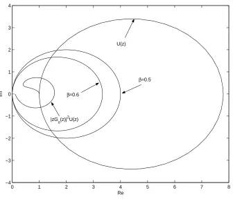
Note: Simple calculations indicate that the frequency domain conditions have a simple and easily checked graphical interpretation, namely that:
The plot of the frequency response function|G0(z)|2U(z) on the unit circle |z| = 1lies in the
interior of the circle of centreβ1 and radius β1
Recent work by the authors [4] using the inverse model algorithm produced the condition:
|1
β −U(z)|<
1
β ∀z∈ {z:|z|= 1} (52)
At its simplest level, the difference between the two results is the replacement ofU by|G0|2U. With
1. Both approaches require a strictly positive realU(z)for monotone robust convergence. This condition is connected very closely with the monotonicity property of the mean square error and it is expected, as with the inverse-model-based approach, that violation may lead to lack of convergence/instability. Another possibility is thatasymptoticconvergence may be retained but it may also be associated with error norm sequences that can increase from trial to trial.
2. In both cases, the positive real requirement onU(z)will tend to require that it is proper but not strictly proper i.e. thatGandG0have the same relative degree.
3. The gradient-based algorithm will however reduce performance limitations due to the effect of high frequency errors such as high frequency resonances in Gnot modelled in G0. In such
circumstancesU(z)will tend to take large gain values at frequencies close to these resonances. This will then require the use of small values of learning gainβto satisfy the monotone con-vergence criterion for the inverse model algorithm. This does not occur for the gradient-based algorithm because, in practice,Gis typically a low pass filter and hence bothG(z)andG0will
be small at high frequencies. The magnitude of|G0|2U will then be substantially reduced (as
compared withU) and permit increased learning gains leading to improved convergence rates.
4. In contrast with the beneficial high frequency effects of the gradient-based algorithm, it is possible that it could reduce performance if G (and hence G0) has a substantial resonance
peak within its bandwidth. A similar argument to the above suggests that the learning gains permitted will be reduced (as compared with the inverse model algorithm). As a consequence, it is desirable for a feedback control to be incorporated into the plant (and henceG) before the ILC analysis is undertaken. The feedback controller could be designed along classical lines and, in particular, designed to remove or reduce the resonance peak. In such circumstances, the high frequency benefits of the gradient-based approach indicate that it will, in practice, often be superior to the inverse-model algorithm in terms of its performance and robustness.
5. The above analysis has considered a specific uncertaintyU. It can easily be extended to cover sets of multiplicative uncertainties such as any subset of all proper multiplicative uncertainties satisfying an inequality of the form
|β1∗ − |G0(z)|2U(z)|<
1
β∗ ∀z∈ {z:|z|= 1} (53)
In conclusion, the analysis of monotone convergence has been seen to have elegant solutions in terms of inequalities between matrix representations of the plant and associated models. These inequalities can be converted into simple frequency domain (sufficient) conditions that indicate that the gradient-based approach has real potential for both performance and robustness.
Finally, note that, whenU(z) ≡ 1 and henceUe = I, the above results produce conditions for monotone convergence when there is no plant-model mismatch.
− − − − − − − − − − − − − − − − − − − − − − − − − − − − − − − − − − − − − − −
Corollary:Under the conditions of the theorem above, monotone convergence to zero is achieved in the absence of modelling errors if0< β||G||2∞<2where||G||∞= sup|z|=1|G(z)|is the familiar
H∞norm ofGon{z:|z| ≥1}.
− − − − − − − − − − − − − − − − − − − − − − − − − − − − − − − − − − − − − − −
Proof:SettingU =I,U(z)≡1andG0(z)≡G(z)in the previous result, monotone convergence
follows if|β1 − |G(z)|2|< β1 ∀z∈ {z:|z|= 1}. The result follows from simple complex algebra. 2
In particular, the result shows that, in the absence of mismatch, monotone convergence is not dependent on the phase characteristics of the plant (an observation that links these results to the continous-time methodology described in [12]).
8
Gradient-based Parameter Optimal ILC (POILC)
In [10], the benefits of using parameter optimization-based approaches to ILC design were introduced. A review of these ideas is provided in the IFAC Review article [11] with some extensions in the Automatica paper [6]. The basis of the parameter optimal ILC approach (POILC) is to examine the feedforward control update law
uk+1=uk+βk+1Kek (54)
whereK is a fixed matrix operation on the time seriesek andβk+1 is aniteration-dependentgain.
The resultant error dynamics is described by
ek+1 = (I−βk+1GK)ek (55) The learning gainβk+1is chosen to minimize an objective function of the quadratic form
where the proposed form of the weightwk+1is iteration dependent i.e.
wk+1 =w1+w2||ek||2, w1≥0, w2≥0, w1+w2>0 (57)
A simple calculation indicates that the required choice ofβk+1is just
βk+1=
eTkGKek
wk+1+||GKek||2
(58)
and optimality ensures that the mean square error is reduced monotonically from iteration to iteration i.e.
||ek+1||2 ≤ ||ek||2 ∀k≥0 (59) with equality holding if, and only if,βk+1 = 0.
In addition, using the results of [10] and [6], convergence of the error to zero is guaranteed for all initial input guessesu0 (and hence all initial errors e0) if, and only if, the symmetric part ofGK is
strictly positive or strictly negative definite. This is guaranteed for the gradient-based algorithm with zero modelling errorG=G0but may not be the case for the case of non-zero modelling error.
The case of non-zero modelling error setsK = GT0 but, as the plant modelGis presumed not known, the gain parameter cannot be updated using the above formula. It can however be estimated in a natural way ifβk+1 is obtained by replacingGby G0 i.e. the implemented gain is computed
from the formula
βk+1 =
eTkG0GT0ek
wk+1+||G0GT0ek||2
= ||G
T
0ek||2
w1+w2||ek||2+||G0GT0ek||2
(60)
The ideas used in the analysis of the fixed main parameter case can now be used to prove the following theorem :
− − − − − − − − − − − − − − − − − − − − − − − − − − − − − − − − − − − − − − −
Theorem (Robust Monotone Convergence of POILC):The gradient-based ILC parameter op-timal algorithm described above has the mean square error monotonicity property that, on iteration
k+ 1,||ek+1||<||ek||(independent ofek) if, and only if, the matrix representationUeof the multi-plicative modelling error satisfies the matrix inequality
Ue+UeT > βk+1G0TUeTUeG0>0 (61)
In addition, if
ˆ
β= sup{β = ||G T
0e||2
w1+w2||e||2+||G0GT0e||2
:||e|| ≤ ||e0||} (62)
and
then0< βk+1 ≤β,ˆ ∀k≥0and the error sequence{ek}k≥0 is guaranteed to converge
monotoni-cally in mean square norm to zero.
− − − − − − − − − − − − − − − − − − − − − − − − − − − − − − − − − − − − − − −
The matrix inequality can be converted into a frequency domain condition in a similar manner to the constant gain case to obtain:
− − − − − − − − − − − − − − − − − − − − − − − − − − − − − − − − − − − − − − −
Corollary (POILC - A Frequency Domain Condition):The mean square error sequence con-verges to zero monotonically if (a sufficient condition)
|1ˆ
β − |G0(z)|
2U(z)|< 1
ˆ
β ∀z∈ {z:|z|= 1} (64)
Equivalently, it is sufficient that the plot of the frequency response function|G0(z)|2U(z)on the unit
circle|z|= 1lies in the interior of the circle of centre1/βˆand radius1/βˆ.
− − − − − − − − − − − − − − − − − − − − − − − − − − − − − − − − − − − − − − −
Proof of above Theorem: Monotonicity on the(k+ 1)th iteration follows in a similar manner to the proof of monotonicity for the constant gain case. The replacement ofβk+1 byβˆalso ensures
monotonicity for all iterations as an induction argument indicates clearly that0 < βk+1 ≤ βˆfor all
k≥0. The theorem and corollary are hence proved if it can be proved that the error sequence always converges to zero. At optimality, it is easily seen that
||ek+1||2=||ek||2−βk+1eTkG0(Ue+UeT −βk+1UeTG0TG0Ue)GT0ek (65) and hence
||ek+1||2 ≤ ||ek||2−βk+1eTkG0(Ue+UeT −βUˆ eTGT0G0Ue)GT0ek (66) The assumptions of the theorem guarantee the existence ofǫ >0such that
||ek+1||2 ≤(1−βk+1ǫ)||ek||2, ∀k≥0 (67) If{ek}k≥0 does not converge to zero, then it is easily seen that lim supk→∞βk+1 ≥ δ for some
δ >0. It follows that||ek||2 ≤(1−δǫ)k||e0||2and hence thatekconverges to zero. The theorem is now proved as this is a contradiction.2
parameter optimal ILC algorithm. They are hence not repeated here for brevity. Two new observations are however worthy of emphasis:
1. Noting that, withw1andw2fixed,lim||e0||→0βˆ= 0. It follows that robustness of the parameter optimal algorithm increases as the initial errore0 decreases i.e. a good initial input guessu0
will improve the robustness of the methodology considerably.
2. Also, withe0 6= 0fixed,lim|w1|+|w2|→∞βˆ= 0and hence an increase in either of the weights will tend to increase the robustness of the algorithm. Increasing weights is expected however to reduce performance by slowing convergence rates.
The estimation of an appropriate value forβˆcan be approached as summarised in the next section.
9
Estimation of
β
ˆ
To estimateβˆ, note that the supremum in
ˆ
β= sup{β(e) = ||G T
0e||2
w1+w2||e||2+||G0GT0e||2
:||e|| ≤ ||e0||} (68)
is achieved on the boundary eTe = ||e
0||2. It is therefore described by stationary points of the
Lagrangian
L=β(e) +λ(eTe−eT0e0) =
eTM e
w1+w2eTe+eTM2e
+λ(eTe−eT0e0) (69)
where, for simplicityM =G0GT0. the stationary points are described by the equations ∂L∂λ = 0and ∂L
∂e = 0i.e.eTe=eT0e0 and
2
·
M e
w1+w2eTe+eTM2e−
eTM e
(w1+w2eTe+eTM2e)2
(w2e+M2e) +λe
¸
= 0 (70)
which is just
£
βM−β2(w2I+M2) +λeTM e
¤
e= 0 (71)
A spectral argument then indicates that, if M has eigenvalues 0 < σ2(G0) = σ12 ≤ σ22· · · ≤
σ2N+1−k∗ =σ2(G0)(the squared singular values ofG0), then, for someσj,
βσ2j −β2(w2+σj4) +λeTM e= 0 (72) In addition,
Using the definition ofβ to eliminateeTM2eimplies that
β2w1+λeTM e||e0||2 = 0 (74)
and, eliminatingλgives the desired formula forβˆ
ˆ
β = σ
2
j||e0||2
w1+w2||e0||2+σ4j||e0||2
(75)
The remaining question is to estimate the relevantσjto maximizeβˆ. This could be done by numerical search mechanisms but a simpler approach uses an examination of the continuous function
f(µ) = µ||e0||
2
w1+w2||e0||2+µ2||e0||2
(76)
in the rangeµ∈[0,+∞). This function is positive with a single stationary point (a maximum) when
||e0||2µ2 =w1+w2||e0||2withf(µ) = 2(w ||e0||
1+w2||e0||2)1/2. Introducing the necessary constraint that
µ∈[σ2(G0), σ2(G0)]it follows that the value ofβˆis defined by three relations:
Case 1:If||e0||2σ4(G0)≥w1+w2||e0||2then
ˆ
β= σ
2(G
0)||e0||2
w1+w2||e0||2+σ4(G0)||e0||2
(77)
Case 2:If||e0||2σ4(G0)≤w1+w2||e0||2then
ˆ
β= σ
2(G
0)||e0||2
w1+w2||e0||2+σ4(G0)||e0||2
(78)
Note: This is trivially satisfied ifw2 > σ4(G0). A sufficient condition for this is thatw2 >||G0||4∞
which can be computed from the transfer functionG0.
Case 3:In all other cases
ˆ
β ≤ ||e0||
2(w1+w2||e0||2)1/2
(79)
the right-hand-side of the inequality being a very good estimate of the actual value ifN is large and the valuesσj2+1−σj2are all small (relative toσ2(G0)).
Note the following observations:
1. As the above estimate is a monotonically increasing function of ||e0||, it indicates that the
parametersw1andw2play different roles in robustness. This is because it is always possible to
regardekas the initial iteration for the rest of the algorithm. In principle a value ofβˆ(denoted ˆ
asymptotically. Case2is however always valid asymptotically and is valid for all iterations if
w2 > σ4(G0). Otherwise case3may play a role in earlier iterations.
If w1 = 0, the estimated βˆremains constant at the value 1 2w21/2
i.e there is no change in the robustness conditions. If w2 = 0then clearlyβˆkcomputed at this iteration will converge to zero as k → ∞ i.e. the region of permissible uncertainty increases. This can be explained intuitively by thinking of the introduction of the term in w2 as a systematic reduction of w1
from iteration to iteration. Such a reduction tends to increase the value of the learning gain and hence potentially increase performance. The price paid for this bonus is that the range of permitted modelling error does not increase with iteration index.
2. For a givenU(z)satisfying the POILC robustness conditions for a known value ofβˆ, the for-mula can alternatively be used to provide candidate weightsw1andw2to satisfy the inequality
ˆ
β ≥ ||e0||
2(w1+w2||e0||2)1/2. the discussion above of the relative effects ofw1andw2will, in princi-ple, aid this choice.
10
Use of Exponential Norms
In the paper [4], the results for the mean square error were extended to ("exponentially") weighted norms of the form
||f||ǫ=||Ef||=
q
ΣN+1−k∗
j=1 ǫ2(j−1)fj2 =||fǫ|| (80) induced by the inner producthf, giǫ =fTETEg=fǫTgǫ. Hereǫ >0,E=diag(1, ǫ, ǫ2, . . . , ǫN−k∗) andfǫ =Ef(with elementsfǫ,j =fjǫj−1) is the exponentially weighted time series vector obtained from the time series vectorf. Any algorithm that guarantees monotonic convergence of the weighted norm to zero also ensures that the mean square error will also converge to zero (as all norms on
For simplicity. letk∗≥1and define modified model matrices as follows
Gǫ =EGE−1 =
CAk∗−1
B 0 0 . . . 0
ǫCAk∗
B CAk∗−1
B 0 . . . 0
ǫ2CAk∗+1
B ǫCAk∗B CAk∗−1
B . . . 0 ..
. ... ... . .. ...
ǫN−k∗
CAN−1B ǫN−k∗−1
CAN−2B . . . CAk∗−1
B (81)
(with similar definitions forG0,ǫ = EG0E−1 andUe,ǫ =EU E−1). A simple calculation indicates that the process model then takes the formyǫ =Gǫuǫ+dǫwith the reference signalrreplaced byrǫ andekreplaced byeǫ,k =rǫ−yǫ,k.
The natural input update law for a constant gain gradient-based algorithm for an exponentially weighted norm takes the form
uǫ,k+1=uǫ,k+βGT0,ǫeǫ,k (82) The results of the previous sections can be applied to this formulation to obtain necessary and suf-ficient conditions for robust monotone convergence with respect to the ǫ-norm in terms of matrix inequalities associated with the appropriate matrix representations ofG0,ǫandUe,ǫ. More usefully, as the exponentially weighted signals are associated with transfer functionsGǫ(z) =G(zǫ−1)ǫ−k
∗ ,
G0ǫ(z) =G0(zǫ−1)ǫ−k
∗
andUǫ(z) =U(zǫ−1)the frequency domain condition for robust monotone convergence with respect to the weighted norm|| · ||ǫbecomes
|β1 − |G0ǫ(z)|2Uǫ(z)|< 1
β, ∀|z|= 1 (83)
or, equivalently,
|β1 −ǫ−2k∗|G0(z)|2U(z)|<
1
β, ∀|z|=ǫ
−1 (84)
i.e. the unit circle is replaced by a circle of radiusǫ−1 and the extra factor ofǫ−2k∗
appears in the inequality. The Principle of the Maximum indicates that reducingǫwill increase the range of values ofβ that satisfy this condition. In practical terms, this implies that increased values of the learning gain are permitted if increases in the mean square error can be tolerated before convergence to zero is achieved. Lettingǫ→ 0+, it is easily seen thatUǫ(z) approaches the valueU(∞)uniformly on the region{z : |z| ≥ 1} and henceUǫ(z) is positive real for all sufficiently small values ofǫ if
U(∞)>0. It follows that if the condition
|β1 − |G∗0(∞)|2U(∞)|< 1
is satisfied then the algorithm is robust monotone convergent with respect to allǫ-norms in a some non-empty range0 < ǫ < ǫ∗. Interpreting|G∗
0(∞)|2U(∞) = G0(∞)G(∞)as the product of high
frequency gains, it is typically seen to be very small. The possibility of using higher learning gainsβ
follows immediately.
It is expected that the implemented form of the algorithm will use unweighted rather than expo-nentially weighted signals. The real input update formula is easily seen to be
uk+1 =E−1uǫ,k =uk+βE−1GT0ǫEek=uk+βGT0ǫ2ek (86) and hence is computed using the time reversed response of a linear systemG0ǫ2 to the time reversal ofek. For simulation purposes this linear system is obtained fromG0using the map(A, B, C, D)7→
(ǫ2A, ǫ2B, ǫ−2k∗
C, ǫ−2k∗
D).
The above analysis can be extended to the case of POILC using the modified problem
uǫ,k+1=argmin{||eǫ,k+1||2+wk+1β2k+1} (87)
subject to the constraints
uǫ,k+1 =uǫ,k+βk+1GT0ǫeǫ,k, yǫ,k+1 =G0ǫuǫ,k+1+dǫ (88) The solution to this problem is seen to be
uk+1=uk+βk+1GT0ǫ2ek, βk+1 =
||GT
0ǫeǫ,k||2
wk+1+||G0ǫGT0ǫeǫ,k||2
(89)
where, after some manipulation, the identitiesGT0ǫeǫ,k = EGT0ǫ2ek andG0ǫGT0ǫeǫ,k = EG0GT
0ǫ2ek give the formula
βk+1 = ||
GT
0ǫ2ek||2ǫ
wk+1+||G0GT0ǫ2ek||2ǫ
(90)
The control update law and parameter choice are now related in terms of the two modelsG0andG0ǫ2. These models are used, with appropriate simulations, to undertake all computations.
11
Illustrative Example
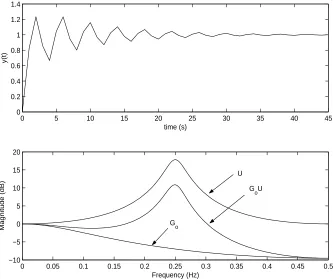
To illustrate the results of the above theory, a simple example is constructed using a plant modelG(z) constructed to contain simple nominal first order dynamics with a high frequency resonance defined by the parameterized data
G0(z) = 1−γ
z−γ, U(z) =
(z2+a) (z2+λ2)
(1 +λ2)
Although a theoretical example, the authors believe that it represents similar performance problems to those that are be met in applications to mechanical systems where available nominal models do not include structural high frequency resonances. For simplicity, the data is normalized so thatG0(1) =
G(1) = U(1) = 1and0 < λ < 1. Clearly, the relative degree ofG0(z)isk∗ = 1and it is easily
checked thatU(z)is positive real (i.e. its Nyquist plot lies in the open right-half complex plane) for
a∈(−1,1).
For illustrative purposes, chooseλ= 0.9,a= 0.1andγ = 0.5. For reasons of space, the50×50 matrix representations ofG(z),G0(z) andU(z) are not presented here. The unit step response of
Gis provided in Fig. 1, top graph, with the Bode plots ofG, G0 andU plotted in Fig. 1, bottom
graph. The high frequency resonance inGis clearly seen. As this phenomenon is not modelled in
G0,U has a substantial resonance at a frequency well beyond the bandwidth of the nominal model
(substantiated by the simple hand calculationU(i) = 9.5).
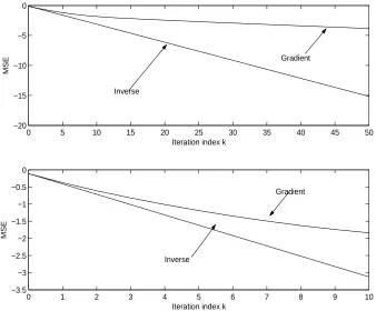
Two fixed gain algorithms are considered, namely the inverse-model algorithm and the gradient-based algorithm
uk+1 =uk+βG0−1ek, β = 0.5 (92)
uk+1 =uk+βG0Tek, β= 0.6 (93) with initial control input supervectoru0= 0. These algorithms are first applied to the nominal model
G0with the parametersβ(shown above) being chosen in each case to achieve an approximate halving
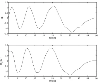
of the tracking error from iteration to iteration. Zero initial conditions are assumed and the demanding reference signal,0≤j≤50,
r(j) =
·
1 + 0.1 sin(20πj 50 )
¸
cosh(j/50) sin(6π
·
j
50(2−
j
50)
¸
) (94)
is chosen as a growing exponential oscillation with variable, increasing frequency and additional amplitude modulation (see Fig. 2). The signal is believed to be demanding as it contains a sufficiently rich frequency content to ensure that the high frequency resonance will ultimately be excited.
The simulation results are shown in Fig. 3 for the first 50 iterations (top graph) and for he first 10 iterations (bottom graph). This figure plots the superimposed logarithmic mean square error log10£
(N +k∗−1)−1eTkek
¤
0 5 10 15 20 25 30 35 40 45 0
0.2 0.4 0.6 0.8 1 1.2 1.4
time (s)
y(t)
0 0.05 0.1 0.15 0.2 0.25 0.3 0.35 0.4 0.45 0.5
−10 −5 0 5 10 15 20
Frequency (Hz)
Magnitude (dB)
U
G oU
[image:25.595.139.472.74.353.2]G o
Figure 1: Step response and Bode plots
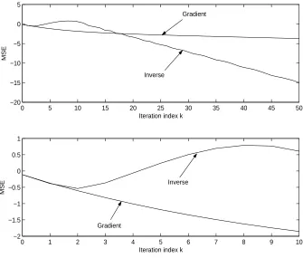
1. The inverse-model-based algorithm suffers from substantial increases (around10-fold in mag-nitude) in the mean square error in iterations5−10. This is regarded as a substantial overall degradation in performance as, for most practical situations the large errors involved will be unacceptable and possible even disastrous for systems operation. The situation does begin to improve after around15iterations with ultimate rapid convergence to zero. In practice, the op-erator would have terminated the method before this iteration and hence, despite the ultimately rapid asymptotic convergence, it is concluded that the modelling error has induced unaccept-able behaviour. The inverse-model-based algorithm should be regarded as having failed.
2. The gradient based algorithm copes much better with the modelling error present, producing monotonic mean square errors and only a minor degradation in performance (as seen in Fig. 4). Fig. 5 shows the FFT of the initial error (the reference signal) and that of the final error at iteration 50 whilst Fig. 6 shows the the time series for the final error. It is seen that the algorithm has successfully learnt to track the reference to a high accuracy over the bandwidth of the plant although learning of the high frequency component is slow.
0 5 10 15 20 25 30 35 40 45 50 −1.5
−1 −0.5 0 0.5 1 1.5
time (s)
r(t)
0 5 10 15 20 25 30 35 40 45 50
−1.5 −1 −0.5 0 0.5 1 1.5
time (s)
(G
o
U)
−1
[image:26.595.139.474.70.360.2]r
Figure 2: Reference signalr(t)and optimal inputu∗ = (GoU)−1r
be explained by plotting the "Nyquist" plots of the two frequency response functions U(z) and
|G0(z)|2U(z) in the complex plane with their associated circles of centre β and radius β
super-imposed. these are shown in Fig. 7. Note that the plot ofU(z)leaves its circle hence violating the inverse model condition for robust monotone convergence [4]. In contrast, the plot of|zG0(z)|2U(z)
is contained within the circle and hence robust monotone convergence is guaranteed by the results of this paper (and has been seen in the simulation results).
Note that the gradient-based algorithm has also been applied successfully to industrial systems. Details of this work can be found from [5] and [2] where similar conclusions are reached on the bases of observed experimental data.
12
A Note on Series Compensation
0 5 10 15 20 25 30 35 40 45 50 −20
−15 −10 −5 0
Iteration index k
MSE
0 1 2 3 4 5 6 7 8 9 10
−3.5 −3 −2.5 −2 −1.5 −1 −0.5 0
Iteration index k
MSE
Inverse
Gradient
Gradient
[image:27.595.137.475.73.353.2]Inverse
Figure 3: Convergence behaviour in the nominal case
domain conditions for robust monotone convergence become
|β1 − |G0(z)K(z)|2U(z)|< 1
β ∀z∈ {z:|z|= 1} (95)
which clearly indicates the potential to usefully useK(z)to shape the gain characteristics of either
G0(z)K(z)or|K(z)|2U(z)and hence|G0(z)K(z)|2U(z). For example, the use of notch filters may
permit robustness to be increased by reducing the effects of residual resonances inG0. Alternatively,
they could be used to cancel the effects of resonances in the mismatchU(z). Note that the phase characteristics ofK(z)do not affect the robust monotone convergence analysis.
Finally an alternative matrix description of the modified algorithm is as follows: consider the typical case whenK(z)has relative degree zero and suppose thatKis its matrix representation, then the update law takes the form
0 5 10 15 20 25 30 35 40 45 50 −20
−15 −10 −5 0 5
Iteration index k
MSE
0 1 2 3 4 5 6 7 8 9 10
−2 −1.5 −1 −0.5 0 0.5 1
Iteration index k
MSE
Inverse
Gradient
Inverse
[image:28.595.138.473.73.358.2]Gradient
Figure 4: Convergence behaviour with uncertainty
0 0.05 0.1 0.15 0.2 0.25 0.3 0.35 0.4 0.45 0.5
−160 −140 −120 −100 −80 −60 −40 −20 0 20
Frequency (Hz)
[image:28.595.137.471.408.696.2]Power spectrum (dB)
0 5 10 15 20 25 30 35 40 45 50 −8
−6 −4 −2 0 2 4 6 8x 10
−4
time (s) e50
[image:29.595.137.474.74.374.2](t)
Figure 6: Time series ofe50(t)
13
Conclusions
The paper has provided a complete analysis of the robust monotone convergence of a gradient-based Iterative Learning Control algorithm in terms of necessary and sufficient matrix inequalities and fre-quency domain conditions that can be easily checked in terms of plant model and modelling error transfer functions. The method of analysis was the use of matrix models relating the time series of input, output and error signals. A complete analysis of these models is provided which demonstrates that the relative degree of the plant and model are crucial parameters in the analysis of ILC dynamics and hence, it is argued, in the construction of feedforward learning laws. In addition, they clearly show that the use of the "non-causal" gradient operator can be implemented using a plant model and time reversal operations i.e. state space models rather than the matrix models used in the analysis are all that is required for implementation purposes.
0 1 2 3 4 5 6 7 8 −4
−3 −2 −1 0 1 2 3 4
Re
Im
U(z)
β=0.5
β=0.6
|zG o(z)|
[image:30.595.140.476.70.365.2]2 U(z)
Figure 7: Nyquist plots
The benefits of the approach have also been shown to transfer to the use of Parameter-Optimal ILC with the additional benefits that robustness can be improved by either ensuring that the initial tracking error is small and/or by using larger weighting coefficients in the quadratic objective function chosen. The analysis provides formulae that can guide the application of these principles although more experience in the choice of weights will be needed to aid inexperienced practitioners.
In a similar manner to [4], the use of exponentially weighted norms has been analysed with a view to using monotonicity of these norms as a design principle. Stability and the ideas of robust monotone convergence extend trivially to this case which, with0 < ǫ < 1, can be regarded as a relaxation of the ideas of robust monotone convergence (with respect to the mean square error) to permit some increases in mean square error in initial iterations whilst still ensuring asymptotically convergent learning.
References
[1] S. Arimoto, S. Kawamura, and F. Miyazaki. Bettering operations of robots by learning.Journal of Robotic Systems, 1:123–140, 1984.
[2] S. Daley, J. Hätönen, and D.H. Owens. Hydraulic servo system command shaping using iterative learning control. InProceedings of the UKACC Conference, Control 2004, Bath, UK, 2004.
[3] K. Furuta and M. Yamakita. The design of learning control systems for multivariable systems. InProceedings of the IEEE International Symposium on Intelligent Control, pages 371–376, Philadelphia, Pennsylvania, U.S.A., 1987.
[4] T.J. Harte, J. Hätönen, and D.H. Owens. Discrete-time inverse model-based iterative learning control: stability, monotonicity and robustness. International Journal of Control, 78(8):577– 586, 2005.
[5] J. Hätönen, T.J. Harte, D.H. Owens, J. Ratcliffe, P. Lewin, and E. Rogers. A new robust iterative learning control law for application on a gantry robot. InProceedings of the 9th IEEE conference on Emerging Technologies and Factory Automation, Lisbon, Portugal, 2003.
[6] J. Hätönen, D.H. Owens, and K. Feng. Basis functions and parameter optimisation in high-order iterative learning control. Automatica, 2005. In press.
[7] J. Hätönen, D.H. Owens, and K.L. Moore. An algebraic approach to iterative learning control. International Journal of Control, 77(1):45–54, 2004.
[8] K. Kinosita, T. Sogo, and N. Adachi. Iterative learning control using adjoint systems and stable inversion. Asian Journal of Control, 4(1):60–67, 2002.
[9] K.L. Moore. Iterative Learning Control for Deterministic Systems. Springer-Verlag, 1993.
[10] D.H. Owens and K. Feng. Parameter optimization in Iterative Learning Control. International Journal of Control, 76(11):1059–1069, 2003.
[11] D.H. Owens and J. Hätönen. Iterative learning control - an optimization paradigm. Annual Reviews in Control, 29(1):57–70, 2005.