This is a repository copy of
Identification of Nonlinear Parameter-Dependent
Common-Structured models to accommodate varying experimental conditions and design
parameter properties
.
White Rose Research Online URL for this paper:
http://eprints.whiterose.ac.uk/74595/
Monograph:
Wei, H.L., Lang, Z.Q. and Billings, S.A. (2006) Identification of Nonlinear
Parameter-Dependent Common-Structured models to accommodate varying experimental
conditions and design parameter properties. Research Report. ACSE Research Report no.
935 . Automatic Control and Systems Engineering, University of Sheffield
[email protected] https://eprints.whiterose.ac.uk/
Reuse
Unless indicated otherwise, fulltext items are protected by copyright with all rights reserved. The copyright exception in section 29 of the Copyright, Designs and Patents Act 1988 allows the making of a single copy solely for the purpose of non-commercial research or private study within the limits of fair dealing. The publisher or other rights-holder may allow further reproduction and re-use of this version - refer to the White Rose Research Online record for this item. Where records identify the publisher as the copyright holder, users can verify any specific terms of use on the publisher’s website.
Takedown
If you consider content in White Rose Research Online to be in breach of UK law, please notify us by
Identification of Nonlinear Parameter-Dependent
Common-Structured Models to Accommodate Varying Experimental
Conditions and Design Parameter Properties
Hua-Liang Wei, Zi-Qiang Lang and Stephen A. Billings
Research Report No. 935
Department of Automatic Control and Systems Engineering
The University of Sheffield
Mappin Street, Sheffield,
S1 3JD, UK
Identification of Nonlinear Parameter-Dependent
Common-Structured Models to Accommodate Varying Experimental
Conditions and Design Parameter Properties
Hua-Liang Wei, Zi-Qiang Lang and Stephen A. Billings
Department of Automatic Control and Systems Engineering, University of Sheffield Mappin Street, Sheffield, S1 3JD, UK
8 August 2006
Abstract: This study considers the identification problem for a class of nonlinear parameter-varying
systems associated with the following scenario: the system behaviour depends on some specifically prescribed parameter properties, which are adjustable. To understand the effect of the varying parameters, several different experiments, corresponding to different parameter properties, are carried out and different data sets are collected. The objective is to find, from the available data sets, a common parameter-dependent model structure that best fits the adjustable parameter properties for the underlying system. An efficient common model structure selection (CMSS) algorithm, called the extended forward orthogonal regression (EFOR) algorithm, is proposed to select such a common model structure. Several examples are presented to illustrate the application and the effectiveness of the new identification approach.
Keywords: Forward orthogonal regression, nonlinear system identification, parameter-dependent
model.
1. Introduction
a special case of internal-parameter-dependent (IPD) models, where the dynamical behaviour of the model is directly affected by changes of the internal parameters.
In terms of system identification, the task for general IPD model identification problems can be summarized as follows. By setting the process internal parameters to be different values, a number of experiments are carried out on the same system, and different data sets are obtained, corresponding to different parameter properties. The objective is to find from the available data a parsimonious common model structure, to accommodate all the different parameter properties by best fitting all the data sets using the common structured model, with varying process internal parameters. This is different from conventional parameter-varying models, where process internal parameters are assumed to be time-varying.
There are many other cases where parameter-dependent models are desirable. Consider the following scenario. In typical normal operating conditions, the dynamical behaviour of an underlying system is often determined by the system model structure and the associated process internal parameters. In many cases, however, several external parameters, for example temperature, pressure intensity, light illumination, geometry shape and size, etc., may also indirectly affect the dynamical behaviour of the system, via the associated process internal parameters. In order to fully understand the mechanisms of the underlying dynamics under different operating conditions, several experiments, with respect to different exogenous parameter properties, may be required. The task of external-parameter-dependent (EPD) model identification is to find a best common model structure based on the available data, to accommodate the effects of all the external parameters, by best fitting all the data sets using the common structured model, with adjustable process internal parameters. This is related to but distinct from the concepts of spatial piecewise linear models and models with single dependent parameters (Billings and Voon 1987).
For convenience of description, in the following all non-internal parameters, including different experimental conditions, will be referred to as external or exogenous parameters. Specifically prescribed parameters, either internal or exogenous, will be called experiment parameters or design parameters. This work involves several abbreviations and these are collected in the appendix to facilitate reading of text.
2. The concept of the parameter-dependent commonly structured model
The parameter-dependent common-structured (PDCS) model is defined as below )) ( ), ( , ), 1 ( ), ( , ), 1 ( ( )
(t f y t y t ny u t u t nu
y = − − − − +e(t) (1) where
•
the nonlinear mapping f is often unknown and needs to be identified from given observations of the input u(t)and the outputy(t);n
uand ny are the maximum input and output lags; e(t) is the model prediction error, which can often be treated as an independent zero mean noise sequence providing that the function f gives a sufficient description of the system.•
( )∈Θ represents an internal parameter vector, which is a function of the external parameter set ∈Ω, where Θand Ω are the internal and external parameter sets, respectively. The external parameter set may not explicitly appear in the model but does indirectly affect the dynamical behaviour of the model through the internal parameter .Assume that a total of K experiments, corresponding to K different cases of exogenous parameter properties, 1, 2,, K, have been completed on the same system, model (1) can then be expressed in a more explicit form as
t. s. , ) ), ( , ), 1 ( ), ( , ), 1 ( ( t. s. ), ), ( , ), 1 ( ), ( , ), 1 ( ( t. s. ), ), ( , ), 1 ( ), ( , ), 1 ( ( )
( 2 2
2 1 1 1 − − − − − − − − − − − − = K K u y K u y u y n t u t u n t y t y f n t u t u n t y t y f n t u t u n t y t y f t y (2)
where fi(⋅)(i=1,..,K) are different linear or nonlinear functions that share a common structure in representation. The symbol ‘s.t. i’ means the individual model is subject to the exogenous parameter
i . Clearly, if K=1, the PDCS model (2) will reduce to the traditional NARX (Nonlinear
AutoRegressive with eXogenous inputs) model (Leontaritis and Billings 1985, Pearson 1999).
structure, where each subsystem model may not need to share the same common model structure, and which often involves one single data set.
3. The identification of the commonly structured model
3.1 The linear-in-the-parameters regression model
The nonlinear mapping f in (1) can be constructed using a variety of local or global basis functions including polynomials, kernel functions, splines, radial basis functions, neural networks and wavelets (Chen and Billings 1990, Kavli 1993, Berger 1994, Wu and Harris 1997, Pearson 1999, Liu 2001, Harris et al. 2002, Chen et al. 2005, Billings and Wei 2005). One of the most popular representations is the polynomial model (Leontaritis and Billings 1985), which takes the form below
∑
∑ ∑
= = = + + + = d i d i i i i i i d i ii x t f x t x t
f t y 1 1 0
1 2 1
2 1 2 1 1 1
1( ( )) ( ( ), ( )) ) ( θ ) ( )) ( , ), ( ), ( ( 1 2 1 2 1 1 1 t e t x t x t x f i d i i i i i i i d i + +
∑
∑
− = = (3)
where
m
i i i12
θ
are parameters, d =ny+nu and
∏
= = m k i i i i i i i i ii x t x t x t x t
f k m m m 1 ) ( )) ( , ), ( ), ( ( 2 1 2 1 2
1 θ , 1≤m≤ (4)
≤ ≤ + − − ≤ ≤ − = d k n n k t u n k k t y t x y y y k 1 )) ( ( 1 ) ( )
( (5)
The degree of a multivariate polynomial is defined as the highest order among the terms, for example, the degree of the polynomial h(x1,x2,x3)=a1x14 +a2x2x3 +a3x12x2x32 is determined by the term
2 3 2 2 1x x
x and thus=2+1+2=5. Similarly, a NARX model with a nonlinear degree means that the order of each term in the model is not higher than.
A NARX model constructed using basis function expansions can often be expressed using a linear-in-the-parameters form ) ( ) ( ) ( 1 t e t t y M m m m + =
∑
= φθ
(6)
where M is the total number of candidate regressors, φm(t) =φm( tx( ))(m=1,2, …, M) are the model
3.2 The multiple regression model
Assume that a total of K experiments, corresponding to K different cases of the experiment parameter properties, have been carried out on the same system, and K different data sets, with respect to the K experiments, have been obtained. Also, assume that a common model structure, with the form of (6), can best fit all the data sets. Denote the input and the output sequence for the kth experiment by Nk
t k t
u ( )} 1
{ = and Nk
t k t
y ( )} 1
{ = , respectively, for k=1,2,…, K. The kth predictor vector is thus given by
T d k k
k(t)=[x ,1(t),x , (t)]
x =[yk(t−1),,yk(t−ny), T u k
k t u t n
u ( −1),, ( − )] . It is assumed that all the
K data sets can be represented using a common model structure, with a different parameter set,
deduced from the initial candidate regression model below
) ( )) ( ( )
(
1
, t e t
t
y k
M
m
k m m k
k =
∑
+=
x φ
β ( ) ( )
1 ,
, t ek t M
m
m k m
k +
=
∑
= φ
β
(7)
This can be expressed using a compact matrix form
k k k
k e
y =Φ + (8) whereyk =[yk(1),,yk(Nk)]T,
T M k k
k =[β ,1,,β , ] ,
T k k k
k =[e (1),,e (N )]
e ,and Φk =[ k,1,, k,M] with k,m=[φk,m(1),,φk,m(N )]k T for k=1,2, …, K and m=1,2,…, M.
For large lags n andy n , the regression model (7) often involves a large number of candidate u
model terms, even if the nonlinear degree is not very high, say=2 or =3. Experience has shown that an initial candidate model with a large number of candidate model terms can often be drastically reduced by including in the final model only the effectively selected significant model terms. Furthermore, a simple concise model is usually desirable for practical applications including system analysis, design, control and prediction. This is one of the motivations of the present study to select significant model terms to form a parsimonious common model structure.
3.3 The extended forward orthogonal regression algorithm
A new common model structure selection (CMSS) algorithm, called the extended forward orthogonal regression (EFOR) algorithm, which is generalized from the standard orthogonal least squares (OLS) algorithm (Billings et al. 1989, Chen et al. 1989) and the recently developed forward orthogonal regression (FOR) algorithm (Wei and Billings 2006, Wei et al. 2006), will be designed for the PDCS identification problem.
that k,m=[φm(xk(1)),,φm(xk(N ))]i T (k=1,2, …,K). The common model structure selection problem
is equivalent to finding, from I, a subset of indices,In={im:m=1,2,,n,im∈I} wheren≤M, so that
i
y (i=1,2, …, K) can be approximated using a linear combination of
n
i i
i1, 2,, as i i i n i i i i
i n e
y =θ,1 ,1++θ, , + (9)
Following Billings et al. (1989) and Chen et al. (1989), a squared correlation coefficient will be used to measure the dependency between two associated random vectors. The squared correlation coefficient between two vectors x and y of size N is defined as
∑
∑
∑
= = = = = N i i N i i N i i i T T T y x y x C 1 2 1 2 1 22 ( )
) )( ( ) ( ) , ( y y x x y x y
x (10)
The squared correlation coefficient is closely related to the error reduction ratio (ERR) criterion defined in the standard orthogonal least squares (OLS) algorithm for model structure selection. A comprehensive discussion on OLS-ERR algorithm can be found in Billings et al. (1989) and Chen et al. (1989).
Letrk,0 =yk(k=1,2, …, K). For k=1,2, …, K and j=1,2, …, M, calculate c1(k,j)=C(yk, k,j),
and define =
∑
= ≤ ≤ K k Mj K c k j
s
1 1 1
1 ( , )
1 max
arg (11)
The first significant common model term can then be selected as the s1th element, φs1, in the
dictionary D. Accordingly, the first significant basis vector for the kth regression model is thus 1
, 1 , ks
k = , and the first associated orthogonal basis vector can be chosen as qk,1= k,s1.The model
residual for the kth regression model, related to the first step search, is given as
1 , 1 , 1 , 1 , 0 , 0 , 1 , k k T k k T k k k q q q q r r
r = − (12)
Notice that c1(k,s1) can be viewed as the error reduction ratio (ERR) that is introduced by including the first basis vector
1
, 1 , ks
k = into the kth regression model. The criterion (11), by
maximizing the sum of the ERR values relative to all the K data sets, guarantees that the variation of the outputs in all the K data sets can be explained by including the model term
1
s
In general, the mth significant model term
m
s
φ can be chosen as follows. Assume that at the (m-1)th step, (m-1) significant model terms, φ1,φ2,φm−1, have been selected. Let k,1, k,2,, k,m−1be the
associated basis vectors for the kth regression model, and assume that the (m-1) selected bases have been transformed into a new group of orthogonal bases qk,1,qk,2,,qk,m−1via some orthogonal
transformation. Let
∑
− = − = 1 1 , , , , , , ) ( , m s s k s k T s k s k T j k j k m j k q q q qp , j∈Jm (13)
where Jm={j:1≤ j≤M,j≠st,1≤t≤m−1} . For k=1,2,…,K and j∈Jm , calculate cm(k,j)=
) , ( (,) m j k k
C y p , and define
=
∑
= ∈ K k m J jm c k j
K s m 1 ) , ( 1 max
arg (14)
The mth significant common model term can then be selected as the s th element, m φsm , in the
dictionary D. Accordingly, the mth significant basis vector for the kth regression model is thus
m
s k m
k, = , , and the first associated orthogonal basis vector can be chosen as
) ( , , m s k m
k p m
q = .The model residual for the kth regression model, related to the mth step search, is given as
m k m k T m k m k T m k m k m k , , , , 1 , 1 , , q q q q r r
r = − − − (15)
Subsequent significant bases can be selected in the same way step by step. Notice that the (m-1) basis vectors, k,1, k,2,, k,m−1 (respectively the associated orthogonalized bases, qk,1,qk,2,,qk,m−1), by
including the mth basis
m
s k m
k, = , (respectively the orthogonalized basis
) ( , , m s k m
k p m
q = ) , can explain the variation in the outputs of the K data sets with a higher percentage than by including any other candidate bases. The quantityAERR(m)=(1/K)
∑
kK=1cm(k,sm) is referred to as the mth average error reduction ratio (AERR).From (15), the vectors rk ,mand qk ,m are orthogonal, thus
m k T m k m k T m k m k m k , , 2 , 1 , 2 1 , 2 , ) ( || || || || q q q r r
r = − − − (16)
By respectively summing (15) and (16) for m from 1 to n, yields
n k n m m k m k T m k m k T m k k , 1 , , , , 1 , r q q q q r y
∑
= − +n k T n k n k T n k n k n k , , 2 , 1 , 2 1 , 2 , ) ( || || || || q q q r r
r = − − −
∑
= −
−
= n
m km
T m k m k T m k k
1 , , 2 , 1 ,
2 ( )
|| || q q q r
y (18)
From (17) and (18), the model residual rk ,n can be used to form a criterion for model selection, and
the search procedure will be terminated when the norm ||rk,n||2satisfies some specified conditions. In
the present study, an approximate minimum description length (AMDL) criterion developed by Saito (1994) and Antoniadis et al. (1997), on the basis of the Rissanen’s MDL criterion (Rissanen 1984), will be used to determine the model size. For the case of single regression model, AMDL is defined as
N N n n n 2 2 log 5 . 1 )] [MSE( log 5 . 0 )
AMDL( = +
N N n N n 2 2 2 log 5 . 1 || || log 5 .
0 +
= r (19)
where MSE is the mean-square-error from the associated model, N is the length of the associated training data set, n is the number of model terms, and r is the associated model residual. n
The present study uses the following average AMDL as the criterion to determine the number of common model terms
∑
= = K k k n K n 1 ] [ ) ( AMDL 1 )AAMDL( (20)
whereAMDL[k](n)is value for the AMDL criterion associated to the kth data set.
3.4 Parameter estimation
It is easy to verify that the relationship between the selected original bases k,1, k,2,, k,n and
the associated orthogonal basesqk,1,qk,2,,qk,n, for the kth data set, is given by
n k n k n
k, Q , R ,
A = (21) whereAk,n =[ k,1,, k,n], Qk ,n is an Nk×nmatrix with orthogonal columnsqk,1,qk,2,,qk,n, and
n k ,
R is an n×nunit upper triangular matrix whose entries uij(1≤i≤ j≤n) are calculated during the orthogonalization procedure. The unknown parameter vector, denoted by k,n =[θk,1,,θk,n]T, for the
model with respect to the original bases (similar to (9)), can be calculated from the triangular equation
n k n k n
k, , g ,
R = withgk,n=[gk,1,,gk,n]T , wheregm=(rkT,m−1qk,m)/(qTk,mqk,m) for m=1,2, …, n.
3.5 A general procedure for PDCS model identification
•
Collect K different data sets from K experiments.•
Select common model terms using the new EFOR-CMSS algorithm.•
Estimate relevant model parameters for each individual case of experiment parameters.•
Deduce the dependence of the model parameters on the associated experiment parameter set.4. Applications
Three examples, one for a forced mass-spring-damper system and two for real data sets, are presented to illustrate the application of the new PDCS model identification procedure.
4.1 A forced mass-spring-damper system
The mass-spring-damper system is described by the differential equation model below
) ( ) (
2 2
t u t ky dt dy c dt
y d
m + + = (22)
where u(t) is the force imposed on a mass m, y(t) is the displacement of the mass relative to the equilibrium position, c is a damping coefficient, k is a constant relative to the spring stiffness. In this example, the parameters m and k were set to fixed values: m=1[kg] and k=100[N/m], and the coefficient c was the design parameter, which was assumed to be adjustable.
Four cases were considered for the design parameter c by respectively setting c=2, 10, 20, and 40. Using these values, the model (22) was simulated four times, at each time the input signal u was chosen to be a random sequence uniformly distributed in [-100,100], and 1000 input-output data points, with a sample interval∆=0.01, were collected for each case. The objective was to find a common linear model structure for the four collected data sets with no a priori information other than the measured data. The predictor vector for the common-structured model was chosen to be
T
t x t x
t) [ ( ), , ( )] ( = 1 4
x =[y(t−1),y(t−2),u(t−1),u(t−2)]T, and the initial candidate model structure was chosen to be
) ( ) ( ) ( )
( )
(
4
1 4
0 , 4
1 0
t e t x t x t
x t
y
i j i
j i j i i
i
i
∑ ∑
∑
= = =
+ +
= θ θ (23)
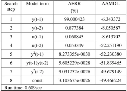
Note that the candidate model termsxi(t)xj(t)were purposely included in the candidate model (23), to check whether the new EFOR-CMSS algorithm can correctly select the significant model terms. The new EFOR-CMSS algorithm was applied to the four data sets, and the associated result is shown in Table 1, where only the first 8 selected model terms are presented. The AAMDL index in Table 1 clearly indicates that a common model structure, with 4 model terms, is preferred, and the final common-structured model was thus of the form
) ( ) 2 ( ) ( ) 1 ( ) ( ) 2 ( ) ( ) 1 ( ) ( )
(t 1 c y t 2 c y t 3 c u t 4 c u t e t
Table 1. Identification result for the mass-spring-damper system given by (22), using the EFOR-CMSS algorithm.
Search step
Model term AERR
(%)
AAMDL
1 y(t-1) 99.000423 -6.343372 2 y(t-2) 0.877384 -8.050587 3 u(t-1) 0.068845 -8.613702 4 u(t-2) 0.053349 -52.251190 5 y2(t-1) 8.273355e-0030 -52.230380
6 y(t-1)y(t-2) 5.605229e-0028 -51.839465 7 y2(t-2) 9.031232e-0026 -49.679149
8 const 3.103675e-0026 -49.466224 Run time: 0.609sec
Table 2. Parameter estimates for the selected model terms for the mass-spring-damper system given by (22).
Model term
Parameter estimates
c=2 c=10 c=20 c=40
y(t-1) 1.970306 1.895329 1.809675 1.662142 y(t-2) -0.980199 -0.904838 -0.818731 -0.670375 u(t-1) 4.962667e-005 4.833333e-005 4.679167e-005 4.395833e-005 u(t-2) 4.922973e-005 4.675501e-005 4.376735e-005 3.837817e-005
where the parametersθm(m=1,2,3,4) were viewed as a function of the adjustable coefficient c. The parameter estimates for the three model terms in (24), about the four data sets, are shown in Table 2. Assume that the parameterθmcan be fitted using the adjustable coefficient c, with a polynomial of order 3 below
3 3 , 2 2 , 1 , 0 , )
(c m m c m c m c
m β β β β
θ = + + + , m=1,2,3,4, (25)
The parametersβm,n were directly estimated using the results in Table 2. The PDCS model for the system (22) was
) 1 ( ] 10 366667 . 1 10 919167 . 4 10 945500 . 9 990002 . 1 [ )
(t = − × −3c + × −5c2 − × −7c3 y t− y ) 2 ( ] 10 370833 . 1 10 935854 . 4 10 995458 . 9 999993 . 0
[− + × 3 − × 5 2 + × 7 3 −
+ − − − t y c c c ) 1 ( ] 10 070176 . 3 10 166668 . 4 10 666667 . 1 10 995833 . 4
[ × 5 − × 7 + × 10 2 − × 18 3 −
+ − − − − t u c c c ) 2 ( ] 10 166670 . 4 10 252084 . 1 10 329174 . 3 10 995819 . 4
[ × 5 − × 7 + × 9 2 − × 12 3 −
+ − − − − t u c c c ) (t e
[image:12.595.154.449.635.714.2]4.2 Modelling a particle damper system
A particle damper is a device with one or more cavities filled with dry granular particles of diverse shapes and small sizes. The particles can move freely and the frictions and collisions between moving particles or with a container wall will arise under the vibrating motion of the structure. These collisions exchange momentum and thus dissipate kinetic energy due to frictional and in-elastic losses. Particle dampers have the advantage of being simple in geometry, small in volume, and are applicable in extreme temperature environments. More importantly, the interactions between individual grains (and between grains and the container walls) are dissipative because of surface friction and the inelasticity of collisions. An overwhelming advantage of particle dampers is that they can operate in extreme temperature conditions when using metallic, tungsten carbide or ceramic particles. This makes particle dampers extremely applicable in areas such as gas turbines, underwater conditions and other high temperature environments. Comprehensive discussions on particle dampers can be found in the literature say in Liu et al. (2005), and Rongong and Tomlinson (2005).
Several parameters may affect the performance of a particle damper and one crucial parameter is the cavity geometry. This example concerns such a geometry design parameter: the height-to-diameter ratio: R=H/D, where H and D are the height and diameter of the particle damper respectively. Five experiments, corresponding to R=2,4,6,8,10, have been completed on a particle damper device in the Department of Mechanical Engineering, University of Sheffield, and five different data sets, have been collected. Each data set consists of 2000 data pairs of the input (applied force) and the output (acceleration) observations, sampled with a frequency f =12.8kHz. The objective is to identify a s
PDCS model, with a dependence on the design parameter R, which can be used to analyze the effect of the design parameter R on the performance of the particle damper. Four data sets, corresponding to
R=2,4,6,10, which are shown in Figure 1, were used for model identification, and one data set,
correspond to R=8 , was used to test the performance of the identified PDCS model.
Denote the system input and the output sequence using {u(t)}tN=1 and {y(t)}tN=1, respectively, with
N=2000. The predictor vector for all the common-structured models was chosen to be
T
t x t x
t) [ ( ), , ( )] ( = 1 10
x , where xk(t)= y(t−k) for k=1,…, 5, and xk(t)=u(t−k+5) for k=6, …,10.
The initial candidate common model structure for all the four data sets was chosen to be a NARX model below
) ( ) ( ) ( )
( )
(
10
1 10
0 , 10
1 0 0
0 x t x t x t e t
t y
i j i
j i j i i
i
i + +
+
=
∑
∑∑
= = =
θ θ
θ (27)
terms entered into the model), are shown in Table 3, where results for AERR and AAMDL are also presented. From Table 3, the resultant common model structure is of a simple NARX representation, which only includes linear model terms and a DC term with a small value.
The PDCS model for the particle damper system was chosen to be
) ( ) ( ) ( )
( ) (
10
1
0 R R x t e t
t
y m
m
m +
+
=
∑
= θ
θ (28)
where the parameter θm (m=0,1,…,10) depends on the design parameter R. Assume that the
parameterθmcan be fitted using R, with a polynomial function below
3 3 , 2 2 , 1 , 0 ,
)
(R m m R m R m R
m β β β β
θ = + + + , m=0,1, …, 10, (29)
The parametersβm,n can directly be estimated using the results given in Table 3. The estimated values
forβm,n, for m=0,1, …,10 and n=0,1,2,3, are presented in Table 4.
Table 3. Identification result for the particle damper system described in Example 2, using the EFOR-CMSS algorithm.
Search step
Model term
Parameter for different data sets AERR
(%)
AAMDL
R=2 R=4 R=6 R=10
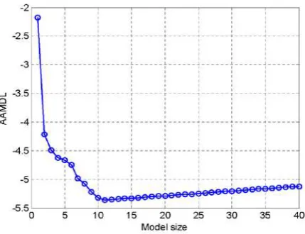
1 y(t-1) 2.1590 1.7173 1.5291 1.2342 97.7609 -2.1776 2 y(t-2) -1.7710 -0.8474 -0.4701 0.1447 2.1065 -4.2127 3 y(t-5) -0.2052 2386 0.3059 0.4939 0.0418 -4.4944 4 y(t-3) 0.8049 0.7025 0.5786 0.4173 0.0173 -4.6247 5 u(t-1) -0.3439 -0.5601 -0.6835 -0.6963 0.0046 -4.6630 6 u(t-5) -0.1668 -0.3119 -0.3875 -0.3272 0.0086 -4.7474 7 u(t-2) 1.0432 1.8016 2.2228 2.1882 0.0170 -4.9806 8 u(t-4) 0.6890 1.3032 1.6290 1.4488 0.0060 -5.2148 9 y(t-4) -0.0065 -0.8290 -0.9637 -1.3123 0.0064 -5.0786 10 u(t-3) -1.2214 -2.2329 -2.7811 -2.6139 0.0041 -5.3216 11 const 0.0051 0.0047 0.0077 0.0083 0.0013 -5.3571 Run time: 2.37sec
Fig. 2. AAMDL versus the model size of common model structure models, for the four data sets, corresponding to
R=2,4,6,10, used for the particle damper system identification.
Now consider the performance of the identified PDCS model (28), whose parameters are determined by (29) and Table 4. The data set, corresponding to R=8, which has never been used in the identification procedure, was used to test the performance of the identified PDCS model. The PDCS model was simulated using the same input as in the data set corresponding to R=8, and the output from the PDCS model was then compared with the corresponding measurements. Figure 3 presents a comparison between the model predicted output and the original measurements. Note that the model
predicted output (MPO) is defined as yˆ(t)= fˆ(yˆ(t−1),,yˆ(t−5),u(t−1),,u(t−5)), implying that )
( ˆ t
Table 4. Estimates for the parametersβm,n in (29).
Model term
n m,
β
m n
0 1 2 3
const 0 0.012800 -0.006325 0.001400 -0.000081 y(t-1) 1 3.023950 -0.566579 0.114194 0.074125 y(t-2) 2 -3.615675 0.775356 -0.161981 0.007808 y(t-3) 3 0.848050 -0.000471 -0.012125 0.000786 y(t-4) 4 2.039450 -1.418113 0.219888 -0.011159 y(t-5) 5 -1.321225 0.485829 -0.120994 0.006161 u(t-1) 6 -0.023800 -0.187875 0.014375 -0.000231 u(t-2) 7 -0.086050 0.662946 -0.050563 0.000701 u(t-3) 8 0.284975 -0.882169 0.065806 -0.000658 u(t-4) 9 -0.221950 0.531054 -0.038138 0.000174 u(t-5) 10 0.047050 -0.123988 0.008500 0.000016
A 2.13 1.88 1.63 1.38 1.13 2.13 1.87 1.60 1.33 1.20
V 5.30 4.67 4.05 3.43 2.80 14.8 12.9 11.1 9.20 8.30
4.3 Modelling of thermoplastic auxetic foams
Dynamic tests on a class of auxetic elastomeric foams have been carried out at the Department of Mechanical Engineering, University of Sheffield, and it has been shown from experimental results that the associated foam specimens present nonlinear behaviour that may be applicable to design nonlinear dynamic filters. Several parameters may affect the nonlinear dynamic behaviour of the material and the imposed compression ratio is one crucial factor. This example concerns two design parameters related to the imposed compression ratio: the Axial (A) and the Volume (V) of the associated materials. The objective is to identify a PDCS model, whose parameters depend on the design parameters A and
V, and which can be used to analyze the dynamic behaviour of the associated material when the design
parameter A and V change.
Ten cases, corresponding to the following values for the design parameter A and V, were considered in this example:
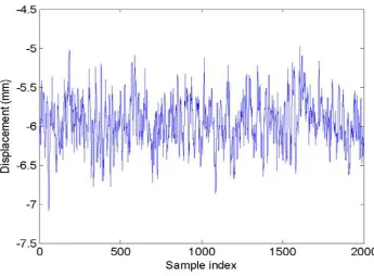
Ten different data sets, symbolized by Data01, Data02, …, Data10, corresponding to the above 10 cases, have been collected, and each data set consists of 2000 data pairs of observations for the input (displacement: mm) and the output (force: N), sampled with a frequency f =100Hz. Note that all the s
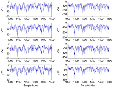
10 data sets are with the same input signal, as shown in Figure 4, but with different output signals, as shown in Figure 5, where only part of the observations are plotted for clear visualization. Eight data sets, numbered by 1,2,4,5,6,7,9, and 10, were used for model identification, and the remaining two data sets, numbered by 3 and 8, were used for the performance test of the identified PDCS model.
Denote the system input and the output sequence using {u(t)}tN=1 and
N t
t y( )} 1
{ = , respectively, with
N=2000. The predictor vector for the common model structure was chosen to be
T
t x t x
t) [ ( ), , ( )] ( = 1 4
x , withxk(t)=u(t−k+1) for k=1,2,3,4. The initial candidate common model structure was chosen to be
) ( ) ( ) ( )
( )
(
4
1 4
0 , 4
1 0 0
0 x t x t x t e t
t y
i j i
j i j i i
i
i + +
+
=
∑
∑∑
= = =
θ θ
θ (30)
This candidate model involves a total of 15 candidate model terms. Based on the candidate common model structure, the new EFOR-CMSS algorithm was applied to the 8 training data sets. The AAMDL index, shown in Figure 6, suggests that a common model structure, with 8 model terms, is preferred. The 8 selected common model terms, ranked in order of the significance, are shown in Table 5. The PDCS model for the 8 training data sets was chosen to be
) 3 ( ) , ( ) 3 ( ) 1 ( ) , ( ) 1 ( ) , ( ) ( ) , ( )
( 2 3 4 2
2
1 + − + − − + −
= AV u t AV u t AV u t u t AV u t
t
) ( ) 1 ( ) ( ) , ( ) , ( ) ( ) , ( ) 2 ( ) ,
( 6 7 8
5 AV u t− + AV u t + AV + AV u t u t− +e t
+θ θ θ θ (31)
where the parameterθm(m=1,…,8) were fitted using the following polynomial function
2 5 , 4
, 2 3 , 2 , 1 , 0 , ,
) ,
(AV m m A m V m A m AV m V
m β β β β β β
θ = + + + + + , m=1, …, 8, (32)
The parametersβm,n were directly estimated using the results given in Table 5 and the associated estimates forβm,n are shown in Table 6.
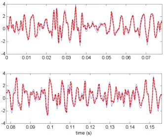
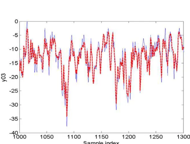
[image:18.595.119.465.417.671.2]To inspect the performance of the identified PDCS model (31), the model was simulated by choosing the same input signal as that in the two test data sets numbered by 3 and 8. The output from the PDCS model was then compared with the relevant measurements. Figures 7 and 8 present comparisons between the model outputs and the associated measurements. Note that only part of the data points are shown in Figures 7 and 8 for a close inspection. The root-mean-square-error (RMSE), defined as the root of the mean-square-error, with respect to two training data sets, was calculated to RMSE=1.71 and 6.44, respectively. Clearly, the PDCS model provides an excellent representation for the two test data sets.
Fig. 5. The output signals in the data sets numbered by 1, 2, 4, 5, 6, 7, 9, 10, for the assicated auxetic elastomeric foams.
[image:19.595.157.422.492.687.2]Table 5. Identification result for the assicated auxetic elastomeric foams described in Example 3, using the EFOR-CMSS algorithm.
Step Model term
Parameter for different data sets AERR (%) Data01 Data02 Data04 Data05 Data06 Data07 Data09 Data10
1 u2(t) -24.78 -19.10 -10.71 -10.33 -173.65 -148.65 -81.78 -66.62 88.397
2 u(t-1) 71.22 51.28 33.09 25.26 477.51 426.92 229.47 196.34 10.042 3 u(t-1)u(t-3) -0.35 0.43 -0.73 0.67 3.53 1.43 1.49 0.66 0.117 4 u2(t-3) 0.52 -0.06 0.35 -0.31 1.80 2.18 0.66 0.70 0.057
[image:20.595.135.457.310.460.2]5 u(t-2) 1.43 -0.50 -2.78 -0.19 37.94 30.22 13.51 8.64 0.025 6 u(t) -168.66 -129.39 -77.67 -67.08 -1187.99 -1016.74 -559.00 -454.19 0.015 7 const -234.68 -194.87 -118.63 -101.74 -1701.85 -1415.05 -801.24 -632.16 0.025 8 u(t)u(t-1) 14.63 10.60 6.23 5.53 100.55 88.73 47.78 40.04 0.083 Run time: 2.53sec
Table 6. Estimates for the parametersβm,n in (32).
m n
0 1 2 3 4 5
1 -14.05 20.09 -30.01 292.02 -161.80 16.52 2 47.98 -72.58 10.23 -1172.89 649.59 -67.22 3 1.81 -2.29 0.05 29.88 -16.05 1.72 4 -0.28 0.18 -0.03 -20.62 11.29 -1.19 5 16.35 -22.45 -0.70 -80.71 47.70 -4.83 6 -51.41 78.40 -20.05 1955.65 -1074.11 109.58 7 75.10 -92.45 -27.90 1688.76 -896.05 88.65 8 12.31 -17.74 1.90 -230.03 127.98 -13.21
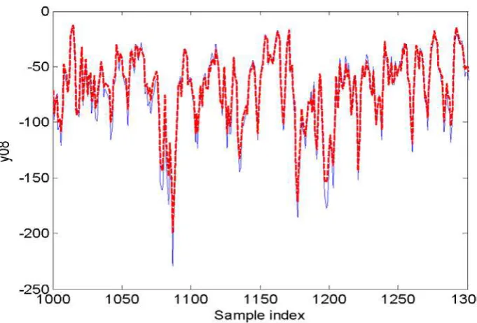
[image:20.595.133.450.458.698.2]Fig. 8. A comparison between the model predicted output from the identified PDCS model (31) and the corresponding measurements in Data08, for the assicated auxetic elastomeric foams. The thin solid line indicates the measurements, and the thick dashed line indicates the model predicted output.
5. Conclusions
Acknowledgements
The authors gratefully acknowledge that this work was supported by EPSRC(UK). The authors also gratefully acknowledge the help from J. Rongong and F. Scarpa in the data collection for the particle damper and auxetic foams respectively.
Appendix—Some abbreviations
AAMDL: average
approximate minimum description length.AERR: average error ratio reduction.
AMDL: approximate minimum description length.
CMSS: common model structure selection.
EFOR: extended forward orthogonal regression.
EPD:
external-parameter-dependent.ERR: error ratio reduction.
FOR: forward orthogonal regression.
IPD: internal-parameter-dependent. MDL: minimum description length. OLS: orthogonal least squares.
PDCS: parameter-dependent common-structured (model).
References
A. Antoniadis, I. Gijbels, G. Gregoire, “Model selection using wavelet decomposition and applications,” Biometrika, 84(4), pp. 751-763, 1997.
C. S. Berger, “Linear Splines with Adaptive Mesh Sizes for Modeling Nonlinear Dynamic-Systems,”
IEE Proc.-Control Theory Appl., 141(5), pp. 277-284, 1994.
S. A. Billings and W. S. F. Voon, “Piecewise linear identification of non-linear systems,” Int. J.
Control, 46(1), pp.215-235, 1987.
S. A. Billings, S. Chen, and M. J. Korenberg, “Identification of MIMO non-linear systems suing a forward regression orthogonal estimator,” Int. J. Control, 49(6), pp.2157-2189, 1989.
S. A. Billings and H. L. Wei, “The wavelet-NARMAX representation: A hybrid model structure combining polynomial models with multiresolution wavelet decompositions,” Int. J. Syst. Sci., 36(3), pp. 137-152, 2005.
S. Chen and S. A. Billings, “Representations of non-linear systems - the NARMAX model,” Int. J.
Control, 49(3), pp. 1013-1032, 1989.
non-S. Chen, non-S. A. Billings, C. F. N. Cowan, and P. M. Grant, “Practical identification of NARMAX models using radial basis functions,” Int. J. Control, 52(6), pp. 1327-1350, 1990.
S. Chen, X. Hong, C. J. Harris, and X. X. Wang, “Identification of nonlinear systems using generalized kernel models,” IEEE Trans. Control Syst.Technol., 13(3), pp. 401-411, 2005. C. J. Harris, X. Hong, and Q. Gan, Adaptive Modelling, Estimation and Fusion from Data: A
Neurofuzzy Approach. Berlin: Springer-Verlag, 2002.
J. A. Rongong and G. R. Tomlinson, “Amplitude dependent behaviour in the application of particle dampers to vibrating structures,” In the Proceedings of the 46th AIAA/ASME/ASCE/AHS/ASC
Structures, Structural Dynamics & Materials Conference, Art No.: AIAA 2005-2327, 18-21
April 2005, Austin, Texas, USA.
T. Kavli, “Asmod - an algorithm for adaptive spline modeling of observation data,” Int. J. Control, 58(4), pp. 947-967, 1993.
I. J. Leontaritis and S. A. Billings, “Input-output parametric models for non-linear systems, part I: deterministic non-linear systems,” Int. J. Control, 41, pp. 303-344, 1985.
G. P. Liu, Nonlinear Identification and Control: A Neural Network Approach. Berlin: Springer-Verlag, 2001.
W. Liu, G. R. Tomlinson, and J. A. Rongong, “The dynamic characterisation of disk geometry particle dampers,” J Sound Vibr., 280, pp. 849-861, 2005.
R. K. Pearson, Discrete-Time Dynamic Models. Oxford: Oxford University Press, 1999.
J. Rissanen, “A universal prior for integers and estimation by minimum description length,” Ann. Stat., 11, pp. 416-431, 1983.
N. Saito, “Simultaneous noise suppression and signal compression using a library of orthonormal bases and the minimum description length criterion,” In Wavelet in Geophysics, Foufoula-Georgiou, E. and Kumar, P., Eds, New York: Academic, pp. 299-324, 1994.
H. L. Wei and S. A. Billings, “Feature subset selection and ranking for data dimensionality reduction,” Accepted by IEEE Trans. Pattern Anal. Machine Intell., 2006.
H. L. Wei, S. A. Billings, and M. A. Balikhin, “Wavelet based nonparametric NARX models for nonlinear input-output system identification,” Accepted by Int. J. Syst. Sci., 2006.