Electrokinetic manipulation of micro to nano-sized objects for microfluidic application

Full text

(1)Electrokinetic manipulation of micro to nano-sized objects for microfluidic application. Thesis submitted in accordance with the requirements of The University of Liverpool for the degree of Doctor in Philosophy. By. Aleksandr Chichenkov. Department of Electrical Engineering & Electronics July 2013.

(2) Abstract. This thesis describes experimental and numerical investigations of various electrokinetic techniques on fluorescent particles, bacteria and protein motors. The aim of this work is to extend the knowledge on the object manipulation, which is an essential part of a practical microfluidic device. The dissertation consists of three major sections that contain novel approaches to object manipulation using electric fields. The effect of dielectrophoretic force on fluorescent particles is analysed first. Using an experimental setup with a controlled switch for the input signal, the theoretical framework for amplitude modulated responce of dielectrophoretic force is developed. Also presented is the image processing software for quantitative particle motion analysis. Another analysis of various electrokinetic techniques (dielectrophoresis, AC electroosmosis, AC electrothermal flow and electrophoresis) was carried out on Pseudomonas Fluorescence bacteria in a solution that supports its growth. These bacteria usually live in geometrically restricted spaces and so spatially confined transparent channels were created to mimic their natural environment. It was noted that in these conditions the motile bacteria do not experience the effect of dielectrophoretic force. The minimum frequency that can be applied to the solution without forming bubbles is too high to distinguish AC electroosmotic effect. Using the numerical simulation, however, the experimental setup that utilises the observed effect of electrophoresis and AC electrothermal flow is designed. The final study was carried out on protein molecular motors. The novel experimental setup to investigate the effect of the electric field on the actin filament motility on five different surfaces, covered with myosin II motors, was developed. The application of higher external electric fields resulted in different velocity increases on different surfaces. Using the numerical simulation, this difference is quantitatively explained by the variation of the number of motors on surfaces. Also presented is a novel method that enables determining the forces exerted by the population of active and resistive motors without the need of expensive equipment.. i.

(3) Acknowledgements. I would like to thank Dr. David Bakewell for giving me the opportunity to start this PhD with his advice, support and friendship. I would also like to thank Prof. Dan Nicolau for giving me the opportunity to work on an exciting multi-million EU project and introducing me to the world of molecular motors. A very special thank you goes to Dr. Harm van Zalinge, who took over the role of a primary supervisor for his tremendous support, wisdom and guiding. Many thanks to my friends from the work group: Jenny, Miguel, Laurence, Ben, Serban, Marie! Thank you guys, it’s been quite a trip! I would like to express my gratitude to the department of Electrical Engineering and Electronics for the financial support. Finally I would like to thank my family for their support and faith in me.. ii.

(4) Publications Journal Publications: D.J. Bakewell and A. Chichenkov "Fourier-Bessel Series Modelling of Dielectrophoretic Bionanoparticle Transport: Principles and Applications". IEEE Transactions on Nanobioscience (vol 11 issue 1 2012, pp 79-86) D.J. Bakewell and A. Chichenkov "Quantifying dielectrophoretic nanoparticle response to amplitude modulated input signal" (vol 45, 365402, 2012). Journal of Physics D-Applied Physics, 2012. 45(49). Chichenkov A, Ramsey L C, Van Zalinge H, Aveyard J, Persson M, Mansson A, Nicolau D V. Estimation of the force generated in the acto-myosin system through electric field modulation of motility and stochastic simulation. In preparation (2013).. Conference Publications: D.J. Bakewell, A. Chichenkov, N.A. Yunus "Models of Nanoparticle Transport in Dielectrophoretic Microdevices: Prediction, Parameter Estimation and Other Applications." IEEE EMBS Conference on Biomedical Engineering & Sciences (IECBES 2010). iii.

(5) Table of Contents Chapter I: Introduction ............................................................................................................ 1 1.1 Fluid manipulation techniques ...................................................................................... 3 1.2 Detection techniques..................................................................................................... 6 1.3 Object manipulation using electric fields....................................................................... 7 1.4 Applications.................................................................................................................... 9 1.5 Thesis outline and authors contribution......................................................................11 Chapter II: Theory. Forces acting on objects in the electric field ..........................................14 2.1 Electrophoresis ............................................................................................................15 2.2 Dielectrophoresis .........................................................................................................16 2.2.1 Dielectric spheres in an electric field ....................................................................17 2.2.2 Frequency dependent behaviour of DEP force.....................................................21 2.2.3 DEP of non-spherical particles ..............................................................................23 2.2.4 DEP of rod-shaped bacteria ..................................................................................25 2.3 AC Electroosmosis........................................................................................................28 2.4 AC electrothermal fluid flow........................................................................................31 2.4.1 The force on the fluid in electric field due to Joule heating .................................32 Chapter III: Fabrication and other related technologies........................................................36 3.1 Electrode fabrication using laser ablation ...................................................................37 3.2 PDMS fabrication .........................................................................................................41 Chapter IV: Amplitude Modulated Dielectrophoresis ...........................................................44 4.1 Introduction .................................................................................................................45 4.2 System model..............................................................................................................47 4.3 Concepts and Parameters............................................................................................49 4.4 Normalised Amplitude AN ............................................................................................52 4.5 Experimental materials and methods..........................................................................53 4.6 Number of particles and fluorescent intensity relationship........................................56 4.7 Effect of varying the switching frequency ...................................................................58 4.8 Effect of varying the duty cycle....................................................................................61 4.9 Conclusion....................................................................................................................62 Chapter V: The Behaviour of the Bacteria in Channels with External Forces ........................64 5.1 Introduction .................................................................................................................65 iv.

(6) 5.2 The bacterial structure and growth .............................................................................66 5.3 Bacteria in channels .....................................................................................................68 5.3.1 Overview ...............................................................................................................68 5.3.2 Bacterial Growth Conditions.................................................................................71 5.2.3 Experimental procedure .......................................................................................72 5.4 Details of the numerical simulation.............................................................................74 5.4.1 Equations used in the simulation..........................................................................76 5.5 Results of the electric field effect on the bacteria.......................................................82 5.5.1 Effect of constant electric field on the bacteria....................................................82 5.5.2 DEP effect on the bacteria ....................................................................................84 5.5.3 ACEO effect on the bacteria..................................................................................87 5.5.4 ACET effect on the bacteria ..................................................................................89 5.5.5 Proposed design for a channel geometry .............................................................94 5.6 Conclusion....................................................................................................................97 Chapter VI: The Effect of Electric Field on the Behaviour of Molecular Motors .................100 6.1 Introduction ...............................................................................................................101 6.2 The molecular motors................................................................................................102 6.2.1 Types of motility assays ......................................................................................103 6.2.2 Operating principle of molecular motors ...........................................................105 6.2.3 Processivity of molecular motors........................................................................107 6.2.4 Duty cycle of molecular motors ..........................................................................109 6.2.5 Applications of molecular motors.......................................................................111 6.3 Detecting the protein motors on the surface ............................................................111 6.4 Guiding the molecular motors ...................................................................................113 6.5 In Vitro motility in the electric field ...........................................................................116 6.5.1 Materials and methods .......................................................................................116 6.5.4 Effect of the electric field on motility .................................................................121 6.6 Model description......................................................................................................123 6.7 Simulated results .......................................................................................................129 6.8 Conclusion..................................................................................................................136 Chapter VII: Conclusion........................................................................................................139 Appendix ..............................................................................................................................143 References ...........................................................................................................................147. v.

(7) Chapter I: Introduction. 1|Page.

(8) The development of the electronic circuits and consequently the silicon fabrication technology in 20th century has had an enormous impact in various fields of science. Currently one the most developed and explored aspect of silicon fabrication from the commercial point of view is the integrated circuit based devices [1, 2]. Over the last few decades, however, an enormous interest in the alternative exploitation of the fabrication technology has been witnessed with a particular interest in microsystems for biological and chemical analysis. As a result a number of concepts have been developed including microelectromechanical system (MEMS), microfluidic devices, microarrays, etc [3, 4]. Another concept that is aimed towards developing a practical microfluidic device is a micro- total analysis system (µTAS) or a lab-on-a-chip technology where a number of functions such as separation, concentration and detection are performed in a single device. The aim of this technology is to shrink the conventional laboratory based equipment into a chip through the integration of functional units like pumping, concentration, separation and detection systems. A number of theoretical models and academic proof-of-concept studies have demonstrated the advantages of lab-on-achip system over laboratory tests [5-9]. The common feature of microfluidic devices is the handling and manipulation of small amounts of fluid usually in micro and nano-liters or even in pico-liter range. These devices can have virtually any design however the system has a series of generic components: an inlet mechanism i.e. the method of introducing the reagents and samples (this can simply be a reservoir on the chip where the sample in the solution is pipetted into), a mechanism to move and mix the fluids on the chip and detection mechanism depending on the desired application of the device [10]. 2|Page.

(9) 1.1 Fluid manipulation techniques. There is currently a wide range of techniques (a categorised list is presented in figure 1.1) to produce fluid flow that can be used as means to move the sample within the chip and/or mix the fluids.. Figure 1.1. A categorised list of currently used fluid manipulation techniques. The figure was reprinted from [11]. The selection of the fluid pumping technique depends on the desired application. These may vary over a wide range: from low power, low flow-rate to high flow-rate, high pressure pumping. The techniques for micropuming can be broadly divided into 2 categories:. 3|Page.

(10) 1. Mechanical displacement micropumps - defined as "those that exert oscillatory or rotational pressure forces on the working fluid through a moving solid-fluid (vibrating diaphragm, peristaltic, rotary pumps), or fluidfluid boundary (ferrofluid, phase change, gas permeation pumps)" [11]. 2. Electro- and magneto-kinetic micropumps - defined as "those that provide a direct energy transfer to pumping power and generate constant/steady flows due. to. the. continuous. addition. of. energy. (electroosmotic,. electrohydrodynamic, magnetohydrodynamic, electrowetting, etc.)"[11]. These caterogires can be further sub-divided according to actuation principles. A detailed analysis of the techniques as well as their applications can be found in literature [12, 13]. However, only some of these techniques are used to generate the fluid flow in microfluidic devices. Namely these techniques are [14]: Gas boundary displacement - most commonly an external syringe or vacuum pump is connected to a microfluidic channel via an inlet/outlet. The pressure is applied to a syringe that contains either liquid of gas and is connected to a channel. As a result the motion of fluid is produced. Similarly, the liquid can be dragged from the reservoir using a vacuum pump by removing the gas from the channel. Membrane actuated displacement - This system consists of a closed chamber with valves and a membrane made out of specialised material. Upon application of external source, the material undergoes the change which results in a force production. In case of thermal actuation, the volume of the material expands or stress is produced in response to external heat. Alternatively piezoelectric material can be used for membrane as this material undergoes the mechanical stress in presence of 4|Page.

(11) the applied electric potential. Other types of membrane actuated displacement include electrostatic and electromagnetic mechanisms. Ferrofluidics displacement - In this system ferrofluid is separated from the working fluid with an oil plug. The diagram of a simple ferrofluidic pump is shown in figure 1.2. The motion of the magnet produces the fluid flow from the inlet to outlet.. Figure 1.2. A schematic diagram of a ferrofluidic piston pump. The figure was reprinted from [15]. Other methods include the use of capillary force [16, 17] or gas bubbles [18] to produce the motion inside the channels. Alternatively to the techniques discussed so far, the pumping system can be integrated onto the chip itself. Some of these methods include elecotrhydrodynamic, magnetohydrodynamic and electroosmotic pumps. According to a comparison of various pumping techniques in a recent comprehensive review [11], piezoelectric diaphragm pumps, induction- and injection-type electrohydrodynamic and electroosmotic pumps produce high flow. 5|Page.

(12) rates per unit area. In addition electroosmotic pumps offer great miniaturisation potential, which makes it favourable technique for microfluidic application.. 1.2 Detection techniques. One of the detection techniques that is used in the microfluidic and lab-on-a-chip system is the optical detection. It is a very common detection method due to the ease of implementation [19]. Out of the number of optical detection methods, the fluorescence detection is the most popular method for the microfluidic devices due to the excellent sensitivity which is often required because of the small sample volume involved. In fluorescence microscopy the specimen is illuminated by a light of a specific wavelength which is absorbed by fluorophores causing them to emit light of a different wavelength (i.e. of a different colour) than the absorbed light. The illumination and emission light is separated by the use of a spectral emission filter. Alternatively, charge couple device (CCD) cameras [20, 21] and photomultiplier tubes [22] (PMT) can also be used to detect the emitted fluorescent light. The equipment, required for the fluorescence detection is, however, very large, which constrains the portability of microfluidic devices. In addition only the natively fluorescent or are amendable to labelling analytes can be detected [23]. Another commonly used optical detection method is the ultraviolet-visible light (UV-Vis) absorbance detection. In this system when the emitted light passes through a sample, the molecules within the sample absorb the energy to move the electrons to 6|Page.

(13) a different energy state. The detection is made according to the wavelength, required to promote the electron to a different state. The signal of such system is pathlength dependent and the small scale of the microfluidic devices severely minimises the sensitivity of the measurements on the chip [14]. In recent studies, the photothermal absorbance detection technique was presented [23, 24]. This technique relies on the physical changes (refractive index, viscosity and conductivity) in the solution that take place when an analyte absorbs the light of the excitation beam. Other optical detection methods include surface plasmon resonance, where the frequency of the light photons matches the natural frequency of the surface electron oscillation, which is sensitive to the surface absorbed molecules and Raman spectroscopy. For microfluidic system, however, surface enhanced Raman spectroscopy [25, 26] is generally used due to the sensitivity limitation of the conventional analysis [27]. Another mechanism for detection is electrochemical detection. It has the potential to be compact and fully integrated as the signal is detected using the electrodes [28, 29]. The system can be used to detect the molecules that undergo oxidation or perform conductivity measurements [30, 31]. Recently mass spectrometry has been used in microfluidic systems for ultrasensitive analysis of microscale samples [32].. 1.3 Object manipulation using electric fields. One of the main challenges for a practical application of a lab-on-a-chip device is to be able to manipulate objects on small scales. The manipulation mechanism has to be 7|Page.

(14) compatible with the miniaturised portable system, highly reliable and easy to maintain. Among the large number of manipulation methods reported in literature [33], electrokinetic techniques are currently most favourable. The electrokinetic techniques can be separated into two categories according to the type of signal that is applied: AC and DC electrokinetics. The list of the forces produced by the electric field that can be exerted on objects is given in table 1.1 Table 1.1 A summary of electrokinetic forces that can be exerted on objects in aqueous solution due to external electric field and the origin of the effect.. Force. DC. AC. Electrophoresis. . Dielectrophoresis. . . Induced dipole and non-uniform field. Electroosmosis. ×. . . Charge in double layer and tangential field. . . Electrothermal flow. Origin (Interaction of) Charge and the electric field. Gradients in permittivity and conductivity of the fluid and the electric field. A large number of studies have been carried out for both DC and AC electrokinetic effects. In the context of manipulation for lab-on-a-chip application, however, the preference has been given to AC effects for a number of reasons, such as the fact that the alternating fields significantly reduce electrolysis, prevent bubble formation, suppress electrochemical reaction and maintain the pH level at the interface between the electrode surface and the electrolyte [34, 35]. In a system with alternating electric fields, low voltages are generally applied over closely spaced microfabricated electrodes producing large electric fields. These fields are capable of directly moving the objects through an induced dipole and field interaction. i.e.. dielectrophoresis. (DEP),. traveling. wave. dielectrophoresis, 8|Page.

(15) electrorotation and electroorientation, or indirectly by producing fluid motion via electroosmosis or electrothermal flow, which drags the object in the direction of the induced flow.. 1.4 Applications. One of the most highly developed applications of microfluidic devices is their use for screening of protein crystallisation conditions (such as pH, ionic strength and composition and concentration) [36-38], as these devices offer a potential to screen a large number of conditions, minimise the damage to crystals and separate the nucleation and growth [10]. Considering the small sample volumes and no need for an expert to operate them, these devices look very appealing for diagnostics [39-43]. Low weights makes it portable and so it can be used directly at sides were samples are taken which results in the short time frames for the results to be obtained with less chance of contamination. The mass production would also enable low cost which is particularly important for the third world countries where buying the expensive specialised equipment for laboratory tests may not be possible. A particularly important contribution in the development of microfluidic devices is the polydimethylsiloxane (PDMS) material. It is a transparent elastomer with low toxicity and high permeability to dioxygen and carbon dioxide. In cell biology PDMS microfluidic system can be used in a wide range of studies such as. 9|Page.

(16) cytoskeleton [44, 45], the contents of cell (down to single-cell level) [46-49] as well as separation of motile and non-motile cells (e.g. sperm [50]). In addition, PDMS-based microfluidic devices can be used to perform a range of studies on the bacteria. For example, the studies of macro-scale flow of bacterial biofilms (groups of microorganisms in which cells stick to each other on the surface) are conventionally conducted in a low-throughput environment, generally require large volumes of sample and do not allow spatial and temporal control of biofilm community formation [51]. The mentioned devices help to overcome the problems associated with these studies. Additional benefits of microfluidic based bacterial biofilms investigation are the control of the hydrodynamic conditions, real time monitoring and the ability to establish stable chemical gradients [52-55]. These devices are also used for other applications, such as exploring the bacterial microenvironments [56] as well as the separation [57-60] and detection [61-67] of the bacteria. The integration of protein molecular motors into a microfluidic system is another line of research which has been heavily investigated by means of the in vitro motility assay [68-73]. These motors convert chemical energy (ATP) into mechanical work in a very energy efficient manner and are naturally “designed” for cargo transportation without the need of induced fluid flow. Moreover the proteins that are sliding above the motor covered surface in a typical experiment are extremely small (the radius of actin filament and microtubule are only few nanometers) which is beneficial when building devices of micron and sub-micron scale.. 10 | P a g e.

(17) 1.5 Thesis outline and authors contribution. The aim of this thesis is to explore the capabilities of currently used electrokinetic techniques for a practical microfluidic device. Through a set of experiments aided by numerical simulations a theoretical framework has been developed that could be of critical importance when designing a device for bacterial analysis and/or uses protein molecular motors. The complete dissertation consists of the following major sections: chapter I serves as an introduction to the background and the motivation of this work. The theoretical background of the electrokinetic techniques used for the object manipulation is presented in chapter II. Small distance between electrodes enables application of high electric fields at low voltages. Using the laser ablation technique the electrodes can be fabricated as shown in chapter III. Also presented is the microfluidic channel fabrication procedure and surface topography imaging using the atomic force microscope. One of the commonly used techniques for object manipulation on microscale is dielectrophoresis. The force, associated with this phenomenon depends on the properties of both particle and the medium. In chapter IV a mechanism for a novel object characterisation using amplitude modulated dielectrophoresis is developed. Authors Contribution to the amplitude modulated dielectrophoresis chapter is the following: I have designed and performed a range of experiments using the squarewave modulated input signal applied to castellated electrodes as well as quantitatively analysed the effect of changing the frequency and duty cycle of the 11 | P a g e.

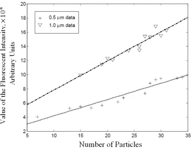
(18) square wave. Developed an image processing tool using Matlab software for fluorescence intensity (quantitative) analysis of the cyclic collection-diffusion behaviour. Performed an experiment to determine the relationship between the fluorescence intensity and particle number for 512 nm and 1 µm particles. A systematic study of various electrokinetic techniques is presented in chapter V. The techniques were used to manipulate the Pseudomonas Fluorescence bacteria in microfluidic channels. These spatially restricted channels resemble the geometrically confined natural habitat of the bacteria. Authors contribution to this chapter included design of experimental setup for AC and DC electric field manipulation. More specifically a fabrication of the "needle" device for DC analysis as well as performing the experiments on the bacteria in such device. Experimental investigation of DEP and ACEO effect on motile and nonmotile bacteria. Fabrication of the gold ablated electrodes and PDMS channel (as discussed in the fabrication chapter) for ACEO and ACET analysis. I have also developed numerical simulations using Comsol software to: . Minimise the experimental setup used for DC analysis to dimensions typical to microfluidic system. . Compare the experimentally observed motion of the bacteria influenced by ACET and the simulation produced streamlines. . Design the channel geometry that allows producing a unidirectional flow using the PDMS topography. 12 | P a g e.

(19) In addition the heat map of the bacteria motion inside the Venice waterways was produced using the Matlab software. In chapter VI the experimental setup to manipulate negatively charged protein molecular motors is developed. This setup allows the application of relatively large electric fields without producing bubbles and free radicals that are harmful for the proteins. Also presented is the numerical simulation that uses the experimentally obtained results to gain more insight on the protein-surface and motor-filament interaction. Authors contribution to this chapter was the development of the numerical simulation that allows calculating the number of motors on the surface as well as determine the active and resistive force of motors that interact with the filament. The author has also developed a method of calculating the number of lever arms that can interact with the filament for a given number of motors on the surface. I have also assisted on performing the electrical motility experiments and determining the ratio of active and inactive motors.. 13 | P a g e.

(20) Chapter II: Theory. Forces acting on objects in the electric field. This chapter gives a theoretical background to various electrokinetic techniques that are used to manipulate objects suspended in aqueous solutions. More specific these manipulation methods are electrophoresis, dielectrophoresis, AC elektroosmosis and AC electrothermal flow. 14 | P a g e.

(21) 2.1 Electrophoresis. Electrophoresis is commonly referred to as the steady transition of a particle under the influence of a spatially uniform electric field [74-76]. This phenomenon was first described by Reuss in a paper published in 1809 [77]. Reuss has noticed that the application of the electric field caused clay particles suspended in water to migrate. However, it would take almost 100 years to explain the underlying principles of the phenomenon [78]. It is currently known that the electrokinetic properties of a particle in suspension are governed by the electric charge distribution in the double layer that surrounds the particle [79, 80]. The formation of this double layer takes place when a solid particle that carries a surface charge suspended in a liquid becomes surrounded by counter-ions (of opposite charge to that of the surface of the particle). As the particles move through the solution, the plane beyond which the counter-ions do not migrate along with the particle is known as the slipping plane. The electric potential at the slipping plane is known as the zeta potential . The term that describes the rate of particle motion under the electric field is the electrophoretic mobility, µ. =. E. where. ,. (2.1) is the velocity and E is the electric field strength. The electrophoretic. mobility is also dependent on zeta potential. Assuming that the thickness of the double layer is negligible in comparison with the particle diameter, the expression for the electrophoretic mobility is given by equation 2.2. 15 | P a g e.

(22) = Here. . is the permittivity of free space,. of the suspending medium, respectively.. (2.2) and. are the permittivity and viscosity. is the zeta potential of the suspended. particle. Electrophoresis is currently a common technique for molecule separation. Few of the many applications include DNA, protein, antibiotics and vaccine analysis. Various types of electrophoretic setups are currently used, however most commonly gel medium (Electrofocusing gels, DNA agros gels, DNA denaturing polyacrylamide gels, etc.) is used for the separation.. 2.2 Dielectrophoresis. The term dielectrophoresis commonly refers to a micro to nanoscale manipulation technique which takes place due to the interaction of a non-uniform electric field with the induced dipole of an object, suspended in the solution. Pohl [81] was one of the first to recognise and explore the applications of the force that this system experiences. This force strongly depends on the gradient of the electric field, thus on the distance between electrodes. His early work to observe the effect of DEP generally involved needles, wires and flat surfaces to generate inhomogeneous electric fields [81, 82], however, the forces generated in these studies were relatively small and presented results received little attention. With the advance of microfabrication techniques, larger electric fields could be produced, re-igniting the interest in this area. Currently DEP theory is well established (the summary can be 16 | P a g e.

(23) seen in a recent review by one of the pioneers in the area [83]) and a number of analytical and numerical approaches have been presented [84-88]. DEP force is routinely used in a whole range of applications presented in a comprehensive review [83] with over 950 journal papers published in the last 5 years. Different electrode geometries are used to investigate conventional dielectrophoretic behaviour [89-94] and more recently insulator-based [95, 96] and contactless techniques [97] have been developed.. 2.2.1 Dielectric spheres in an electric field. In order to explain how force, acting on an object in a non-uniform electric field is produced, it is essential to analyse the charge distribution at the interface between two materials of different conductivity and/or permittivity. Conductivity is a measure of the ease with which charge can move through a material, while permittivity describes the amount of electrical energy (or charge accumulation at the interface) stored in a material. In a DEP system, these two materials are a particle (which in reality can be a latex bead, a cell, a virus, bacteria or a protein molecule) and an aqueous solution [35]. Dielectric materials ideally have no free charge and all electrons are bound to the nearest atom or molecule. They exist in two types: polar dielectrics and non-polar ones. When the electric field is applied, bound charges are forced to move slightly with positive and negative charges moving in opposite directions. The charge distribution around a particle can be described by introducing a concept of Polarisability, which is a measure of the ability of a material to respond to a field 17 | P a g e.

(24) (polarise) and produce charge at the interface. It can be otherwise described as the ability of a material to acquire a dipole through the action of an external electric field. There are three basic molecular polarisation mechanisms that can occur when an external electric field is applied to a homogeneous dielectric: Electronic, atomic and orientation (or dipolar). Electronic polarisation is present in both polar and non-polar materials when the electric field acts on electrons and nucleus of an atom, distorting the electron orbitals such that their average position does not coincide with nucleus. Atomic polarisation takes place within the material when differently charged ions are displaced. Polar dielectrics contain atoms (or molecules) that possess a permanent dipole moment (randomly oriented). Alignment of these permanent dipoles is called orientational polarisation. Real systems are often heterogeneous (i.e. consist of a number of different dielectrics each with its properties). For such systems, when an electric field is applied, surface charge accumulates at the interface between different dielectrics. This is referred to as interfacial or Maxwell-Wagner polarisation. In a dielectrophoretic system that is used in these studies, when an electric field is applied, the interface between the particle and the suspending medium undergoes the Maxwell-Wagner polarisation.. 18 | P a g e.

(25) Figure 2.1. Effect of uniform electric field on uncharged particle. The polarisability of particle is greater (a) and less (b) than that of the suspending medium. Figure was adapted from [35]. Consider the case, where a spherical particle is suspended in an electrolyte and subjected to a uniform electric field. A charged particle will experience a net force towards the electrode of opposite polarity through electrostatic force or Coulomb interaction. A neutral particle will become polarised as a result of the electric field, but will not experience any net force. Depending on the polarisability of the particle and medium, the net induced dipole can have different direction. When the polarisability of the particle is greater than the electrolyte, there are more charges just inside the interface rather than outside (figure 2.1a). The difference in charge density gives rise to an effective (induced) dipole across the particle aligned with the field. For a medium with polarisable larger than that of a particle, the direction of induced dipole is reversed (figure 2.1b). Equal polarisability of a particle and medium results in zero effective dipole. 19 | P a g e.

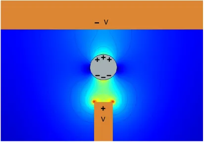
(26) Figure 2.2. Simulated non-uniform electric field displays different field strength acting on the same particle. This imbalance leads to a force – dielectrophoretic force.. When placed in a non-uniform DC electric field a charged particle will still experience the force toward the electrode of opposite polarity. However a neutral particle will experience a force, moving it away or towards the regions of high electric field intensity. The reason for this force is the following: charge distribution at the interface may be considered of equal amounts towards +V and –V as shown in figure 2.1. However the field line density is different which leads to different field strengths on one side of the particle than the other (illustrated in figure 2.2) and as a result an imbalance of forces on the induced dipole, leading to particle movement. This effect is called dielectrophoresis. The formation and/or orientation of a dipole does not occur instantaneously. By reversing the polarity of electrodes in figure 2.2, the resulting charge distribution of a 20 | P a g e.

(27) sphere would also change. This redistribution takes some time and clearly if the frequency, at which the polarity of electrodes is reversed, is continuously increased at a certain point the motion of the charge will no longer be able to keep up with the pace of the field and polarisation no longer occurs.. 2.2.2 Frequency dependent behaviour of DEP force. The complex permittivity describes the frequency dependent response of the dielectric particle to an applied electric field [98] and is given by ̃=. where. −. dielectric,. (2.3). ,. is absolute permittivity of vacuum, is the conductivity and. is the relative permittivity of the. is the angular frequency, 2. . From the. above discussion (2.2.1) it becomes apparent that a homogeneous dielectric sphere, suspended in homogeneous dielectric medium will experience interfacial polarisation. The effective dipole moment (derived in [99]) in this case is given by. =4 here. ̃ − ̃ ̃ +2 ̃. ,. (2.4). is the permittivity of the suspending medium (i.e. fluid),. permittivity of the particle,. is the. is the radius of the particle, and E is the electric field. strength. The term in brackets is called the Clausius-Mossotti factor,. , for a. spherical particle. The force, acting on the induced dipole is further derived in [35] and the result is: 21 | P a g e.

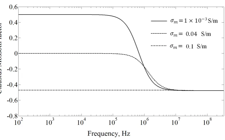
(28) = ( ∙ ∇) ,. (2.5). and the full equation of time-averaged DEP force on a spherical particle is given by ⟨. ⟩=2. Re{. }∇| | .. (2.6). The variation of magnitude and direction of the force is determined by the real part of. which depends on the conductivity and permittivity of the particle and the. surrounding medium. When analysing the particle conductivity, it is important to consider the effect that the surface charge has on the dielectric response. For example it has been noted that the latex particle (which has the bulk conductivity of the order of 10. S/m) exhibited anomalously high values of internal conductivity.. This anomaly is explained by the fact that the total particle conductivity attributed to the surface charge movement is determined using the following equation [100]: 2. =. +. where. and. ,. (2.7) are the respective particle and bulk conductivities,. surface conductivity (for a spherical latex particle radius of a sphere.. ≈ 10. S [100]) and. is the is the. The Clausius-Mossotti factor is calculated in a Matlab program (program code is similar to [100]) for a sphere with a diameter of 1 µm, conductivity of S/m, permittivity of 80. of 2.5. (. = 8.85 × 10. and three different conductivities. = 0.04. F/m), suspended in a medium with. of 1 × 10 ; 0.04 and 0.1 S/m. The. result is displayed in figure 2.3. When the real part of. is positive, the particle is. attracted to a region of high electric field and this attracting force is called positive dielectrophoresis (pDEP). At a negative value the particles are repelled from that 22 | P a g e.

(29) region experiencing negative Dielectrophoretic force (nDEP). A transition point of zero value is termed a crossover frequency. No net force is exerted on particle in this case.. Figure 2.3. Plot of real part of. as a function of frequency at different medium conductivities. 2.2.3 DEP of non-spherical particles. So far the polarisability of a sphere with a very simple internal structure has been considered. Biological particles, such as cells, viruses and bacteria have a more complex structure which is generally modelled as multi-shell system. For sphere-like biological particles concentric shells, each having its own electric properties, are used.. 23 | P a g e.

(30) Figure 2.4. (a) Schematic of a spherical particle with a single shell. (b) The frequency variation of the equivalent Clausius-Mossotti factor with = 2.01 × 10 m, = 2.0 × 10 m, = 78.5 , = 10 , = 60 , = 10 Sm , = 10 Sm , = 0.5 Sm . (a) was re-drawn and (b) re-printed from [35]. The simplest example is that of a single shell particle e.g. red blood cell is schematically shown in figure 2.4. This system has 2 different types of materials which respond differently to an external electric field. The polarisability. is given. by. =3 ̃. ̃. − ̃ +2 ̃. ,. (2.8). and the complex permittivity of the particle ̃ , is given by ̃. +2. = ̃. with. −. = .. ̃ − ̃ ̃ +2 ̃ ̃ − ̃ ̃ +2 ̃. ,. (2.9). 24 | P a g e.

(31) More shells can be adopted to mimic more complicated systems say cell membrane, nucleus and cytoplasm of animal cell. However, not all microorganisms have spherelike structure. In fact their geometry can be very diverse.. 2.2.4 DEP of rod-shaped bacteria. Throughout this work the rod-shaped bacteria and proteins were used so it is sufficient to show the DEP force, derived for a prolonged ellipsoid [101, 102] whose major axis is parallel to the electric field:. ⟨. ⟩=2. where. ,. 3. Re. and. (. =. ̃ − ̃ [ ̃ +( ̃ − ̃ )×. and. =. ln. 2. 1+ 1−. ∇| | ,. (2.10). ) are the lengths of major and minor axes.. “depolarisating factor” along the major axis. =. ]. −2 ,. is the. and is given by:. (2.11). is the particle eccentricity. 1−. .. (2.12). Using the equations 2.10-2.12 the effective Clausius Mossotti factor was calculated for a Pseudomonas putida bacteria with the conductivity of 20 mS/m [103, 104] in the media that supports the bacteria growth (more detail in section 5.3.2) with conductivity of 16.4 mS/m and distilled water with conductivity of 15.6 µS/m. It was 25 | P a g e.

(32) previously determined that as the bacteria cell dies, the effective conductivity of the cell increases and as a result selective trapping of dead and alive bacteria by dielectrophoretic force is observed [105].. Figure 2.5 The Claussius Mossoti factor, calculated for a no shell model. The dead* bacteria represents the conductivity, 5 times larger than the live bacteria cell (100 mS/m) and the simulation was performed using the value of relative permittivity of 60 (similar to a mammalian cell [106]). These values were used for illustration purpose as exact values were not available.. The no-shell system in figure 2.5 suggests that the relatively weak positive dielectrophoretic effect is present at frequencies up to tens of MHz range (Clausius Mossoti factor at these frequencies is 0.07). However, provided that the changes in the cell conductivity once the cell dies will significantly increase, stronger positive DEP effect at the same applied signal could be noted. In other studies, where the shell model has been used, it was suggested that the conductivity of the e. coli bacterial cell membrane increases by 4 orders of magnitude as the bacteria dies [107]. Assuming that the conductivity data of the bacteria, used for the experiments, is similar to the e.coli bacteria, the simulation of a 26 | P a g e.

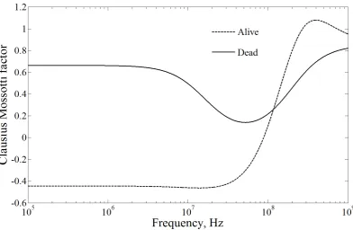
(33) two-shell model was performed as discussed in [101] and the result is shown in figure 2.6. The conductivity of medium was 16.4 mS/m and the relative permittivity of the cytoplasm, cell membrane, cell wall and the medium were 60, 10, 60 and 80 respectively.. Figure 2.6 The Clausius Mossotti factor calculated for a 2 shell model of dead and alive bacteria. See text for more details.. The two shell simulation was developed for a bacterial cell with a cytoplasm, membrane and cell wall. The values of permittivity for dead and alive cell were kept constant [108]. The conductivity values for the live bacteria were used similar to the data of e.coli [101]: 5 × 10. = 0.5 S/m,. = 10. S/m and. =. S/m. It was further assumed that as the cell dies, the conductivity of the. cytoplasm decreases (provided that the conductivity of the medium is lower). The simulation of the Clausius Mossoti factor for the dead bacteria was performed using = 3 × 10. S/m,. = 10. S/m and. = 5 × 10. S/m.. These values were used for illustration purpose and an exact model would require a 27 | P a g e.

(34) more sophisticated shell system with accurate conductivity and permittivity measurements of live and dead bacterial cell. In contrast to a no-shell model, figure 2.6 suggests a possible transition between the negative dielectrophoretic effect for a live cell to a positive dielectrophoresis for a dead one similar to the data reported in [109].. 2.3 AC Electroosmosis. As discussed for dielectrophoresis, when an electric field is applied, a double layer is formed at the interface of the particle and the suspending medium. For such a system it is also important to analyse the behaviour of the free charges at the electrode edges. When coming in contact with the free ions in fluid, (this could be electrolyte or a dielectric fluid with ionic impurities) charged electrodes attract counterions from the bulk to establish charge neutrality. As a result the density of the counterions in the solution right at the interface with the electrodes is higher than in the bulk. Helmholtz was the first to propose the concept of an electrical double layer forming between the electrode and the electrolyte [110]. In his model he assumed that all counterions are absorbed at the surface of the electrode, which can be treated as a parallel plate capacitor separated by a specific distance. Realising that the ions in the solution are mobile, Gouy and Chapman have re-designed the model where ions were treated as point charges [111, 112]. The result was a so called diffusive layer model. Stern has combined the two models, describing the double layer as two layers: the first layer contains strongly bound immobile ions and the second diffusive layer with mobile ions to which the Gouy-Chapman model applies [113]. More 28 | P a g e.

(35) details on the current understanding of the double layer can be found in literature [35, 75].. Figure 2.5. A schematic diagram representing the mechanism of AC Electroosmosis. (a) shows the charge layer around electrodes, electric field between two electrodes and it’s tangential component E t. Induced charge experiences a force Fc due to Et. (b) The interaction of Et and charge within the double layer results in fluid motion. The figure was adapted from [35].. In the case of a constant electric field, the double layer forms according to the amount of charge at the electrode surface and the free ions in the solution. For an alternating field the formation of a double layer becomes more complicated. The ions in the solution have to keep up with the charges produced on the electrodes. At a certain frequency free ions will no longer be able to respond to the oscillations of the field, resulting in the absence of the effect of electrode polarisation at high frequencies. 29 | P a g e.

(36) However, when the double layer is present, the electric field tangential to the surface of the electrode can act on the mobile ions inside the double layer moving them in the direction of the field (illustrated in figure 2.5). As a result the fluid is dragged along by the ions and this motion is termed Electroosmotic flow. The AC analogue of Electroosmosis has been demonstrated and theoretical work developed using finger electrodes [114-118]. Even though AC Electroosmosis (ACEO) is effective even at relatively large distances from electrodes (compared to DEP) it is generally restricted to a low range of frequencies and low conductivity media as shown in figure 2.6.. Figure 2.6. The velocity profile of a spherical particle observed 10 µm away from the electrodes for different media conductivities. As the conductivity increases, the magnitude of the fluid flow decreases. At high frequencies no ACEO is observed. The figure was reprinted from [117].. 30 | P a g e.

(37) The peak velocity is shifted towards higher frequencies for higher medium conductivities and no ACEO is observed at 100 kHz or higher (figure 2.6).. 2.4 AC electrothermal fluid flow. The electrokinetic technique that dominates at high frequency and in high conductivity media is electrothermal flow (ACET). It is produced by the nonuniform electric field, which causes power dissipation in the fluid – Joule heating. The amount of energy dissipated in the system is given by 1 ⟨ ⟩= ⟨ 2. where. ⟩,. (2.13). is the conductivity of the electrolyte. The produced heat (also non-uniform). diffuses through the system producing gradients in permittivity and conductivity. Consequently, a force is generated as the electric field now acts on these gradients [119]. In addition it has been shown that external light sources (e.g. observing the sample using the fluorescent microscope), at low voltages can play an important role for the resulting fluid flow [120] in the system with closely spaced electrodes. As already mentioned, ACET is efficient in a high conductivity medium, which makes it useful for manipulating biological specimen in their natural environment. This technique has a short history since it was introduced in 1990’s with the majority of studies focusing on its ability to act like a pump with functional dimension in micrometre range to induce directed motion [121-124] or mixing [125, 126] of fluids.. 31 | P a g e.

(38) 2.4.1 The force on the fluid in electric field due to Joule heating. In order to derive the force, acting on the fluid, the electric field that produces the Joule heating has to be discussed first. In the small temperature gradient (STG) approximation the electric field can be determined by solving Laplace’s equation [35]: ∇. = 0,. where +. (2.14). is the potential phasor which is given by a real and an imaginary part. =. . For a two-dimensional situation with an electrode length larger than the. width and ignoring the imaginary part [84] the electric field can be derived from = −∇ .. (2.15). For high conductivity media and high applied voltages the small temperature approximation is no longer accurate and an enhanced model that uses electrical thermal coupling and temperature dependent expression for the electrical conductivity and dynamic viscosity has recently been developed [127]. Substantial differences between the results of the enhanced model and STG were observed when the temperature increases by more than 5 oC, which was not achieved in our system. Therefore in the rest of this thesis the small temperature gradient approximation has been used. In order to find the changes in the temperature, it is necessary to solve the energy balance equation. This has been shown to reduce to a heat diffusion equation [114]:. ∇. 1 + ⟨ 2. ⟩ = 0,. (2.16). 32 | P a g e.

(39) where k is thermal conductivity. Finally, when both field and temperature profiles are determined, the force produced due to Joule heating in a non-uniform electric field can be calculated. The general expression of the electric body force is given by [35] 1 1 − | | ∇ + ∇ 2 2. = and. | |. ,. (2.17). are the charge and mass densities respectively. The right hand side consists. of Coulumb force, dielectric force and electrostriction pressure; the latter can be ignored for an incompressible fluid. When relative changes in permittivity and conductivity are small, the changes in charge density and electric field are also small and the electric field can be expressed as a sum of an applied field E0 and a perturbation field E1 =. with |. +. ,. |≪|. (2.18). |. According to Gauss’s Law for inhomogeneous media [128], the. charge density is given by = ∇∙(. ).. (2.19). Substituting (2.18) and (2.19) into (2.17) the expression for electrical body force becomes. = (∇ ∙. + ∇∙. ). 1 − | | ∇ε . 2. (2.19). 33 | P a g e.

(40) By further applying the charge conservation equation while neglecting the convection current and the time varying harmonic signal of a single frequency [35] the expression for the perturbation field can be expressed as. ∇∙. =. −(∇ + ∇ ) ∙ +. .. (2.21). Combining (2.20) and (2.21) gives the body force in fluid produced by the electric field. ⟨ ⟩=. 1 2. ( ∇ − ∇ )∙ +. ∗. 1 − | 2. | ∇ .. (2.22). This force is frequency dependent. At low frequencies the Coulomb force is larger (first term in square brackets) than the dielectric force (second term on the right hand side of the equation 2.22) which dominates at high frequencies. It has been shown in [114] that the conductivity and permittivity gradients can be expressed in terms of temperature gradients. For a typical aqueous electrolyte [129] those expressions are:. ∇ =. ∇ ;. ∇ =. ∇ ;. 1. 1. = −0.004 = 0.02. ,. (2.23). substituting the conductivity and permittivity gradient expression into (2.22), multiplying the part that represents the Coulomb force by a complex conjugate and taking the real part of the equation (2.22) yields. ⟨ ⟩=. 1 2. −0.024. 1+. × (∇ ∙ ) + 0.002| | ∇. .. (2.24). 34 | P a g e.

(41) The resulting equation describes the average force produced by the Joule heating. It was previously shown [130] that this force is stronger in low frequency region (i.e. when Coulomb force dominates).. 35 | P a g e.

(42) Chapter III: Fabrication and other related technologies. In this chapter the electrode fabrication using laser ablation and microfluidic channel fabrication using polymeric organosilicon compounds is discussed.. 36 | P a g e.

(43) 3.1 Electrode fabrication using laser ablation. Laser ablation is an attractive anisotropic technique, widely used in a number of industries and research fields such as microfabrication, medical surgery, mass spectrometry and film synthesis [131]. The working principle of laser ablation involves photothermal, photomechanical and/or photochemical processes, depending on the nature of the polymers used in the experiment and laser properties (i.e. wavelength and pulse duration). Photothermal ablation takes place when the excitation energy is converted into heat. This process occurs when photons have low energy (long wavelengths) and laser radiation is delivered continuously or in long pulses. High power laser would melt, boil and eventually vaporise the material. During the photomechanical process the photons in the laser beam (applied as short bursts) are absorbed by the surface, causing a rapid temperature rise. This is accompanied by sudden thermal expansion of the heated material and subsequent generation of stresses and strains within the material. At high power densities, the produced stress can exceed the elastic properties of the material and as a result the material is ejected from the surface. Photochemical reaction takes place if the photons are sufficiently energetic, e.g. when high power nanosecond or shorter pulse of ultraviolet (UV) light is applied. The absorption of these photons results in breaking chemical bonds without heating. The volume of the product of this chemical reaction is larger than the original sample and this sudden volume increase expels the material. 37 | P a g e.

(44) The application of laser ablation technique for lab-on-a-chip devices and electrode formation has been discussed in detail elsewhere [132, 133]. In order to design electrodes using laser ablation, 1 × 1 cm2 with a thickness of 200 nm and 2 × 2 cm2 with a thickness of 50 nm gold coated glass was purchased from. “Ssens”, The Netherlands and “Platypus Technologies”, USA. The sandwich structure is composed of glass, a chromium layer and a gold layer. The QuikLase50ST laser mill, used for the electrode design ablates straight lines with a width, selected by the user in the range of 5 to 100 µm. The design of these lines is done in Qcad software and the .dxf files are uploaded to the laser mill system.. Figure 3.1. Dielectrophoretic trapping of 512 nm fluorescent particles on laser ablation fabricated gold electrodes. 5V peak-to-peak signal at 500 MHz was applied.. 38 | P a g e.

(45) The centre of the gold cover slip is determined by locating the edges and taking the average in x and y direction. The alignment of the stage in x,y,z direction and monitoring of the ablation procedure is done via a built-in microscope. Short bursts (laser burst frequency was set to 10 Hz) were fired at the gold surface and an example of laser-ablation produced electrodes is shown in figure 3.1.. Figure 3.2. Atomic Force Microscope image of laser ablated channel on gold surface.. Both 50 nm and 200 nm thickness gold can be used to successfully observe DEP and AC Electrothermal flow. However, after either doing a number of experiments, or washing the existing solution off the electrodes, 50 nm gold would start to peel off. So it was decided to use 200 nm for further experiments. Note that it was necessary 39 | P a g e.

(46) to ablate the same line at least twice for a gold layer of 200 nm to get rid of any debris within the channel. The atomic force microscope (AFM) image of the ablated lines is shown in figure 3.2. As the laser evaporates gold from the surface, melted pieces of hot metal land on the surface, leaving marks as shown in figure 3.3. This issue has successfully been addressed in our group be reversing the gold coated cover slip upside-down and ablating from the bottom; while the sample is placed inside a reservoir, such that the gold surface is in direct contact with water. Moreover produced lines are not perfectly parallel and at the interface of the ablated gap and gold, ‘hills’ are formed due to the melting of gold.. Figure 3.3. An image of an electrode holder with a gold coated glass. The connections on the plastic chip is made of copper which is connected gold via silver conductive paint.. Holders for the electrodes were also designed (see illustriation in figure 3.3). 1cm2 gap was machine-cut for a gold-coated glass to exactly fit into. Copper connection lines lead to the gold surface, and the connection between gold and copper is done 40 | P a g e.

(47) using the silver conductive paint (RS Components, Uk). The wires for external connection are soldered on to the copper lines.. 3.2 PDMS fabrication. The silicon masters, containing the structures used in this work were fabricated and provided by Philips Innovation Services, Eindhoven, Netherlands. The “Sylgard 184 Silicone Elastomer Kit” was purchased from Dow Corning, Glasgow, UK, which contains a PDMS prepolymer and a curing agent. The manufacturer recommended mixing ratio of the agent and polymer is 1:10. Increasing the ratio of curing agent makes the resulting PDMS harder. Thorough mixing of two agents introduces air bubbles, which are removed by placing the mixture in a vacuum desiccator for several minutes. Once the mixture is bubble free, it can be casted over a silicon master. The detailed description of the PDMS fabrication process is given below: 1) Heat the Silicone wafer (fixed to a glass petri dish, figure 3.4a) containing the desired geometries to 120 oC for 30 minutes to remove any water from the surface which can prevent adhesion. Switch off the hot plate and leave the system to settle for 10 minutes 2) Apply hexamethyldisiloxane (HMDS) into the closed petri dish with the master (figure 3.4b). HMDS will evaporate and (as the petri dish cools down) precipitate on all surfaces of the dish, including the master. This leaves the wafer slightly hydrophobic due to the methyl-terminated surface [134]. As a result HMDS prevents atmospheric moisture from condensing on the wafer improving the adhesion. 41 | P a g e.

(48) 3) The de-gassed mixture (figure 3.4c) is then poured over the cooled silicon master (figure 3.4d). The petri dish is again placed into a vacuum desiccator in order to remove any bubbles introduced while pouring the PDMS. Due to the viscoelastic properties of the mixture, PDMS fills the entire structure. 4) The petri dish with PDMS and master is finally placed inside a 65 oC preheated oven and cured for 8 hours to ensure the full cross-linking of the monomer. Any monomer left in the PDMS can be toxic for the biological species under investigation [135]. After cooling, the structures are carefully peeled off the master. In general the masters contain a number of non-connected structures, which can be individually used. A final step before performing experiments involves placing the pattern of interest on a microscope slide so that the channels are facing upwards. The microscope slide is placed into a UV/ozone atmosphere for 30 minutes (figure 3.4e). This is done to increase the strength of the bonds between the PDMS and the glass. Finally PDMS structures were placed on either glass or electrode surface (immediately after the exposure) forming a seal through the formation of covalent bonds at the interface (figure 3.4f).. 42 | P a g e.

(49) (a). (b). (c). (e). (d). (f). Figure 3.4. A schematic diagram of the PDMS fabrication procedure (see text). The arrows in (a) illustrate the heat, coming from the hot plate, in (c) the application of vacuum on mixed polymer and curing agent, and the exposure to UV light in (e).. 43 | P a g e.

(50) Chapter IV: Amplitude Modulated Dielectrophoresis. The study on amplitude modulated (AM) DEP consists of video recording of the experimental procedure, image post-processing using the Matlab software and the mathematical description of work and data analysis. Also presented are a number of concepts like cyclic steady state and signal modulation that were adapted from signal processing do describe object motion, driven by the dielectrophoretic force. 44 | P a g e.

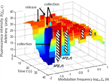
(51) 4.1 Introduction. A schematic diagram, showing the cyclic movement of spherical particles caused by AM DEP towards, and away from a horizontal planar electrode array, is displayed in figure 4.1(a). Each cycle consists of a particle collection phase followed by a release phase. The distribution of particles over space and time is described by the object concentration, c(y, t) and the total number of objects, N, within the system remains constant throughout the experiment, i.e. no particles enter or escape. The corresponding time-dependent particle concentration near the electrode array at =. is shown in figure 4.1(b).. Before switching on the DEP force at the start of the collection phase of the cycle t < tl, figure 4.1(a)(i), the particles are uniformly distributed with initial concentration, cli (the subscripts ‘l’ and ‘i’ denote ‘collection’ phase of cycle and ‘initial’ state). When applying the potential to the electrodes, the action of the pDEP force causes downward particle movement, particularly near the electrode array where the DEP force is strong, figure 4.1(a)(ii). As the concentration further increases near the array, DEP accumulation near the lower boundary results in a depletion layer that steadily rises towards the cap at. = . The cap is located at height ℎ =. −. above the array, as shown.. Eventually the DEP particle flux becomes balanced by thermally driven diffusion, figure 4.1(a)(iii), and approaches the steady state,. =. with concentration,. .. Switching off the ac potential initiates the release phase since there is no longer any pDEP force to trap the particles, and they diffuse into the bulk medium, figure 4.1(a)(iv) eventually reaching initial state at =. . 45 | P a g e.

(52) Figure 4.1. Particle cyclic collection under the action of pDEP force and release after the DEP force is switched off (a) cartoon showing particle distribution (side view) (b) concentration at the array as a function of time showing particle collection (onto the array) and release.. On–off switching can be repeated, as reported for pDEP of DNA [136]. In the scheme where on–off switch periods are sufficiently long for the system to reach steady and initial state in each of the phases, the difference between the steady state and initial concentration is. =. −. . The alternative case when the on–off. switch periods are much shorter than the time required to reach steady and initial states is considered in the following sections.. 46 | P a g e.

(53) 4.2 System model. A schematic of the AM RF DEP system is shown in figure 4.2 The signal generator supplying voltage to the DEP electrode system is assumed to be adjusted so that 100% modulation occurs. The electrical potential at the output is given by, Φ( ) =. where the. [1 +. ( )] × cos(. and. ),. (4.1). are the co-sinusoidal amplitude and angular frequency,. respectively. To distinguish with modulation parameters, the subscript ‘c’ denotes carrier that is analogous to message signalling in electronic communication systems [137]. The modulation signal is a square-wave zero-mean cyclic process with period T , frequency fm = 1/T with subscript ‘m’ denoting modulation, and duty ratio, η, that distinguishes separate positive and negative phases. The modulating signal of the. th. cycle is written as ( )=. ( )=. +1, −1,. +. < < + , < < ( + 1). (4.2). The small time average spatial-temporal force distribution has been further developed using Laplace’s equation to evaluate spatial variation of electric field (peak value) and unit step function [138].. 47 | P a g e.

(54) Figure 4.2. Schematic of ‘on–off’ amplitude modulation (AM) model. The left box shows an AM generator that produces a co-sinusoidal signal with a square-wave envelope. The AM signal is fed to the DEP planar array. The action of DEP process effectively removes the RF carrier, as shown in the right box, thus filtering the signal to a baseband square wave. The output shows diffusion-limited particle transport, quantified near the array, and is represented as a series of ultra-low pass filters (LPFs).. ⟨. {. (. )}∇| ( )|. ( ),. (4.3). normalised electric field, given by. ( )/Φ( ). and. ( ) is a switch function. ( , )⟩ = 2. where the bracket term for DEP force resemble time averaged force, K(x) is the. that is unity (‘on’) at a specified time interval and zero (‘off’) elsewhere. After including the effect of thermally driven Brownian motion, the space-time evolution of concentration, assuming non-interacting particles, is written in differential form as the modified diffusion equation: ( , ). 1 =− ∇∙. ( , ). ( ). ( ) +. ∇ ∙ ∇ ( , ).. (4.4). 48 | P a g e.

(55) 4.3 Concepts and Parameters. Particle motion to the electrode edges depends on the strength of the pDEP. After a certain time tss, the number of particles at the edges will be saturated. This number is dependent on the attracting force. When AM DEP is applied, however, the final number of particles, collected on the electrode edges nmax also depends on the collection-release state (transient or cyclic steady behaviour, figure 4.3) and the frequency of modulation signal. The electrode edges, previously referred to, in reality are small areas of interest around the electrodes. And the motion, away from that area caused by Brownian motion is not instantaneous. Hence the minimum number of particles nmin in AM DEP is also dependent on the collection-release state and the frequency of modulation signal as well as the stochastic force. The cyclic DEP collection and release of particles within a designated volume leads to an important parameter: the difference between the maximum and minimum value of the particle number, for the jth cycle.. This particle number fluctuation, or. amplitude, is defined, Δ. =. −. ,. (4.5). where subscripted terms ‘max’ and ‘min’ denote maximum and minimum particle number. As illustrated in figure 4.3, an important distinction is made between transition and periodic or cyclic steady behaviour. . In the case of the transition. state, the number of particles n at the beginning of jth cycle is less than at the beginning of j+1, [ ] < [( + 1) ]. For alternative to ‘. this number remains constant. An. ’ is a term ‘cyclostationary’, used in information theory, where 49 | P a g e.

(56) system statistics remain unchanged at periodic time points [139, 140]. This periodic equilibrium state implies that the initial condition (IC) and, as a result for constant pDEP force, the amplitude remains constant. The transition from a well-defined DEP amplitude response at ultra-low fm compared with the response being negligible at higher modulation frequencies naturally suggests a DEP ‘modulation bandwidth’. It can be defined as the range of modulation frequencies, fm, such that at Δ (. )≤ Δ (. ),. where ε is an arbitrary cut-off typically,. , (4.6). ≈ 0.1, and subscripts ‘mB’ and ‘mUL’. denote modulation bandwidth and ultra-low modulation that approaches dc (when fm→ 0). The transition state may be of interest when analysing the initial collection rate as in [141], however, this work mainly focuses on the amplitude during the cyclic steady behaviour. This amplitude depends on the magnitude of DEP force, modulation frequency and duty cycle η. Clearly for extreme cases when η = 0 and η = 1, Δ. = 0.. 50 | P a g e.

(57) Figure 4.3 A schematic diagram of a normalised particle number versus time for η=0.6(60% duty cycle). So far the amplitude was presented as the difference in the particle number. And although image analysis tools like ImageJ offer flexible automated system for particle identification and estimation, using particle number for quantitative experimental analysis remains impractical. The fluorescence intensity produced by these particles is used and a normalised amplitude AN is derived instead (section 4.4).. 51 | P a g e.

(58) 4.4 Normalised Amplitude AN. As previously discussed in section 4.3, it is useful to describe the difference in ‘on’ and ‘off’ state in terms of the fluorescence intensity. The normalised amplitude AN was derived for this purpose. The amplitude “A” of the intensity variation for a number of cycles Nc over a video sequence can be defined as the difference between the maximum and minimum intensities over a certain jth cycle:. =. 1. [. ( )−. ( )],. (4.7). represents the spatially averaged fluorescence intensity. For a number of fluorescent particles, ignoring the background effect, it can be written as. ∝. ∆ ∆. ,. is the incident light,. (4.8) is the number of particles, that at the cyclic steady state. consists of a nearly constant minimum and maximum number; and. is the optical. fluorescence constant that is dependent on the size and optical properties of the spheres. ∆ ∆ mean that. is spatially averaged in x and z direction.. Equation 4.7 provides an estimate for the intensity amplitude A as shown in figure 4.4(b). But it is unsatisfactory to use this equation to compare between different experiments, because even though the nominal concentration remains the same, the number of particles close to the electrode array may vary. Also different particle sizes affect A due to the differences in. . Consequently, to compare different 52 | P a g e.

(59) experiments, a normalised value which takes into account an average intensity of the sequence of frames was derived by Bakewell et al. [138] and the resulting value of the normalised amplitude which considers the effect of duty cycle is give in equation 4.9.. =. ∑. 1. ∑. ( )−. (). (). (4.9). The resulting equation enables the comparison between experiments for particles with different diameters. In the equation. is the total number of frames. Provided. that the variations in the aliquot concentration are not too large, the normalised amplitude is a good estimate of the cyclic temporal variation in particle numbers at cyclic steady behaviour.. 4.5 Experimental materials and methods. The fluorescently labelled 0.5 and 1 µm diameter carboxylate modified polystyrene fluorescent spheres FluoSpheres® (F8813 and F8823, Invitrogen, UK) with yellow– green emission λ = 515 nm were diluted 2/1000, 4/1000 and 8/1000 stock. Reverse osmosis water (Millipore, UK) was used to dilute the latex spheres and the final conductivity was measured to be ~1 mS/m (Hanna, HI 8733, UK). 4 µl samples were micro-pipetted (Gilson, UK) on planar castellated microelectrode structure and covered with a coverslip. The electrode arrays were planar, platinum on glass, and made using standard microlithographic methods. The electrodes were mounted on Veroboard (RS components, UK). The height of the flow cell was approximately 160 53 | P a g e.

No results found