FIBER QUADRISECANTS IN KNOT ISOTOPIES

(1)

c

⃝World Scientific Publishing Company

T. FIEDLER

Laboratoire Emile Picard, Universit´e Paul Sabatier, 118 Route Narbonne, 31062 Toulouse, France

fiedler@picard.ups-tlse.fr

V. KURLIN

Department of Methematical Sciences, Durham University, Durham DH1 3LE, UK

vitaliy.kurlin@durham.ac.uk

Accepted 28 June 2007

ABSTRACT

Fix a straight lineLin Euclidean 3-space and consider the fibration of the complement

ofLby half-planes. A generic knotKin the complement ofLhas neither fiber

quadrise-cants nor fiber extreme sequadrise-cants such thatKtouches the corresponding half-plane at 2

points. Both types of secants occur in generic isotopies of knots. We give lower bounds for the number of these fiber secants in all isotopies connecting given isotopic knots. The bounds are expressed in terms of invariants calculable in linear time with respect to the number of crossings.

Keywords: Knot; braid; isotopy; fiber quadrisecant; fiber extreme secant; writhe; trace graph; 1-parameter approach; higher order Reidemeister theorem.

Mathematics Subject Classification 2000: 57M25

1. Introduction

In this paper, we give another application of the main result of [3], namely, thehigher order Reidemeister theorem for one-parameter families of knots. Fix a straight line Lin_R3_{, the}_axis_{. For simplicity assume that}_L_{is horizontal. Consider the fibration}

ϕ : R3₋_L _→ _S1

ϕ by half-planes attached to the axis L. The fibration ϕ can be visualized as an open book whose half-planes are fibers of ϕ. We will study some

distances between isotopic knots in the complement_R3₋_L_.

A knot is the image of aC∞_{-smooth embedding}_S1

→R3

−L. An isotopy of knots is a smooth family_{Kt},t∈[0,1], of smooth knots. The theory of knots in

R3₋_L_{covers the classical knot theory in} _R3 _{and closed braids. An}_n_-braid_β _{is a}

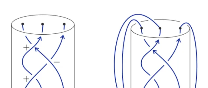
family of ndisjoint strands in a vertical cylinder such that the strands have fixed endpoints on the horizontal bases of the cylinder and they are monotonic in the vertical direction. After identifying the bases of the cylinder in Fig. 1, any braid

1415

J. Knot Theory Ramifications 2008.17:1415-1428. Downloaded from www.worldscientific.com

(2)

[image:2.595.45.389.64.210.2]

Fig. 1. Examples of a braid, a closed braid, a plat knot.

β becomes aclosed braid ˆβ, a link in a solid torus going around the axisL. The boundary circle of the lower base of the cylinder plays the role ofL_{∪ ∞}.

Asecant, atrisecantand aquadrisecant ofK⊂R3₋_L_{is a straight line meeting}

Ktransversally in 2, 3 and 4 points, respectively. A secant meetingKin pointsp, q isextreme if the secant and the tangents ofKatp, qlie in the same plane. Namely, Khas tangencies oforder 1 atp, qwith a plane passing through the secant, i.e. the plane andK are given by {z= 0} and{y = 0, z =x2_} _{in local coordinates near}

p, q. A generic knot has finitely many extreme secants and quadrisecants. If we are interested only in fiber secants respectingϕ, then these geometric features define

codimension 1 singularities in the space of all smooth knotsK_⊂R3

−L.

Definition 1.1. A fiber secant, a fiber trisecant, a fiber quadrisecant of a knot K⊂R3₋_L_{is a straight line meeting}_K_{transversally in 2, 3, 4 points, respectively,}

that lie in a fiber of the fibration ϕ:_R3

−L_→ S1

ϕ. A fiber secant meeting K in pointsp, qis calledextreme ifK has tangencies of order 1 atp, qwith the fiber.

We use fiber secants to measure a distance between diﬀerent embeddings of a knot. A similar distance with respect to Reidemeister moves of type III was studied in [1], see Fig. 4. Reidemeister moves can be performed on a knot K in a small neighborhood of a disk. Reidemeister moves III correspond to triple points in the horizontal disk of a projection, i.e. to vertical trisecants meetingK in 3 points.

The authors of [1] found the minimal number of vertical trisecants in isotopies between diﬀerent representations of a knot. We consider more general features of a knot, namely, quadrisecants in the half-planes of the fibrationϕand estimate their

minimal number in knot isotopies. Arbitrary quadrisecants provide lower bounds for the ropelength of knots [2]. To define our lower bounds, we associate to each knotK_⊂_R3

−Lan oriented graph TG(K), thetrace graph in a thickened torus. Choose cylindrical coordinates ρ,ϕ,λin R3_{, where} _λ_{is the coordinate on the}

oriented axis L, ρ and ϕ are polar coordinates on a plane orthogonal to L. For

(3)

an ordered pair of points (p, q)⊂{ϕ= const}, let τ(p, q) be the angle betweenL and the oriented lineS(p, q) passing first throughpand after throughq. Denote by

ρ(p, q) the distance between S(p, q) and the origin 0 ∈ L. Introduce the oriented thickened torus_T=S1

τ×S1ϕ×R+ρ parametrized byτ,ϕ∈[0,2π) andρ∈R+. Definition 1.2. Take a knotK_⊂_R3

−Lin general position such thatKintersects each fiber ofϕin finitely many points. Map an ordered pair (p, q)⊂K∩{ϕ= const} to (τ(p, q),ϕ,ρ(p, q))_∈ _T. So, each oriented fiber secant ofK maps to a point in the thickened torus_T. The image of this map is thetrace graph TG(K)⊂T.

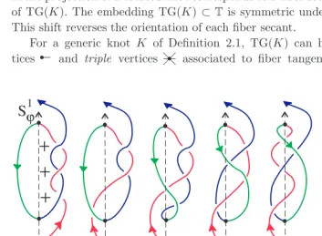
Figure 2 shows the trace graph TG(K) of a long trefoilK going once around a distant horizontal circle L_{∪ ∞}. The fibers there are horizontal planes. The trace graph TG(K) can be visualized as a trace of fiber secants evolving along K. The knots in Fig. 2 are obtained fromKby the rotation around a vertical line. A crossing in the projection of a rotated knot corresponds to a fiber secant ofK, i.e. to a point of TG(K). The embedding TG(K)_⊂T is symmetric under the shiftτ _)→ τ+π.

This shift reverses the orientation of each fiber secant.

For a generic knot K of Definition 2.1, TG(K) can have only hanging ver-tices ! and triple vertices !❅! associated to fiber tangents and fiber trisecants

S

_ϕ

1

S

_ϕ

1

_S

_ϕ

1

S

1

_τ

τ

= 0

τ

=

π

/6

τ

=

π

/3

τ

=

π

/2

τ

=

2 π

/3

τ

=

5 π

/6

τ

=

π

τ

=

π

τ

=

2 π

+

[0]

[1]

[0]

[image:3.595.49.403.331.590.2]

[0]

Fig. 2. The trace graph TG(K) of a long trefoilK.

(4)

S_ϕ1

S1_τ [3]

[3] [3] [3] [3]

[3] [2]

[2] [2] [2] [2]

[2]

[1]

[1] [1] [1] [1]

[1]

σ

[image:4.595.58.394.65.137.2]

3 2 1

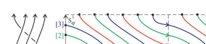
Fig. 3. The trace graph ofσ!3σ2σ1splits into 3 trace circles.

of K, respectively. A double crossing of TG(K) under prτ ϕ : TG(K)→ Sτ1×Sϕ1 corresponds to a pair of parallel secants meeting K in points that lie in a fiber {ϕ= const_}.

Letmbe the linking number of a knotKwith the axisL. It turns out that the trace graph TG(K) splits into a union of orientedtraces (arcs or circles) marked by canonically defined homological markings inZ|m|, whereZ0=ZandZ1={0},

see Definition 2.2. For example, the closure ofσ3σ2σ1∈B4has the trace graph in

Fig. 3, which is a disjoint union of 3 trace circles marked by [1],[2],[3]∈Z4.

Introduce the sign of a crossing in the projection prτ ϕ(TG(K)) as usual, see Fig. 1. We shall define 3 functions on TG(K), which will be invariant under regular isotopy of TG(K), not allowing Reidemeiser moves of type I, see Lemma 3.1.

Definition 1.3. Take a knotK ⊂R3₋_L_{such that lk(}_{K, L}_{) =}_m_̸₌_±_{1 and the}

projection prτ ϕ(TG(K)) has finitely many crossings. For distinct [a],[b] ∈Z|m|−

{0}, theunordered writheWu

a,b(K) is the sum of signs over all crossings of the trace marked by [a] with the trace [b]. The ordered writheWo

a,b(K) is the sum of signs over all crossings, where the trace [a] crosses over the trace [b]. The coordinated writheWc

a,a(K) is the sum of signs over all self-crossings of the trace [a].

We do not consider knotsK⊂R3₋_L_{with lk(}_{K, L}_{) =}_±_{1, because in this case}

TG(K) splits into trace arcs marked by [0] and [1] only, see Definition 2.2. The trace graph TG(K) can be constructed from a plane projection of K, see Lemma 2.4. The writhes of Definition 1.3 depend on a geometric embeddingK_⊂R3

−L, but can be computed in linear time with respect to the number of crossings ofK and change under knot isotopies in a controllable way, see Lemma 3.2.

Theorem 1.4. For isotopic generic knotsK0, K1⊂R3−L, denote byfqs(K0, K1)

andfes(K0, K1) the least number of fiber quadrisecants and fiber extreme secants,

respectively, occurring during all isotopies_{Kt_},t_∈[0,1].

For isotopic knots K0, K1, we have fqs(K0, K1) ≥ ₁₂1 !₀_̸₌_a̸₌_b̸₌₀|Wa,bu (K0)−

Wu

a,b(K1)| and fqs(K0, K1) + 1₆fes(K0, K1) ≥ ₁₂1 !a̸=0|Wa,ac (K0)− Wa,ac (K1)|.

Given isotopic closed braids βˆ0,βˆ1, we get fqs( ˆβ0,βˆ1)≥ ₁₂1 !0̸=a̸=b=0̸ |Wa,bo ( ˆβ0)−

Wo a,b( ˆβ1)|.

(5)

The third lower bound is not less than the first one, but works for closed braids only. The second bound gives another estimate for the number of fiber quadrisecants for closed braids since fiber extreme secants do not occur in braid isotopies. In Example 3.3, we show that the second lower bound can be arbitrarily large.

The lower bounds for the least number of Reidemeiter moves III are computed with exponential complexity in [1], while the writhes of Definition 1.3 can be com-puted in linear time with respect to the number of crossings, see Lemma 2.4. Other applications of the 1-parameter approach to knot theory [3] are in [4, 5].

2. The Trace Graph of a Knot We shall define generic knotsK_⊂_R3

−Land geometric features of knots, considered as codimension 1 singularities in the space of all knots inR3

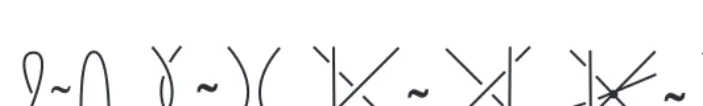
−L. Each singularity is illustrated by a small portion of the projection ofKalong the corresponding secant. For example, a tangent of K maps to a cusp ☎✞in the plane projection along the tangent, while a quadrisecant projects to a quadruple point ✦❛☞☞▲▲ .

Definition 2.1. A knotK_⊂_R3

−L isgenericifK hasnofollowing features: ☞☞

✦_▲▲

❛_{: a fiber quadrisecant intersecting} _K _{transversally in 4 points;}

✟☎_✆✞_✝_{: a fiber trisecant meeting} _K_{in 3 points such that the trisecant lies in the plane} spanned by the tangents ofK at 2 of these points;

✟☎✞: a fiber secant meetingK in 2 points and having a tangency of order 1 withK at one of these points;

✆

✞_{: a fiber secant meeting} _K _{in points}_{p, q} _{such that} _K _{has a tangency of} _order ₂ atpwith the plane spanned by the secant and the tangent ofKatq, i.e. the plane andK are given by{z= 0} and{y= 0, z=x3_}_{in local coordinates near}_p_;

: a fiber tangent having a tangency oforder 2 with Katp, i.e. the tangent and K are given by{y=z= 0}and {y= 0, x2₌_z5_}_{in local coordinates near}_p_;

✞☎, : a fiber trisecant meeting K in 3 points such that K has a tangency of order 1 with the fiber at one of these points;

✆

☎: a fiber tangent meetingK in a point, whereK has a tangency of order 2 with the fiber, i.e. the fiber andK are given locally by_{z= 0_} and_{y= 0, z=x3

}; ✞☎

✝✆, : a fiber secant meeting K in 2 points, whereK has tangencies of order 1 with the fiber.

The singularities of Definition 2.1 can be visualized by rotating a knot around a vertical line. The last singularity represents two local extrema with the same vertical coordinate: they collide under the projection after a suitable rotation.

A trace in the trace graph TG(K) of a knot K is either a subarc ending at hanging vertices or a subcircle of TG(K). A trace passes through triple vertices without changing its direction. The trace graph in Fig. 2 consists of 2 trace arcs.

By Definition 1.2, any point in TG(K) corresponds to a fiber secant ofK and also to an intersection in the projection ofKalong the secant. Hanging vertices and

(6)

[image:6.595.53.405.65.118.2]

I II III IV V

Fig. 4. Reidemeister moves for trace graphs.

triple vertices of TG(K) correspond to cusps ☎✞and triple intersections!❅, respec-tively. Mark also tangent vertices ✞_✝& of degree 2 in TG(K) whose corresponding secants project to tangent points of order 1, see 2 tangent vertices in Fig. 6(iv).

All points of TG(K) apart from the vertices of TG(K) correspond to double crossings with well-defined signs. Associate to such a general point, thesign of the corresponding crossing in the projection. Two close points of TG(K) on diﬀerent sides of a tangent vertex correspond to a couple of crossings with opposite signs like in Reidemeister move II, see Fig. 4. While we travel along a trace of TG(K), the sign does not change at triple vertices, but is reversed at tangent vertices.

To be completely honest we should also considercritical vertices ❜ of degree 2 in TG(K) corresponding to a critical crossing ✞☎in a projection ofK. ThenKhas a fiber secant and another fiber tangent in the same fiber. These critical vertices are local extrema of pr_ϕ : TG(K)→Sϕ1 and denoted by small empty circles in Fig. 6. The critical vertices of TG(K) will not play any role further.

Let us look at the function τ on fiber secants passing through 2 pointsp, q on K. Namely,τ(p, q) is the angle between L and the fiber secant throughp, q. The functionτ(p, q) has a local extremum if and only if the corresponding secant ofK projects to a tangent point, i.e.τchanges its monotonic type at tangent vertices of

TG(K). So, passing through a tangent point of TG(K) reverses the sign of crossing in the projection ofK and simultaneously the monotonic type ofτ.

Definition 2.2. Take a generic knotK_⊂_R3

−Lwith lk(K, L) =m. Split TG(K) by tangent vertices into arcs with associated signs coming from plane projections. Orient each arc so that if the angleτ increases (respectively, decreases) along the

arc then the associated sign of the arc is +1 (respectively,₋1), see Fig. 2.

Any point of TG(K) apart from the vertices of TG(K) is associated to a crossing (p, q) in the projection ofKalong the secant throughp, q∈K. Smoothing crossing (p, q) produces a diagram of a 2-component link. The linking number of the circle L∪ ∞ with the component in which the undercrossing goes to the overcrossing in the original projection ofK is called the homological marking [a]_∈ _Z_|m| of (p, q)

and of the point of TG(K), see Fig. 3.

The trace graph in Fig. 2 splits into 2 trace arcs marked by [0] and [1]. Under the shift τ _)→ τ+π, the homological marking [a] becomes [_|m_|₋a] _∈ _Z_|m|, see

Fig. 3. Recall that a hanging vertex of TG(K) corresponds to a fiber tangent ofK, i.e. to an ordinary cusp in the plane projection along this tangent.

(7)

Lemma 2.3. The trace graph TG(K)of a generic knot K splits into traces with well-defined homological markings. The orientation of edges, introduced in Defini-tion 2.2, provides orientations of all traces of TG(K).

Proof. Consider the sign of a crossing, monotonic type of the functionτand

homo-logical marking as functions of a point in the trace graph TG(K). All these functions remain constant while the projection ofKalong the corresponding secant keeps its combinatorial type. By the classical Reidemeister theorem, a knot projection can change under Reidemeister moves of types I–III, see Fig. 4.

Under Reidemeister move I, a fiber secant ofK appears or disappears, i.e. the corresponding point in the trace graph comes to a hanging vertex. Under Reide-meister move II, two crossings with opposite signs and the same marking appear or disappear. At this moment the function τ reverses its monotonic type. So the

ori-entations of adjacent arcs of TG(K) agree at tangent vertices. Under Reidemeister move III, nothing changes, i.e. all arcs of a trace have the same marking.

The right picture in Fig. 1 shows a plat diagram of a knot Kβ associated to a braidβ. Any knot can be isotoped to a curve having a plat diagram.

Lemma 2.4. LetKβbe a knot with a plat diagram associated to a(2n+1)-braidβ

of braid length l. The trace graph TG(Kβ)can be constructed combinatorially from the diagram ofKβ. The writhes of Definition 1.3can be computed with complexity Cln2_,_{where the constant} _C _{does not depend on}_l _and_n.

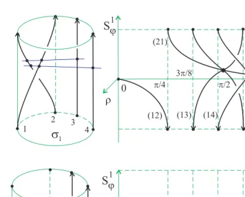
Proof. We describe the trace graphs of elementary braids containing one crossing only. Figure 5 shows the explicit example of the crossingσ1of first two strands in the

4-braid. Firstly, we draw all strands in a vertical cylinder. Secondly, we approximate with the first derivative the strands forming a crossing by smooth arcs.

The monotonic strands in the left pictures of Fig. 5 are denoted by 1,2,3,4. The trace graphs in the right pictures have arcs labeled by ordered pairs (ij), i, j ∈ {1,2,3,4}. The arc (ij) represents crossings, where the ith strand crosses over the jth one. For instance, at the momentτ = 0 the braid σ1 has exactly one

crossing (12), which becomes crossing (21) after rotating the braid throughτ=π/4. Two triple vertices on the upper right picture correspond to two fiber (horizontal) trisecants in the upper left picture. Similarly, we construct the trace graph of a local extremum. The only hanging vertex corresponds to a horizontal tangent.

In general, we split Kβ by fibers of ϕ: _R3

−L_→S1

ϕ into several sectors each of that contains exactly one crossing or one extremum. To each sector we associate the corresponding elementary block and glue them together. The resulting trace graph contains 2l(2n₋1) triple vertices and 2nhanging vertices. Any two arcs in an elementary block have at most one crossing, not more thann2_{crossings in total.}

So each writhe of Definition 1.3 can be computed with complexityCln2_.

(8)

[image:8.595.49.406.65.351.2]

Fig. 5. Half trace graphs ofσ1∈B4 and a local maximum.

Definition 2.5. Denote byΩthe discriminant of knotsKfailing to be generic due to one of the singularities of Definition 2.1. An isotopy of knots _{Kt}, t ∈ [0,1], is generic if the path _{Kt_} intersects Ω transversally. A regular isotopy of trace graphs is generated by isotopy inS1

τ×Sϕ1 and Reidemeister moves II–V.

Any orientations and symmetric images of the moves in Fig. 4 are allowed. Proposition 2.6 is a particular case of the more general higher order Reidemeister theorem [3, Sec. 1.3]. A knot can be reconstructed from its trace graph equipped with labels, ordered pairs of integers, see details in [3, Sec. 6.1].

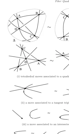
Proposition 2.6. If knots K0, K1⊂R3−L are isotopic, then TG(K0),TG(K1)

are related by regular isotopy and a finite sequence of the moves in Fig.6.

Proof. The singularities of Definition 2.4 are all essential codimension 1 singulari-ties associated to fiber secants and fiber tangents of knots, see [3, Sec. 3]. There are also codimension 1 singularities formed by pairs of fiber secants and fiber tangents

(9)

(i) tetrahedral moves associated to a quadruple point

(ii) a move associated to a tangent triple point

(iii) a move associated to an intersected cusp

(iv) a move associated to a (v) a move associated to

tangency of order 2 a ramphoid cusp

[image:9.595.88.365.53.592.2]

(vi) a move associated to a horizontal triple intersection

Fig. 6. Moves on trace graphs.

(10)

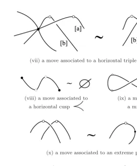
(vii) a move associated to a horizontal triple intersection

(viii) a move associated to (ix) a move associated to

a horizontal cusp a mixed pair

(x) a move associated to an extreme pair

[image:10.595.87.366.64.402.2]

(xi) trihedral move associated to a tangency with

Fig. 6. (Continued)

in the same fiber, but they give rise to trivial moves on trace graphs. For example, the singularity ✞☎, where a fiber secant and a fiber tangent are in the same fiber, leads to the move throwing an arc over a critical vertex.

Any isotopy of knots can be approximated by a generic isotopy of Definition 2.5. Each move of Fig. 6 corresponds to one of the singularities. For instance, when a path in the space of knots passes through a knot with a fiber quadrisecant, the tetrahedral move 6i changes the trace graph by collapsing and blowing up the 1-skeleton of a tetrahedron. A formal correspondence between the singularities and moves was shown in [3, Lemma 5.5].

The moves of Fig. 6 keep the orientation and homological markings of traces. If three traces marked by [a],[b],[c] meet in a triple vertex thenb=a+c(mod_|m_|), where [b] is the marking of the middle trace, see [5, Lemma 3.3]. The trace graph always remains symmetric underτ )→τ+π. Hence, each move of Fig. 6 describes

how to replace a small disk∆ and the symmetric image of∆ underτ _)→τ+πby

another small disk∆′ _{and the symmetric image of}_∆′_{, respectively.}

(11)

3. Proofs of Main Results

Lemma 3.1. The writhes of Definition 1.3are invariant under regular isotopy of trace graphs in the sense of Definition2.5.

Proof. The Reidemeister moves of types II–IV in Fig. 4 do not change the sum of signs in the writhes. The Reidemeister move of type V either adds or deletes a crossing of TG(K), but a trace arc coming to a hanging vertex always has homology marking [0] modulo|lk(K, L)|and is excluded in Definition 1.3.

Lemma 3.2. The moves in Fig.6 keep the writhes of Definition1.3 except

• the move 6(i) changesWu

a,b (a̸=b)by ±2 for at most6 unordered pairs{a, b}; • the move 6(i) changesWo

a,b (a̸=b)by ±1 for at most12ordered pairs (a, b); • the move 6(i) changesWc

a,a either (1)by ±6 for at most2 values ofa, or (2) by _±4 for at most2 values ofaand by _±2for at most2 values ofa, or (3) by ±2 for at most6 values ofa;

• the moves 6(vi), 6(vii) change Wo

a,b (a ̸=b) by ±1 for at most 4 ordered pairs (a, b);

• the moves 6(ix) and6(x)change Wc

a,aby ±1for at most two values ofa. Proof. No crossings appear or disappear in the moves 6(ii)–6(v), 6(viii) and 6(xi). The move 6(i) reverses exactly 3 couples of symmetric crossings. For instance, the arcDB crosses overAC in the left picture of Fig. 6(i), butDB crosses underAC in the right picture. Hence, for at most 6 unordered pairs _{a, b_} with a_̸= b, the unordered writheWu

a,bchanges by±2. Similarly, for at most 12 ordered pairs (a, b), the ordered writheWo

a,bchanges by±1 since exactly one crossing of a trace [a] over a trace [b] either appears or disappears under the move 6(i).

If all the 3 crossings in the disk ∆ in Fig. 6(i) are formed by traces with the same homological marking [a], then the coordinated writhesWc

a,aandW_|cm|−a,|m|−a change by _±6 as required in (1). If two of the above crossings are formed by a trace [a] and the remaining one by a diﬀerent trace [b], then we arrive at (2). The case (3) arises when each of the 3 crossings in ∆ is formed by a diﬀerent trace.

In the moves 6(vi) and 6(vii), the overcrossing arc becomes undercrossing and vice versa, but the sign of the crossing is invariant, i.e.Wu

a,bdoes not change. Each of the moves 6(vi) and 6(vii) deletes exactly one crossing, where a trace [a] crosses over a trace [b], and adds another crossing, where the trace [a] crosses under the trace [b]. Under the symmetryτ_)→τ+π, we get similar conclusions for the traces

marked by [_|m_|₋a] and [_|m_|₋b]. So the ordered writheWo

a,b changes by ±1 for the 4 ordered pairs (a, b), (b, a) and (|m|−a,|m|−b), (|m|−b,|m|−a).

The move 6(ix) adds or deletes a crossing of a trace circle [a] with itself. Hence, only the writhes Wc

a,a and W_|cm|−a,|m|−a change by ±1. The move 6(x) adds or

(12)

deletes a crossing between arcs that belong to traces with the same homological marking [a]. Indeed, a pair of crossings corresponding to these arcs looks like a horizontal version of Reidemeister move II, see Fig. 4. By Definition 2.2, the markings of these crossings are equal. So the conclusion is the same as for the move 6(ix).

Proof of Theorem 1.4. To prove the first lower bound, it suﬃces to show that the right-hand side increases by 1 only if a generic isotopy_{Kt_} passes through a knot with a fiber quadrisecant. By Lemma 3.2, the unordered writhe changes under the move 6(i) associated to a fiber quadrisecant, see the correspondence between singularities and moves in [3, Lemma 5.5]. Six unordered pairs_{a, b_} provide the maximal increase 1 as required. Lemma 3.2 also proves the third lower bound since only the moves 6(i), 6(ii), 6(iv), 6(xi) are relevant for braids.

For the second lower bound, we are interested in crossings whose arcs have the same marking. By Lemma 3.2, the coordinated writhe changes only under the move 6(i) and two moves 6(ix), 6(x) associated to a fiber extreme secant in knot isotopies. Under the move 6(i), the right-hand side increases at most by 1 while under the moves 6(ix) and 6(x) the maximal increase is 1/6 after multiplying by 1/12.

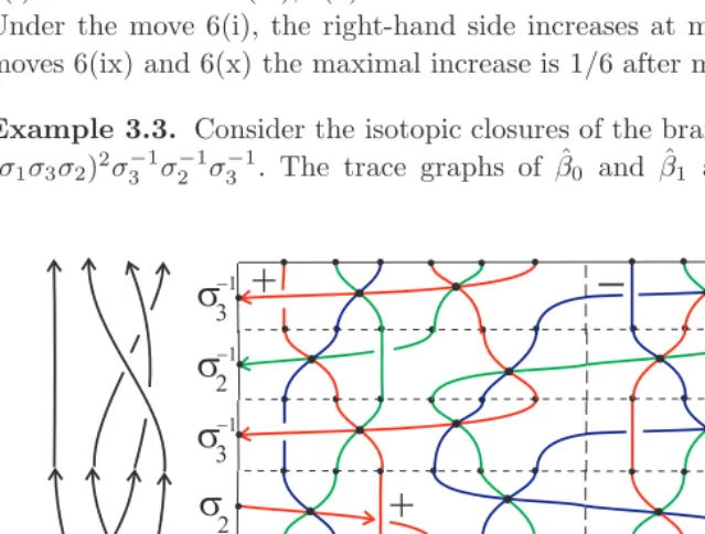
Example 3.3. Consider the isotopic closures of the braidsβ0=σ3σ2σ1 andβ1=

[image:12.595.67.387.354.596.2]

(σ1σ3σ2)2σ3−1σ2−1σ3−1. The trace graphs of ˆβ0 and ˆβ1 are in Fig. 3 and Fig. 7,

Fig. 7. The trace graph of the closure ofβ1= (σ1σ3σ2)2σ−31σ−

1 2 σ−

1 3 .

(13)

respectively. They were constructed by attaching elementary blocks described in the proof of Lemma 2.4. So we assume that the closed braids are given by embeddings into a neighborhood of the torusS1

τ×Sϕ1 located vertically inR3−L.

Both graphs split into 3 closed traces (circles with self-intersections) marked by [1],[2],[3]. The trace graph in Fig. 3 has no crossings, i.e. the writhes of Definition 1.3 vanish. For the trace graph of ˆβ1, the non-zero writhes areW1c,1= 4,W3c,3=−4. The

4 signs + and 4 signs₋are shown in Fig. 7. The second lower bound of Theorem 1.4 implies that any isotopy connecting the closed braids ˆβ0,βˆ1 involves at least one

fiber quadrisecant. The conclusion is the same for the closures ofβ0γ,β1γ, whereγ

is any pure 4-braid, i.e. the permutation generated by γis trivial.

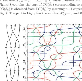
Consider the 4-braidβ = (σ1σ3σ2)2(σ−11σ− 1 3 σ−

1

2 )2 in Fig. 8 and the sequence

of the braids βn = βn−1β1, n ≥ 1, whose closures are isotopic to ˆβ0, see Fig. 3.

Figure 8 contains the part of TG( ˆβn) corresponding to a single factorβ in βn. So TG( ˆβn) is obtained from TG( ˆβ1) by insertingn−1 copies of Fig. 8 at the bottom of

Fig. 7. The part in Fig. 8 has the writhesWc

1,1= 3 andW3c,3=−3. Hence, TG( ˆβn)

β

σ

3 1 −1 −1 −1 −1 −1 −1 3 3 2 2 2 2 3 1 1 1 [1] [1] [1] [1] [1] [1] [2] [2] [2] [2] [3] [3]

+

−

+

[image:13.595.66.388.279.596.2]

[1] [2] [3] [1] [2] [1] [3] [2] [1] [3] [2] [3]

Fig. 8. The part of the trace graph for the factorβ= (σ1σ3σ2)2(σ1−1σ−

1 3 σ−

1 2 )2.

(14)

hasWc

1,1 = 3n+ 1 and W3c,3=−3n−1. By Theorem 1.4, any isotopy connecting

the closures ofβ0 andβn involves at least 3n₁₂+1 fiber quadrisecants. So the second lower bound of Theorem 1.4 can be arbitrarily large.

Acknowledgments

The authors thank Hugh Morton and the anonymous referee for useful comments. The second author was supported by Marie Curie Fellowship 007477.

References

[1] J. S. Carter, M. Elhamdadi, M. Saito and S. Satoh, A lower bound for the number of

Reidemeister moves of type III,Topol. Appl.153(2006) 2788–2794.

[2] E. Denne, Y. Diao and J. M. Sullivan, Quadrisecants give new bounds for ropelength, Geom. Topol.10(2006) 1–26.

[3] T. Fiedler and V. Kurlin, A one-parameter approach to knot theory, preprint, math.GT/0606381.

[4] T. Fiedler, Isotopy invariants for closed braids and almost closed braids via loops in stratified spaces, preprint, math.GT/0606443.

[5] T. Fiedler and V. Kurlin, Recognizing trace graphs of closed braids, preprint, arXiv: 0808.2713.