Gesture Recognition Using Hidden Markov Models Augmented with Active Difference Signatures

Rochester Institute of Technology

RIT Scholar Works

Theses Thesis/Dissertation Collections

12-2014

Gesture Recognition Using Hidden Markov

Models Augmented with Active Difference

Signatures

Himanshu Kumar

Follow this and additional works at:http://scholarworks.rit.edu/theses

This Thesis is brought to you for free and open access by the Thesis/Dissertation Collections at RIT Scholar Works. It has been accepted for inclusion in Theses by an authorized administrator of RIT Scholar Works. For more information, please [email protected].

Recommended Citation

Gesture Recognition Using Hidden Markov Models

Augmented with Active Difference Signatures

by

Himanshu Kumar

A Thesis Submitted in Partial Fulfillment of the Requirements for the Degree of Master of Science in Computer Engineering

Supervised by

Dr. Raymond Ptucha

Department of Computer Engineering Kate Gleason College of Engineering

Rochester Institute of Technology Rochester, NY

Dec 2014

Approved By:

_____________________________________________ ___________ ___

Dr. Raymond Ptucha

Primary Advisor – R.I.T. Dept. of Computer Engineering

_ __ ___________________________________ _________ _____

Dr. Andreas Savakis

Secondary Advisor – R.I.T. Dept. of Computer Engineering

_____________________________________________ ______________

Dr. Nathan D. Cahill

Dedication

I dedicate my thesis work to my family and friends. A special feeling of gratitude to my

loving parents, Ashok and Saroj Choudhary, whose words of encouragement

continuously pushed me towards my goal. I would also like to thank Ms. Kajal

Acknowledgements

First and foremost I offer my sincerest gratitude to my advisor, Dr. Raymond Ptucha,

who has supported me throughout my thesis with his patience and knowledge whilst

allowing me the room to work in my own way. I attribute the level of my Masters degree

to his encouragement and effort and without him this thesis, too, would not have been

completed or written. One simply could not wish for a better or friendlier advisor.

Besides my advisor, I would like to thank the rest of my thesis committee, Dr. Andreas

Savakis and Dr. Nathan Cahill for their encouragement, insightful comments and hard

Abstract

Table of Contents

1. Introduction ...1

2. Background ...3

2.1 Related Work ... 3

2.2 Gesture Recognition ... 10

2.3 Clustering ... 13

2.4 Hidden Markov Model ... 15

2.4.1 Definition of HMMs ... 21

2.4.2 Model of HMMs ... 22

2.4.3 The Three Basic Problems for HMM ... 23

2.5 Active Difference Signature ... 27

3. Methodology ...33

4. Experiments and Results ...47

4.1 Dataset and Experimental Methodologies ... 47

4.2 Experimental Results ... 50

4.3 Future Work ... 60

5. Conclusion ...62

Bibliography ...63

List of Figures

Figure 1: Block Diagram of Gesture Recognition Framework ... 12

Figure 2: Clustering of Data ... 15

Figure 3: Markov Model for Gesture Problem ... 17

Figure 4: Ergodic Model ... 22

Figure 5: Left-Right Model ... 23

Figure 6: Left-Right Banded Model ... 23

Figure 7: Overview of Active Difference Signature Framework ... 28

Figure 8: Difference Signature and Motion Signature Curve ... 29

Figure 9: Active Difference Signature vs. Difference Signature for Joints ... 32

Figure 10: Skeleton Joints ... 33

Figure 11: Skeleton Joints ID for ChaLearn ... 34

Figure 12: Gesture Recognition Framework ... 35

Figure 13: Hand Motion Signal ... 36

Figure 14: Gesture Detection Using Hand Motion ... 37

Figure 15: Joint Angles From Skeleton Data ... 40

Figure 16: Elbow Joint Angle ... 41

Figure 17: Relative Position of Hand With Respect to Head ... 42

Figure 18: Skeleton JointID for MSR3D ... 45

Figure 19: Italian Sign 1-10 ... 48

Figure 20: Italian Sign 11-20 ... 48

Figure 21: Confusion Matrix for MSR3D ... 52

Figure 22: Jaccard Index vs. Hidden States ... 54

Figure 23: Accuracy vs. Hidden States ... 55

Figure 24: Variable State vs. Fixed State for ChaLearn ... 59

Figure 25: Variable State vs. Fixed State for MSR3D ... 60

List of Tables

Table 1: Transition Probability Matrix for Gesture Problem ... 17

Table 2: Probability of Hand velocity for Gesture Problem... 18

Table 3: MSR3D Result ... 51

Table 4: ChaLearn Result ... 53

Table 5: Result on ChaLearn with and w/o Active Difference Signature ... 56

Table 6: Result on MSR3D with and w/o Active Difference signature ... 56

Table 7: Result on ChaLearn with Different Types of HMMs ... 56

Table 8: Result on MSR3D with Different Types of HMMs ... 57

Table 9: Active Body Parts Based Experiment Result for ChaLearn ... 57

Table 10: Active Body Parts Based Experiment Result for MSR3D ... 58

Table 11: Joint Angle Based Experiment Result for ChaLearn ... 58

Glossary

JOI Joint of interest

HMM Hidden Markov Model

LR Left - Right HMM

LRB Left - Right Banded HMM

MSR3D Microsoft Action 3D

DHMM Discrete Hidden Markov Model

VQ Vector Quantization

VC Vector Codebook

MHI Motion History Image

AU Action Units

SIFT Scale-Invariant Feature Transform SVM Support Vector Machine

ASL American Sign Language

HRI Human-Robot Interaction

Chapter 1

Introduction

Human gestures are non-verbal body actions used to express information and can

typically be instantly recognized by humans. Gestures are used in sign language, convey

messages in noisy environments, and to interact with machines [1]. Automatic gesture

recognition from continuous video streams has a variety of potential applications from

smart surveillance to human-machine interaction to biometrics [2, 3].

There are two categories of gesture recognition, isolated recognition and

continuous recognition [5]. Isolated gesture recognition is based on the assumption that

each gesture can be individually extracted in time, from the beginning to end of gesture

[6]. Continuous recognition has the additional challenge of spotting and recognizing a

gesture in continuous stream [6]. In the real world scenarios, gestures are continuous in

nature, without any explicit pause or break between individual gestures. Thus the

recognition of such gestures closely depends on the segmentation; i.e. determining start

and end frame of each gesture in a continuous stream of gestures [4]. Spatiotemporal

variability [7] refers to dynamic variations in movement and duration, even for same

gesture. The intermediate motion between two consecutive gestures is termed as

transitional motion.

Many researchers have used multi-modal gesture information to tackle the

problem of segmentation ambiguity [7], differentiating between meaningful gestures and

transitional motions, and recognition. The use of multi-modal information i.e. depth,

RGB, audio and skeleton joints, introduces high latency in real time applications. The

goal of this thesis is to introduce a system which uses only skeleton joint information to

real-time applications. The proposed method uses skeleton joints along with active difference

signatures [30] for gesture recognition. The method has shown good accuracy on

ChaLearn and MSR3D Action dataset. On the ChaLearn dataset, the proposed method

gives accuracy of 0.58 when Hidden Markov Model is augmented with active difference

signature against 0.51 when no active difference signatures are used. While on MSR3D

dataset, the proposed method got 80.70% accuracy using leave-one-subject out

cross-validation with active difference signature against 69.05% when no active difference

Chapter 2

Background

2.1. Related Work

A vast amount of research has been done on gesture recognition. Most of it has

been based on two-dimensional computer vision methods or some augmented input

devices such as colored or wired "data gloves". The performance of earlier methods such

as identifying gestures using one or more conventional cameras is highly dependent on

lighting conditions and camera angle. With the introduction of the Kinect camera,

virtually all state of art gesture recognition research has shifted to using RGB-D data,

where the D is a depth channel. The Kinect based approach has improved the user

interactivity, user comfort, system robustness, and ease of deployment.

Patsadu et al. [8] demonstrated the high potential of using Kinect for human

gesture recognition. They used twenty joint locations returned by Kinect to classify three

different human gestures of stand, sit down and lie down. They showed that using

different machine learning algorithms such as Support Vector Machines (SVM), decision

trees, and naive Bayes, they could achieve an average accuracy rate of 93.72%. A neural

network trained with backpropagation achieved 100% accuracy.

Starner et al. [9] used a view based approach with single camera to extract 2D

features as the input to a Hidden Markov Model (HMM) for continuous American Sign

Language (ASL) recognition. They achieved an accuracy of 92% with 40 different signs.

They used a single color camera to track hand shape, orientation and trajectory. The

downside is the user was required to wear inexpensive colored gloves to facilitate the

made gloves for tracking finger movement with similar performance. These systems have

mostly concentrated on finger signing, where the user spells each word with individual

hand signs, each corresponding to a letter of the alphabet [11]. These approaches

compromised user comfort and were shown to be accurate only in a controlled

environment.

Huang and Huang [12] used skeletal joints from the Microsoft Kinect sensor

along with SVM classification to achieve a recognition rate of 97% on signed gestures.

The dataset comprised of fifty samples from two users each. They implemented ten ASL

signs, all of which were based on arm movement. Their approach fails in case of gestures

that involve finger and facial movement as skeleton tracking does not provide finger and

facial movement information. Another limitation was that they used a fixed duration of

ten frames, restricting the speed of which a sign can be made.

Biswas and Basu [13] used depth images from the Kinect sensor for hand gesture

recognition. They showed that depth data along with the motion profile of the subject can

be used to recognize hand gestures like clapping and waving. They presented a lesser

compute intensive approach for hand gesture recognition, and shown the accuracy of the

system can be further improved by using skin color information from RGB data. Agarwal

et al. [14] used the depth and motion profile of the image to recognize Chinese number

sign language from the ChaLearn CGD 2011, [15] gesture dataset. They used low level

features such as depth and motion profiles of the each gesture to achieve an accuracy of

92.31%. The authors suggested the accuracy may be further improved if high level

features like optical flow information or motion gradient information were incorporated

Zafrulla et al. [16] investigated the use of Kinect for their currently existing

CopyCat system which is based on the use of a colored glove. They achieved accuracy

rate of 51.5% and 76.12% on ASL sentence verification in seated and standing mode

respectively which is comparable to the 74.82% verification rate when using the current

CopyCat system. They used a larger dataset of 1000 ASL phrases. They used the depth

information for ASL phrase verification, whereas the RGB image stream is used to

provide live feedback to the user. They used the skeleton tracking capability of the Kinect

along with depth information to accurately track the arm and hand shape respectively.

Vogler and Metaxas [17] designed a framework for recognizing isolated as well

as continuous ASL sentences from three dimensional data. They used multiple camera

views to facilitate three dimensional tracking of arm and hand motion. They partly

addressed the issue of co-articulation, whereby the interpretation of the sign is influenced

by the preceding and following signs, by training a context-dependent Hidden Markov

Model. They successfully showed that three dimensional features outperform

two-dimensional features in recognition performance. Furthermore, they demonstrated that

context-dependent modeling coupled with HMM vision models improve the accuracy of

continuous ASL recognition. With the 3D context-dependent model, they achieved

accuracy of 89.91% for continuous ASL signs with a test set of 456 signs.

Nianjun and Lovell [18] presented a paper in which they described a Hidden

Markov Model (HMM) based framework for hand gesture detection and recognition. The

observation sequence for the HMM model is formed by features extracted from the

segmented hand. They performed vector quantization on the extracted features by using

better than classic template based methods. They also compared two training algorithms

for the HMMs; 1) the traditional Baum-Welch and 2) the Viterbi path counting method.

By varying the model structure and number of states, they found that both methods have

reasonable performance.

Yang and Xu [19], proposed a method for developing a gesture based system

using a multi-dimensional HMM. They converted the gestures into sequential symbols

instead of using the geometric features. A multi-dimensional HMMs models each

gesture. Instead of using geometric features they used features like global transformation

and zones. They achieved an accuracy of 99.78% using 9 isolated gestures. Their method

did not work quite well in case of continuous gestures.

Nhan et al. [41] investigated the application of HMM in the field of Human-Robot

Interaction (HRI). This paper introduced a novel approach for HRI in which not only the

human can naturally control the robot by hand gesture, but also the robot can recognize

what kind of task it is executing. A 2-stage Hidden Markov Model is used, whereby the

1st stage HMM recognizes the prime command gestures, and the 2nd stage HMM utilizes

the sequence of prime gestures from the 1st stage to represent the whole action for task

recognition. Another contribution of this paper is the use of output Mixed Gaussian

distribution in HMM to improve the recognition rate.

Wilson et al. [42] presented a method for the representation, recognition, and

interpretation of parameterized gestures. Parameterized gestures are those gestures that

exhibit a systematic spatial variation; one example is a point gesture where the relevant

parameter is a two dimensional direction. In their approach, they extended the standard

variation in the output probabilities of the HMM states. The results demonstrate the

recognition superiority of the parametric HMM (PHMM) over standard HMM

techniques, as well as greater robustness in parameter estimation with respect to noise in

the input features.

Yang et al. [43] proposed an HMM-based method to recognize complex

single-hand gestures. The gestures samples were collected by using common web cameras. They

used the skin color of the hand to segment hand area from the image to form a hand

image sequence. To split continuous gestures they used a state-based spotting algorithm.

Additional features included hand position, velocity, size, and shape. 18 different hand

gestures were used, where each hand gesture was performed 10 times by 10 different

individuals to achieve an accuracy of 96.67%. The disadvantage of this method is that it

used skin color for segmentation which is very sensitive to the lighting conditions.

Yang and Sarkar [44] addressed the problem of computing the likelihood of a

gesture from regular, unaided video sequences, without relying on perfect segmentation

of the scene. They presented a method which is an extension of the HMM formalism,

which they called frag-HMM. This formulation, does not match the frag-HMM to one

observation sequence, but rather to a sequence of observation sets, where each

observation set is a collection of groups of fragmented observations. This method is able

to achieve recognition performance within 2% of that obtained with manually segmented

hands and about 10% better than that obtained with segmentations that use the prior

knowledge of the hand color on the publicly available dataset by Just and Marcel [45].

Eickeler et al. [46] presented the extension of an existing vision based gesture

position independent recognition, rejection of unknown gestures, and continuous online

recognition of spontaneous gestures. To facilitate the rejection of unknown gestures,

gestures of the baseline system were separated into a gesture vocabulary and gestures

used to train the filler models, which are defined to represent all other movements. This

system is able to recognize 24 different gestures with an accuracy of 92.9%.

Gaus et al. [48] found fixed state HMM gave the highest rate of recognition

achieving 83.1% over variable state HMM. The gestures were based on the movement of

each right hand (RH) and left hand (LH), which represented the words intended by

signer. Their HMM based system had features like gesture path, hand distance and hand

orientations which were obtained from RH and LH. While training HMM states, they

introduced fixed states and variable states. In the fixed states method, the number of

states are fixed for all gestures and for variable states, the number of states is determined

by the movement of the gesture.

Shrivastava [49] developed a system using OpenCV which is not only easy to

develop but also its recognition rate is so fast that it can be practically used for real-time

applications. The whole system is divided into the three stages of detection and tracking,

feature extraction, and training and recognition. The first stage uses an unconventional

approach of application of CIE L*a*b* color space for hand detection. The process of

feature extraction requires the detection of the hand in a manner which is invariant to

translation and rotation. For training, the Baum-Welch algorithm with Left-Right Banded

(LRB) topology is applied and recognition is achieved by forward algorithm with an

The method presented by Cholewa and Głomb [50], describes choosing the

number of states of a HMM based on the number of critical points in the motion capture

data. Critical points are determined as the points at the end of the sampling interval, local

maxima and local minima of a data sequence. This work used the publicly available

dataset, IITiS gesture database, which contains a recording of 22 hand gestures.

Compared to the standard approach, this method offers a significant performance gain,

where the score of HMMs using critical points as states is, on average, in the upper 2% of

the results.

Vieriu et al. [52] describes a background invariant Discrete Hidden Markov

Model based recognition system where hand gestures are modeled using Markovian

chains along with observation sequences extracted from the contours of the gestures.

They also demonstrated that Discrete HMM (DHMM) outperforms its counterpart when

working on challenging samples collected from Kinect. They used the same dataset as

[52] and achieved an accuracy of 93.38% on test data.

Several methods have been used for gesture recognition: template matching [20],

dictionary lookup [21], statistical matching [22], linguistic matching [23] and neural

networks [24]. Template matching systems are easy to train because the prototypes in the

system are exemplar frames. However, the use of a large number of templates makes it a

compute intensive method. Dictionary lookup techniques are efficient for recognition

when features are sequences of tokens from a small alphabet. The drawback for this

system is that it is not robust. Statistical matching methods employ statistics of example

feature vectors to derive classifiers. Some statistical matching methods make an

systems tends to be poor when the assumptions are violated. The linguistic approach tries

to apply automata and formal language theory to reformulate as a pattern recognition

problem. The major problem with this approach is the need of supplying a grammar for

each pattern class. Neural networks have been successfully applied to solve many pattern

recognition problems. Their major advantage is that they are built from a large number of

simple elements which learn and are able to collectively solve complicated and

ambiguous problems. Unfortunately the best performance neural networks have many

layers and nodes which require large training requirements.

2.2. Gesture Recognition

Gestures are expressive, important body motions involving physical movements

of the fingers, hands, arms, head, face, or body with the intent of: 1) conveying

meaningful information or 2) interacting with the environment [60]. Gestures can be

static (the user assumes a certain pose or con-figuration) or dynamic (with preparation,

stroke, and retraction phases). Some gestures also have both static and dynamic elements,

as in sign languages.

Static gestures can be described in terms of hand shapes. Posture is the

combination of hand position, orientation and flexion observed at some time instance.

Static gestures are not time varying signals and can be understood from still captures in

time such as a picture of a smile or angry face [62].

Dynamic Gesture is a sequence of postures connected by motions over a short

time span. In video sequences, the individual frames define the posture and the video

sequence define the gesture. Dynamic gestures have recently been used to interact with

The applications of gesture recognition are many, ranging from sign language

through medical rehabilitation to virtual reality. Gesture recognition has wide-ranging

applications [61] such as the following:

 visual communication for the hearing impaired;

 enabling very young children to interact with computers;

 designing techniques for forensic identification;

 recognizing sign language;

 medically monitoring patients’ emotional states or stress levels;

 lie detection;

 navigating and/or manipulating in virtual environments;

 communicating in video conferencing;

 distance learning/tele-teaching assistance;

 monitoring automobile drivers’ alertness/drowsiness levels, etc.

The various techniques used for static (pose) gesture recognition include [63]:

Template Matching

Neural Networks

Pattern Recognition Techniques

While, the techniques used in dynamic gesture recognition include [63]:

Time Compressing Templates

Dynamic Time Warping

Hidden Markov Models

Time-delay Neural Networks

Particle filtering and Condensation algorithm

Finite state machine

The automatic recognition of dynamic or continuous gestures requires temporal

segmentation. Often one needs to specify the onset and offset of a gesture in terms of

frames of movement, both in time and in space. This is the most complex part of the

entire gesture recognition framework. Most of the researchers classify gesture recognition

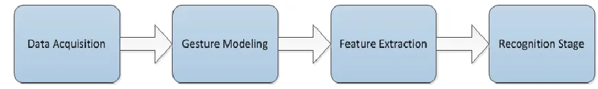
system into four main steps. These steps are: 1) Data acquisition; 2) Extraction method or

gesture modeling; 3) features estimation/extraction, and 4) classification or recognition as

illustrated in Figure 1.

Figure 1: Block diagram of gesture recognition framework.

2.2.1 Data Acquisition

This step is responsible for collecting the input data which are the hand, face or

body imagery. This data is often collected from RGB camera, data gloves or depth

camera like Kinect. If a depth augmented camera is used, data is typically given as RGB

image, depth image and skeleton joint coordinates.

2.2.2 Gesture Modeling

Gesture modeling is concerned with the fitting and fusing the input gesture into

convergence to a unified set of gestures [63]. The pre-processing steps are typically

normalization, removal of noise, gesture segmentation etc. This stage makes the input

data invariant to subject's size, shape and location in the frame. The gesture segmentation

is a complex task and is very critical for the accuracy of the gesture recognition

framework.

2.2.3 Feature Extraction

After gesture modeling, the feature extraction should be robust to large input

variance as the fitting is considered the most difficult task in gesture recognition. Features

can be the location of hand/palm/fingertips, joint angles, or any emotional expression or

body movement. The extracted features might be stored in the system at training stage as

templates or may be fused with some recognition devices such as neural network, HMM,

or decision trees [63].

2.2.4 Recognition Stage

This stage is considered to be a final stage for gesture system and the

command/meaning of the gesture should be clearly identified. This stage usually has a

temporal classifier that can attach each input testing gesture to the closest matching class.

The input to this stage is an unseen test data sequence along with the model parameters

learned from training.

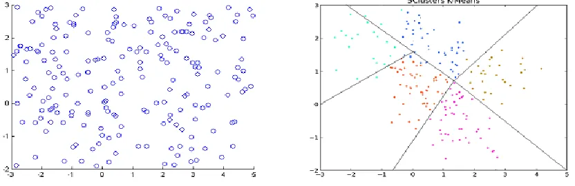
2.3. Clustering

Clustering algorithms partition data objects (patterns, entities, instances,

observances, units) into a certain number of clusters (groups, subsets, or categories) [53].

two points in the cluster is less than the distance between any point in the cluster and any

point not in it”. Clearly, a cluster in these definitions is described in terms of internal

homogeneity and external separation [54,55,56], i.e., data objects in the same cluster

should be similar to each other, while data objects in different clusters should be

dissimilar from one another. Usually similarity is defined as proximity of the points as

measured by a distance function, such as the Euclidean distance of feature vectors in the

feature space. However, measures of other properties, such as vector direction, can also

be used. The method of finding the clusters may have a heuristic basis or may be

dependent on minimization of a mathematical clustering criterion.

In the field of gesture recognition, vector quantization is clustering using the

Euclidean distance measure; however, many new terms are used. The clusters of a

classifier are now called the quantization levels of a vector quantization (VQ) code book.

Furthermore, the distance of each sample to the mean of its enclosing cluster is no longer

a measure of similarity but rather a measure of distortion. The goal of VQ is to find the

set of quantization levels that minimizes the average distortion over all samples.

However, finding the codebook with the minimal average distortion is intractable.

Nevertheless, given the number of clusters, convergence to a local minimum can be

achieved through the simple K-means algorithm [57]:

1. Randomly assign each sample of the data to one of K clusters. The number of

clusters is a predefined parameter which is varied during training.

2. Compute the sample mean of each cluster.

3. Reassign each sample to the cluster with the corresponding nearest mean.

Figure 2: Clustering of data. (left) collection of data. (right) Vector quantization showing the

clusters.

Although it can be proved that the procedure will always terminate, the K-means

algorithm does not necessarily find the most optimal configuration, corresponding to the

global objective function minimum. The algorithm is also significantly sensitive to the

initial randomly selected cluster centers. The K-means algorithm can be run multiple

times to reduce this effect.

In this thesis, the clustering method is as follows. First, all the data are collected

into a single set of observation vectors. Next, vector quantization groups the data points

into clusters.

2.4. Hidden Markov Model

The HMM approach to gesture recognition is motivated by the successful

application of HMM to speech recognition problems. The similarities between speech

and gesture suggest that techniques effective for one problem may be effective for the

other as well. Inherently, HMMs can model temporal events in an elegant fashion. As

gestures are a continuous motion phenomenon on a sequential time series, HMMs are a

Before describing the Hidden Markov Model, it is necessary to describe its

foundation, the Markov Process. A Markov process consists of two parts: 1) a finite

number of states; and 2) transition probabilities for moving between those states. For

example, on a given day a person might be happy, sad or feel a sense of ennui. These

would be the states of the Markov Process. The transition probabilities represent the

likelihood of moving between those states - from a state of happiness on one day to state

of sadness the next.

The Markov process provides a powerful way to simulate real world processes,

provided a small number of assumptions are met. These assumptions, called Markov

Properties, are: a fixed set of states, fixed transition probabilities, and the possibility of

getting from any state to any other state through a series of transitions.

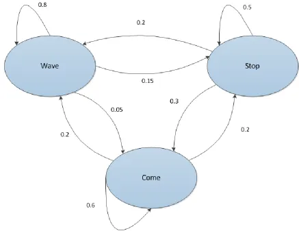
The Markov Model can be better explained by an example. Assume there is a

person who is performing three gestures, one after another. The three gestures are: 1)

Wave; 2) Stop; and 3) Come.

Through this example, Markov analysis can predict the probability of the next

gesture being come, given that previous gesture was wave and current gesture is stop. For

this problem, let's make a first order Markov assumption which states that, the probability

of a certain observation at time n only depends on the observation On-1 at time n-1.

). | ( ) ..., , , |

(O_n O_n1 O_n2 O₁  P O_n O_n1

P ₍₁₎

The joint probability of a certain observation sequence{O1,O2,...,On}, using

Markov assumption is given by (2).



 

 n

i

i i

n P O O

O O O P

1

1 2

1, ,..., ) ( | ).

(

The transition probability matrix for the given problem is shown in Table 1:

Table 1: Transition Probability Matrix.

Current Gesture Next Gesture

Wave Stop Come

Wave 0.8 0.15 0.05

Stop 0.2 0.5 0.3

Come 0.2 0.2 0.6

The Markov Model for the given problem based on the above probabilities is

shown in Figure 3:

Using the Markov assumption and the transition probabilities in Table 1, this

problem translates into:

) |

( ) ,

|

(O₃ come O₂ stop O₁ wave PO₃ come O₂ stop

P      

= 0.3

Thus the probability of next gesture being come is 0.3. This explains the Markov

assumption and Markov Models. So, what is Hidden Markov Model? Well, suppose

instead of direct knowledge of the gesture being performed, i.e. state of the Markov

Process, an observer makes some observations such as joint angle or joint velocity, and

based on a series of past observations, the observer can make a probabilistic guess of the

next gesture. The specific state, i.e. gesture in this case, is hidden from the observer, and

the observer can only make a guess based on past observations. The models which can

simulate these types of processes are called Hidden Markov Models. Once again, an

example is used to clarify the concept of Hidden Markov Model.

Assume the observer is locked inside the room and can't directly observe the

gesture being performed. However, the observer has information about hand velocity.

Let's suppose the probability of observation (hand velocity > threshold or hand

velocity < threshold) is shown in Table 2:

Table 2: Probability of hand velocity greater than threshold.

Gesture Probability of hand velocity greater than threshold (Y)

Stop 0.1

Wave 0.8

The equation for the gesture Markov process before the observer was locked

inside the room was (2). However, in this problem the actual gesture being performed is

hidden from the observer. Finding the probability of a certain gesture

) , ,

(wave stop come

s_i can only be based on the observation O_i with O_i = Y , if the hand

velocity is greater than threshold at observation i, and O_i = N if the hand velocity is

below threshold. This conditional probability P(s_i |O_i) can be written according to

Bayes' rule: ) ( ) ( ) | ( ) | ( i i i i i i O P s P O s P O s

P  (3)

or for n gestures , and gesture sequence S = {S1,..., Sn}, as well as hand velocity

sequence O = {O1,..., On}

) ,..., ( ) ,..., ( ) ,..., | ,..., ( ) ,..., | ,..., ( 1 1 1 1 1 1 n n n n n

n _{P O O}

s s P O O s s P O O s s

P  (4)

Using the probability P(s₁,...,s_n)of a Markov weather sequence from above, and

the probability P(O₁,...,O_n)of seeing a particular sequence of hand velocity events (e.g.

Y, N, Y), the probability P(s₁,...,s_n |O₁,...,O_n)can be estimated as



 n i i i O s P 1 ) |

( , if one

assumes that, for all i, the s_i, O_i are independent of all s_i and O_i , for all ji.

As the probability of the hand velocity being greater than the threshold is

independent of the gesture being performed, one can omit the probability of hand velocity

from (4). To measure the probability, a new term called likelihood, L, is introduced.

Using the first order Markov assumption, likelihood L is given by (5).





n O O P s O P O O

s s L 1 1 1 1

1,..., | ,..., ) ( | ). ( | )

Now, suppose the observer cannot see the "wave" gesture being performed,

however, strategically placed accelerometers on each hand of the actor inform the

observer the hand velocity is greater than threshold, Y. Using this hand velocity

information, the observer has to predict what gesture is being performed. To predict the

gesture being performed, the likelihood of each gesture is calculated given the velocity

information. First calculate the likelihood of the gesture being wave using (5):

) | ( ) | ( ) , | ( 1 2 2 2 2 1 2 wave s wave s P wave s Y O P Y O wave s wave s L        

= 0.8 * 0.8 = 0.64

then the likelihood of gesture being come is:

) | ( ) | ( ) , | ( 1 2 2 2 2 1 2 wave s come s P come s Y O P Y O wave s come s L        

= 0.3 * 0.05 = 0.015

and finally for the likelihood of gesture being stop :

) | ( ). | ( ) , | ( 1 2 2 2 2 1 2 wave s stop s P stop s Y O P Y O wave s stop s L        

= 0.1 * 0.15 = 0.015

The maximum likelihood among the three choices is 0.64 and so most probably

the gesture being performed is wave.

HMM's are statistical methods that model spatiotemporal information in a natural

way. They have elegant and efficient algorithms for learning and recognition, such as

2.4.1 Definition of HMMs

An HMM consists of N states S1, S2, ... , SN, together with transition probabilities

between states. The system is in one of the HMM's states at any given time. At regularly

spaced discrete time intervals, the system evaluates transitioning from its current state to

a new state [6]. Each transition has a pair of probabilities: A) a transition probability

(which provides the probability for taking the transition from one state to another state),

and B) an output probability or emission probability (which defines the conditional

probability of emitting an output symbol from a finite alphabet given a state) [7]. A

formal characterization of HMM is as follows:

 { S1, S2, S3,..., SN } - A set of N states. The state at time t is denoted by the

random variable qt .

 { V1, V2, V3, ..., VM } - A set of M distinct observation symbols, or a discrete

alphabet. The observation at time t is denoted by random variable Ot. The

observation symbol corresponds to the physical output of the system being

modeled.

 A = { aij } - An N x N matrix for the state transition probability distribution

where aij, is the probability of making transition from state si to state sj :

aij = P(qt+1 = sj | qt = si), where q is state at a given time t

 B = { b j (k) } - An N x M matrix for the observation symbol probability

distributions where bj(k) is the probability of emitting Vk at time t in state s j :

bj (k) = P( O t = V k | q t = s j) .

 П = { Пi } - The initial state distribution where Пi is the probability that

Пi = P ( q1 = s i) .

Since A, B and П are probabilistic, they must satisfy the following constraints:









j k





Following the convention, a compact notation λ = (A, B, П) is used which includes

probabilistic parameters.

2.4.2 Models of HMMs

Based on the nature of state transition, HMMs have 3 different types of models:

1. Ergodic Model - In this model, for a system with finite number of N states, any

state can be reached from any other state in single step. All the transition

probabilities are non-zero in a fully connected transition matrix. The model is

depicted graphically in Figure 4.

2. Left - Right Model – A state can transition to itself or the state right to it. All the

transition probabilities in the transition matrix on the left of the state have zero

values and to the right of the states have non-zero values.

Figure 5: Left- Right Model

3. Left-Right Banded Model – A state can transition to itself or the state next to it on

the right side.

Figure 6: Left-Right Banded Model

The most common topology for gesture recognition is Left-Right Banded (LRB)

model. In this model, transition only flows forward from a lower state to the same state or

to the next higher state, but never backward. This topology is the most common for

modeling process over time.

2.4.3 The Three Basic Problems for HMM

For a HMM model to be useful in real world applications, it has to solve three

Problem 1: Given the observation sequence O = O1, O2, O3, ..., OM , and a model

λ = (A, B, П ), how to efficiently compute P(O|λ), the probability of the observation

sequence? This is referred to as an evaluation problem [26]. In simple terms, how to

compute the probability that the observed sequence is produced by the given model or

how well a given model matches a given observation sequence [26]. Problem 1 allows

system to choose the model which best matches the observation. In gesture recognition, it

is the predicted gesture for a given observation sequence when computed against all

training models.

Problem 2: Given the observation sequence O = O1, O2, O3, ..., OM, and the model

λ = (A, B, П ), how to choose a corresponding state sequence S = S1, S2, S3, ..., SN, which

best explains the observations [26]. In another term, it attempts to uncover the hidden part

of the model, i.e., to find the "correct" state sequence.

Problem 3: Adjust the model parameter of HMM λ = (A, B, П ), such that they

maximize P(O|λ) for some O [26]. In this, the system attempts to optimize the model

parameters so as to best describe how a given observation sequence comes about. The

observation sequence used to adjust the model parameters is called a training sequence

since it is used to train the HMM. This is the critical part of the gesture recognition

application as it is where model parameters adapt to create best models which is used in

problem 1 or the evaluation phase of the HMM.

The first problem corresponds to maximum likelihood recognition of an unknown

data sequence with a set of trained HMMs models. In this thesis this corresponds to the

probability of predicting a gesture. For each HMM, the probability P(O|λ) , is computed

is selected as the recognized gesture. For computing P(O|λ), let S = S1, S2, S3, ..., SNbe a

state sequence in λ:

N i S Q O O O P

i _{t t i}

t()  ( 1, 2,..., ,  |) 1 

 (6)



(   (7)

) ( )

( ₁

1 i ibi O

  (8)



t i b O j a t T

1 1

1() ( )  ( ) 1 1

 (9)

These equations assume that all observationsare independent, and they make the

Markov assumption that a transition depends only on the current and previous state, a

fundamental limitation of HMM. This method is called forward-backward algorithm and

can compute P(O|λ) in O(N2T) time [6].

The second problem corresponds to finding the most likely path Q through an

HMM λ, given an observation sequence O, and is equivalent to maximizing P(Q ,O|λ).

Let ) | , .... ( max )

( _{1 2}

... 1 2 1



 i P QQ Q_t S_i O

Q Q Q t t    (10) } ) ( { max ) ( ) ( 1 1

1 i t _{j N} t ji

t i b O  j a



  

  (11)

)} ( { max ) | , ( max 1 i O Q P _T N i

Q     (12)

δt(i) corresponds to maximum probability of all state sequences that ends up in

state Si at time t. The Viterbi algorithm is a dynamic programming algorithm that, using

(7), computes both the maximum probability P(Q ,O|λ) and the state sequence Q in

The third problem corresponds to training the HMMs with data, such that they are

able to recognize unseen test data correctly in evaluation phase. It is by far the most

difficult and time consuming of the three HMM problems. Given some training

observation sequence O = O1, O2, O3,...., OM, and general structure of HMM, determine

HMM parameters (A, B, П ) that best fit training data. There is no analytical solution to

this problem, but an iterative procedure, called Baum-Welch, maximizes P(O|λ) locally.

The Baum–Welch algorithm is a particular case of a generalized

expectation-maximization (GEM) algorithm. It can compute maximum likelihood estimates and

posterior mode estimates for the parameters (transition and emission probabilities) of an

HMM, when given only emissions as training data.

The algorithm has two steps:

- Calculate the forward and backward probability for each HMM state;

- On the basis of this, determine the frequency of the transition-emission pair

values and normalizing by the probability of the entire string. This amounts to calculating

the expected count of the particular transition-emission pair. Each time a particular

transition is found, the value of the quotient of the transition divided by the probability of

the entire string goes up, and this value can then be made the new value of the transition.

Before expressing the Baum-Welch algorithm mathematically, it is good to

understand the meaning of few variables, ξ t (i,j) and ϒ t (i) . The first variable ξ t (i,j) is the

posterior probability of going from state i to state j at time t, given the observation

sequence and a set of model parameters. The second variable ϒt(i) is the posterior

probability of being in state i at time t, given the observation sequence and parameters

) , | ..., , ( )

( _{1 2} 

_t i  PO_t O_t O_T Q_tS_i (13)

1 ) (i  T  (14) 1 1 , 1 , ) ( ) ( )

( _{1 1}

1       _{ } 



i N _{t t}

j j ij

t 

 (15)

Furthermore, define ξ and ϒ as:

) | ( ) ( ) ( ) ( ) ,

( 1 1

    O P j O b a i j

i t ij j t t

t

 

 (16)



 N

i t

t i i j

1 ) , ( ) (   (17)

t

likewise

t

these interpretations, the re-estimation formula for the transition and output probabilities

are

) (

1 i i 

  (18)





Repeated use of this procedure converges to a maximum probability, after several

iterations.

2.5. Active Difference Signatures

This thesis uses the concept of Active Difference Signatures [40] which select the

active temporal region of interest based on estimated kinematic joint positions [31]. The

difference between the normalized joints and a canonical representation of skeletal joints

forms an active difference signature, a salient feature descriptor across the video

sequence. This descriptor is dynamically time warped to a fixed temporal duration in

preparation for classification.

Figure 7 outlines the Active Difference Signatures extraction framework used in

this thesis.

Figure 7: Overview of Active Difference Signature Framework.

The input to the system is XYZ coordinates of the 20 kinematic joints of the

human body across a sequence of frames. The output of the system is a single active

difference signature for the input frame sequence. Gesture boundaries are detected, the

XYZ coordinates of the skeletal joints are normalized, and the normalized joints are

converted into an active difference signature attribute. The active difference signature is a

combination of joint differences of successive frames and joint differences between each

frame and a canonical skeletal joint frame. For pre-recorded datasets, the beginning and

end of the gesture is usually not the first and last frame. The active difference signatures

find the gesture onset and offset frames, then dynamic time warps all frames between

these boundaries to a fixed number of frames. The dynamic time warped frames create a

Gesture boundary detection finds frames which indicate the beginning and end of

a gesture. Inspired by the ChaLearn Gesture Challenge one-shot learning gesture dataset

[32], this detection scheme skips over frames for which there is no information content

worth analyzing. As soon as motion greater than a threshold is detected in the scene, the

gesture begins. If the gesture is separated by a user returning to resting position, motion

detection along with a measure of the difference between the current frame and the

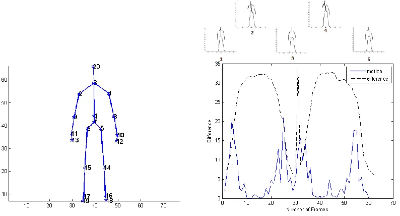
resting position are good markers for gesture boundaries. For example, Figure 8 shows a

time sequence of a user executing two gestures in a single video frame from ChaLearn

Gesture Challenge.

Figure 8: (left) The canonical skeleton used showing 20 joints, each having XYZ coordinates.

(right) Multi-gesture video sequence with 2 active gestures area (2 and 4) separated by three

non-gesture regions (1, 3 and 5). The solid blue curve is a frame to frame difference signature; the black

dotted line is frame-canonical signature. The image at the top shows the frame at the center of

non-gesture and non-gesture regions.

The solid blue line in Figure 8 is an indicator of frame to frame motion. The

motion history image (MHI). Specifically, skeletal joints per frames are converted to a

difference frame using (20). This difference frame represents the frame to frame motion.

| ) 1 , , , ( ) , , , ( | ) , ,

(x y z  g x y z f  g x y z f 

d_f (20)

where df = difference frame

f = 1,..,N-1 ; N = number of frames

g = skeleton data for a frame

The difference frame for current frame to a resting frame is given by (21).

| ) , , ( ) , , , ( | ) , ,

(x y z g x y z f r x y z

d_rf   (21)

where drf = frame-canonical difference

r = skeleton data for canonical resting frame

For (21), canonical resting image, r(x,y,z), is formulated by averaging all resting

frames of a video sequence, and serves as a reference image for comparison.

The 20 XYZ skeletal joint coordinates in each active frame are normalized akin to

a Procrustes analysis in preparation for subsequent processing using (20) and (21).

Normalization makes this technique invariant to subject distance from the camera, subject

size, and subject location within the frame. Setting s equal to a vector of XYZ skeleton

joints and c equal to a vector of XYZ canonical skeleton joints:

20 ... 1 ; 3 ... 1 / ' 1    



ij (22)

       ) ' ( ) ( ' '' s size keleton canonicalS size s

s (23)

] 20 , 7 , 4 , 3 [ ; 3 ... 1 / '' / '' '' ' 1             





s _{ij j}

n

i ij j

j

The skeleton joints are first shifted such that centroid is at (0,0,0). The size of a

skeleton is the joint to joint geodesic measure (i.e. the 3D length of the 20 blue lines in

Figure 8). After scaling, the skeleton is shifted back to the canonical skeleton location

using a centroid calculation of only the head and spine joints (joints numbered 3, 4, 7,

and 20). Omitting arm and leg joints enables the body mass to remain stationary even if a

subject's arm or leg is fully extended.

After joint normalization, the active difference signature attribute is formed by

differencing the 20 normalized skeleton joints of each frame with the 20 canonical

skeleton joint locations using (21) and with next frame using (20).

Figure 9 shows an active difference signature on the left and difference signature

on the right. Each of the 20 lines shows the temporal movement of each of the 20 skeletal

Figure 9: (left) Comparison of a displacement difference signature (left) vs. a motion

difference signature (right) for the gesture 17 from the ChaLearn dataset. Each of the line in two

figures shows the temporal displacement of one of the 20 skeletal joints from the canonical skeletal

frame (see Figure 6 for point annotation). The gesture being performed is the right hand gesture as

shown by the samples from thumbnail atop. Kinematic joints 11 and 13 showed the most

displacement from the canonical skeleton, which correspond to the right wrist and right hand

Chapter 3

Methodology

The proposed method uses only skeleton joint information from the world

coordinates (global position of tracked joints in three dimensions) as it is computationally

efficient and delivers high recognition accuracy. By incorporating ancillary information

such as RGB and depth, the training and testing time will increase significantly and thus

the system will not be useful for real time applications. Although this thesis does not

focus on making a system suitable for real time applications, it is one of the criterions

taken into account.

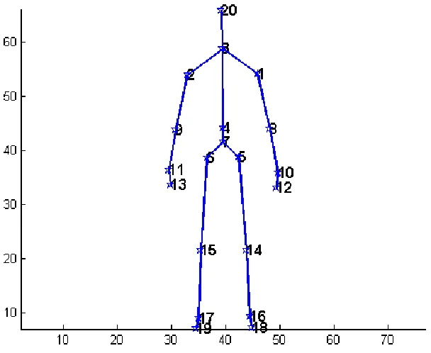
The dataset gives skeleton joint information of 20 human joints as shown below:

Figure 10: Skeleton Joints

The world coordinate is the three dimensional coordinate information of each

Figure 11 : Skelton Joint ID for ChaLearn.

For the ChaLearn dataset, the proposed method only considers movement of 13

joints out of 20 skeletal joints. This decision is based on the fact that all the gestures in

the dataset are hand based gestures, i.e. the gesture involves movement of hands only.

The joints of interest are: left hand (12), left wrist (10), left elbow (8), left shoulder (1),

right hand (13), right wrist (11), right elbow (9), right shoulder (2), head (20), shoulder

center (3), spine (4) , hip center (7), hip right (6) and hip left (5).

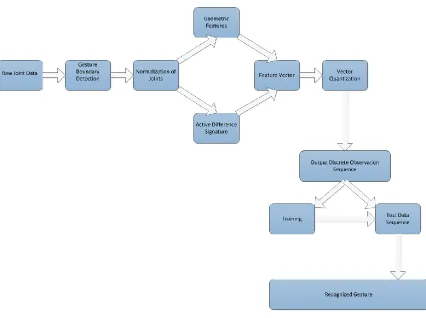
Figure 12 shows the block diagram of the gesture recognition framework. Later in

Figure 12: Gesture recognition framework.

3.1.1 Raw Joint Data

It is the raw input data from the dataset. The XYZ coordinates of all the 20

skeletal joints are input to the framework.

3.1.2 Gesture Boundary Detection

Raw skeleton joints are input to this step. Only hand joints (left hand joint - 12

and right hand joint - 13) are considered for gesture boundary detection. The rest of the

joints are discarded due to the fact that all gestures are hand based gestures. In particular,

the method considers only y-coordinates of the hand joint locations. As shown in Figure

gesture boundary, a motion filter [37] along with a space filter is used to detect these

peaks and to determine the boundaries of each gesture.

Figure 13: Hand Motion Signal. Peaks in these signals indicate a gesture in progress.

The process of segmentation using hand motion signals consists of two steps. In

the first step, the start and end frame of the gesture is identified using only one hand

(either left or right, but not both) [37]. Let N be the total number of frames in an input

gesture sequence. Let yl(i) and yr(i) be the y-coordinates of the left and right hand joint. In

the ith frame, where i = 1,2,3...,N. The value of the filter (f) for the ith frame is defined as

follows:             1 ) ( 1 1 )) ( ( , 0 ) ) ( ) ( ( , 2 )) ( ) ( ( , 1 ) (    i y y if i y i y if i y i y if i f l i r l r r l (25)

where ₁is a preset threshold that is greater than 0. A filter value of 1 indicates a

using right hand. If the filter value is zero, the corresponding frame is considered to be

such that the user is in neutral position or a gesture is performed by two hands.

The second step finds the start and end frame of the gesture performed by both

hands. This is done by computing a new adaptive threshold (₂), from the signal for each

segment with a filter value of zero. To detect gestures performed using both hands, [37]

defines a combined envelope signal as shown in Figure 14, as y_c(i)  max(y_l(i),y_r(i)).

If the value of the combined signal y_c(i)is greater than the computed threshold ₂, it is

assumed that a gesture is performed using both hands. These frames are assigned a filter

value of 3.

Figure 14: Recognition of gesture using performed using both hands. (a) Motion signals

from individual hands, (b) combined envelope signal obtained by taking the maximum value of the

individual signal at each frame, (c) filter output (normalized to one) corresponding to gesture

If a sequence of frames has a non-zero filter value, a gesture is detected, and the

start and end frames of the gestures are identified. In the post processing steps to remove

false gesture detection, a check on length of each detected gesture is performed. If the

length of the gesture is extremely short (for the ChaLearn dataset, a value of 12 is used)

then discard the detected gesture. This is done to filter away any impulse or spurious

signals (noise) that might be mistaken as a gesture. In the post processing step, another

check is also performed to check if a detected segment contains more than one gesture

(e.g. gestures that are done continuously without returning to the original or starting

position). This is done by tracking hand motion in the detected segment.

The advantage of this segmentation algorithm is that it efficiently identifies

segments containing gestures with minimal computation overhead.

3.1.3 Normalization of Joints

To prepare the data for the further processing, some basic pre-processing is

needed. Skeleton data is prone to noise and will vary with the size of the subject and

subject distance to the camera. To make joints invariant to the subject size and distance,

all frames are normalized with the canonical resting skeleton which serve as a reference

for comparison.

A canonical resting skeleton is formulated by averaging all frames of the video sequence

in which no motion is detected. The 20 XYZ skeletal joint coordinates in each active

frame are normalized akin to a Procrustes analysis. Setting s equal to a vector of XYZ

skeleton joints and c equal to a vector of XYZ canonical skeleton joints:

20 ... 1 ; 3 ... 1 /

'

1

 









i j

n s s

s

j

n

i

j

       ) ' ( ) ( ' '' s size keleton canonicalS size s

s (27)

] 20 , 7 , 4 , 3 [ ; 3 ... 1 / '' / '' '' ' 1             





s _{ij j}

n

i ij j

j

(28)

The skeleton joints are first shifted such that centroid is at (0,0,0). The size of a

skeleton is the joint to joint geodesic measure (i.e. the 3D length of the 20 blue lines in

Figure 8). After scaling, the skeleton is shifted back to the canonical skeleton location

using a centroid calculation of only the head and spine joints (joints numbered 3, 4, 7,

and 20). Omitting arm and leg joints enables the body mass to remain stationary even if a

subject's arm or leg is fully extended.

3.1.4 Geometric Features

As the ChaLearn Dataset [28] consists of only hand based gestures, only joints in

the upper body are considered for feature extraction. Specifically, the joints of interest are

the: head (he), shoulder center (sc), spine (sp), hip center (hc), left shoulder (ls), left

elbow (le), left hand (lh), right shoulder (rs), right elbow (re), right hand (rh), hip right

(hr) and hip left (hl). Geometric features are calculated only for active parts of the body,

i.e. if the gesture is performed using only right hand, then features are calculated for the

right hand only. The active body part is detected in the gesture segmentation step. Using

these joints, the following geometric features are extracted:

a) Joint Distance: For each gesture, the Euclidean distance is calculated for each of the six arm joints (hand, elbow and shoulder) with respect to head, spine and hip center

.

2 2

2 _{( ) ( )}

)

( _{j i j i j i}

ij x x y y z z

where j ϵ [he, sp, hc]

i ϵ [lh, ls, le, rh, rs, re]

As features are calculated for only active parts, the joint distance is a 9 dimensional

vector for a single hand gesture and an 18 dimensional vector for a two hand gesture.

b) Joint Angles: Joint distance can only predict whether a hand is close to the body or far from the body but it cannot differentiate between different position of the

hand in gesture space. Joint angles on the other hand can better predict position of the

joints with respect to each other. Six joint angles are calculated for each gesture. These

are shown in Figure 15 [38].

The method of calculating joint angle is illustrated in Figure 16 [38]. To calculate the

joint angle, the vector between joints must be computed. The shoulder-elbow vector

(se ) and elbow-hand vector (eh) is given by (30) and (31) respectively.

k z z j y y i x x e

s ( ₂ ₁)ˆ ( ₂  ₁)ˆ  ( ₂  ₁)ˆ (30)

k z z j y y i x x h

e  ( ₃ ₂)ˆ  ( ₃  ₂)ˆ  ( ₃  ₂)ˆ (31)

Figure 16: Calculation of elbow angle [38].

The elbow angle is given by (32).

             h e e s h e e s . arccos  (32

where the numerator, se.eh is the scalar product of the two vectors and the

denominator is the product of the magnitudes of the two vectors.

The joint angle feature vector is a 3 dimensional feature vector when the subject is

performing a single hand gesture and a 6 dimensional vector when the subject is

performing a two hand gesture as follows:



