Symmetries of unimodal singularities and complex hyperbolic reflection groups

Symmetries of Unimodal Singularities and Complex

Hyperbolic Reflection Groups

Thesis submitted in accordance with the requirements of the University of Liverpool

for the degree of Doctor of Philosophy

by

Joel Anthony Haddley

Abstract

Symmetries of Unimodal Singularities and Complex

Hyperbolic Reflection Groups

Joel Anthony Haddley

April 2011

Contents

1 Introduction 1

2 Singularities with Symmetries 3

2.1 Equivariant monodromy . . . 3

2.1.1 Symmetries and deformations . . . 3

2.1.2 Roots of the Coxeter transformation . . . 5

2.1.3 Basic equivariants . . . 6

2.1.4 Symmetric Milnor fibre and its monodromy . . . 7

2.2 The exceptional unimodal functions . . . 9

2.2.1 Classification of splitting invariant symmetries . . . 10

2.2.2 Picard-Lefschetz operators . . . 14

2.2.3 Dynkin diagrams . . . 15

2.2.4 Equivariant splitting symmetries . . . 16

2.2.5 Dynkin-like diagrams . . . 17

2.2.6 Coincidence of weights . . . 18

2.2.7 Discreteness of the monodromy group . . . 19

3 Known results 21 3.1 Lifts of simple boundary singularities . . . 21

3.2 Particular intersection numbers . . . 26

3.3 Symmetries of simple singularities . . . 27

3.4 Symmetries of P8,X9 and J10 . . . 28

3.4.1 From P8 . . . 28

3.4.2 From X9 . . . 30

4 The Classification 33

4.1 Summary of interesting results . . . 35

4.2 Classification of Invariant Symmetries . . . 43

4.2.1 E12 3x3+y7+z2 . . . 43

4.2.2 Z11 3x3y+y5+z2 . . . 45

4.2.3 E13 3x3+xy5 +z2 . . . 47

4.2.4 Q10 3x2z+y3+z4 . . . 49

4.2.5 E14 3x3+y8+z2 . . . 54

4.2.6 Z12 3x3y+xy4+z2 . . . 56

4.2.7 W123x4+y5+z2 . . . 57

4.2.8 Q11 3x2z+y3+yz3 . . . 58

4.2.9 Z13 3x3y+y6+z2 . . . 59

4.2.10 S113x2z+yz2+y4 . . . 64

4.2.11 W133x4+xy4+z2 . . . 65

4.2.12 Q12 3x2z+y3+z5 . . . 67

4.2.13 S123x2z+yz2+xy3 . . . 69

4.2.14 U12 3x3+y3 +z4 . . . 69

4.2.15 U12 3x2y+y3+z4 . . . 73

4.3 Classification of Equivariant Symmetries . . . 76

4.3.1 E12 3x3+y7+z2 . . . 78

4.3.2 Z11 3x3y+y5+z2 . . . 83

4.3.3 E13 3x3+xy5 +z2 . . . 84

4.3.4 Q10 3x2z+y3+z4 . . . 85

4.3.5 E14 3x3+y8+z2 . . . 90

4.3.6 Z12 3x3y+xy4+z2 . . . 93

4.3.7 W123x4+y5+z2 . . . 93

4.3.8 Q11 3x2z+y3+yz3 . . . 99

4.3.9 Z13 3x3y+y6+z2 . . . 100

4.3.10 S113x2z+yz2+y4 . . . 101

4.3.11 W133x4+xy4+z2 . . . 101

4.3.12 Q12 3x2z+y3+z5 . . . 102

4.3.13 S123x2z+yz2+xy3 . . . 115

4.3.15 U12 3x2y+y3+z4 . . . 120

5 Group presentations 121

5.1 Derivation of presentations . . . 121 5.1.1 2 Dimensional Groups . . . 126 5.1.2 3 Dimensional Groups . . . 131

6 Appendix 133

Chapter 1

Introduction

One of the most famous classical results in singularity theory is the Arnold and Brieskorn discovery of the close relationship between simple function singularities and Weyl groups Aµ,Dµ,Eµ [1, 6]. A few years after it, Arnold

extended the relationship to simple singularities with the _Z2 reflection sym-metry and Weyl groups Bµ, Cµ, F4.

Consideration of _Zm symmetries of simple functions led in [11, 12, 13,

22] to the appearance of Shephard-Todd groups in function singularities. The emphasis there was on realisations of the complex reflection groups as equivariant monodromy groups acting on the appropriate character subspaces in the homology of invariant Milnor fibres, and on the coincidence of the discriminants of the reflection groups and of the _Zm-equivariant functions.

A further series of papers [14, 15, 16], on cyclic symmetries of the parabolic functions, brought in similar singularity realisations of certain complex crys-tallographic groups [20].

fibre f−1(ε), and decomposes it into a direct sum of the character subspaces

Hχ, χm = 1, on which g acts as multiplication by χ. Assume the rank 2

positive subspace of the intersection form splits between two character sum-mands. Then we discover that the monodromy within a g-invariant versal deformation of f acts as a complex hyperbolic reflection group on each of the two summands. Developing further the technique introduced in papers on cyclically symmetric functions [11, 12, 13], we can construct vanishing bases in the hyperbolic summands and obtain the generating reflections as the corresponding Picard-Lefschetz operators.

The main result of the thesis is a complete classification of the symmetries of the 14 singularities, which split the positive subspace in the vanishing homology, and the description of the complex hyperbolic groups arising. The latter is done via construction of the distinguished vanishing bases in the relevant character subspaces, and via calculation of the Dynkin diagrams for such bases. All the rank 2 reflection groups obtained projectivise to the triangle groups of the Poincar´e disk, while projectivisations of some of our rank 3 groups may be found in [18].

It should be noted that it is the first time when complex hyperbolic reflection groups are appearing in a singularity theory context.

The thesis is organised as follows. Chapter 2 introduces the notion of singularities with symmetry, recalls the definitions and constructions given in [11, 12, 13], and states the exact problem we are solving in this thesis. In Chapter 3 we give an exposition of results coming from previous papers (those already mentioned as well as [14, 15, 16]), for ease of reference when consid-ering the later chapters. The classifications for the invariant and equivariant problems are given in Chapter 4. Finally, Chapter 5 discusses properties of the monodromy groups and identifies some of the low dimensional groups.

Chapter 2

Singularities with Symmetries

2.1

Equivariant monodromy

2.1.1

Symmetries and deformations

Our main object of study will be pairs (f, g) consisting of a holomorphic function germ f : (_Cn+1,0) → (_C,0) with an isolated singularity of right equivalence class X (denoted X 3 f), and a finite order automorphism g of (_Cn+1_{,0) such thatf◦g =κf, for some constant κ∈}

C. The automorphism will be called either an invariant symmetry of the function when κ = 1, or anequivariant symmetryof the function whenκ6= 1.We will not distinguish between pairs (g, κ) generating the same cyclic group acting on _Cn+1_⊕

C. Since the automorphismg is constrained by f, we may identifyg with a linear map A∈GL(n+ 1,_C). This map may be diagonalised D =P−1_AP, where matrices P−1, P may be viewed as diffeomorphic coordinate changes on (_Cn+1,0) thus preserving the right equivalence class of f.

Assume the coordinates x0, . . . , xn in (Cn+1,0) are chosen so that g is diagonal according to the previous paragraph. Consider a deformation

Fg =f + k

X

i=1

λiϕi (2.1)

of all g-equivariant (i.e. ϕi◦g =κϕi for all i) elements of a monomial basis

of the local ring Qf of f,

Qf = C

[x0, . . . , xn]

D

∂f ∂x0, . . . ,

∂f ∂xn

E.

In the standard sense, the deformationF is a g-versal deformation of f. We refer to Fg as an invariant or equivariant deformation of f (depending on

context).

All through the thesis, we use notationεm fore2πi/m, and reserveωforε3.

Example 2.1. Let f be a quasihomogeneous function of degree N with respect to the weightsw0, . . . , wn∈Nof the coordinatesxj onCn+1.Assume

gcd(w0, . . . , wn) = 1, in which case N is the Coxeter number of f. Consider

the Coxeter transformation

C : xj 7→ε wj

N xj, j = 0, . . . , n,

of _Cn+1_{. This is an invariant symmetry of f. The Coxeter element C} gen-erates a discrete subgroup of U(1) corresponding to the values of f making one full anti-clockwise rotation in _C about the origin. Take for an invariant symmetry g of f a power of C that has order m: g = Cp_{, g}m _{= id. Then}

the ϕi in (2.1) are exactly those elements of a monomial basis of Qf whose

degrees are divisible by m.

In the equivariant case, suppose the deformation monomial of minimal degree ϕ0 has degree d0. Then the symmetry g on the meromorphic function

f /ϕ0 is invariant, and theϕi in 2.1 are exactly those elements of a monomial

basis of Qf whose degrees d are such that (d−d0) is divisible by m. This

generalisation also holds for the invariant case since the constant monomial is of degree 0 (cf. [22] and [23]).

These are the only elements of a monomial basis forQf with weights divisible

by 7 (see Table 2.1 on page 11).

We shall use the notation Λ for the base _Ck with coordinates λ1, . . . , λk

of a g-miniversal deformation (2.1) of a function f.

Definition 2.3. The discriminant Σ⊂Λ of f is the set of all values λ ∈Λ of the parameters for which the members of the family Fg have critical value

0.

For a versal deformation (i.e. take g to be the identity) the deformation Fg

at a generic pointλ∈Λ has no critical point with value 0 and its derivatives are smooth. This is not necessarily true when g is not equal to the identity map, and the following definition is required in order to maintain this generic behaviour.

Definition 2.4. A deformationFgis said to besmoothableif the discriminant

Σ⊂Λ is a hypersurface.

Since for an invariant deformation a non-zero constant function must be among the ϕi, the deformation is smoothable.

Proposition 2.5. If an equivariant deformation is smoothable, then at least one of the ϕi must be linear.

Proof. Assume otherwise. Then the ϕi of lowest degree must be at least

quadratic, and for any λ ∈ Λ there is a critical point at the origin of _Cn+1 on the zero level.

In what follows we will be working with representatives of germs of functions and sets we have introduced, but we will be still denoting them by the same letters.

2.1.2

Roots of the Coxeter transformation

For a singularity X 3 f, let C be the Coxeter transformation of order N

given in coordinates by

where α/a = wx0/N is the weight of x0, normalised so that the weight of f

is wf = 1. Take the canonical choice for the root

(εa)

1

s :=ε as,

which we apply to each coordinate in turn to define the map

C1s(x₀, . . .;f) = (εα

asx0, . . .;εsf).

The map C1s and each of its powers gives an equivariant symmetry of f.

Consider the bth _power

Cbs = (εαb

asx, . . . , ε b sf),

where we may choose b such that gcd(b, s) = 1, since we otherwise would have chosen a different value for s.

By proposition 2.5, any smoothable equivariant deformation has a linear term in its deformation. Assume without loss of generality that this is the monomial x0. Then

εαb_as =εb_s.

For this equality, we must choose b such that a|b. Since N is the Coxeter number, we generate all possible non-equivalent equivariant symmetries by letting b run through all divisors of N such that if bi and bj are two choices

for b, then bi andbj have pairwise distinct greatest common divisors withN

for all i6=j. We may then find other equivariant symmetries by changingn. The order of the symmetry is m =sN/b.

2.1.3

Basic equivariants

Definition 2.6. If g is an equivariant symmetry of the function f such that the monomial x0 appears in the g-versal deformation, then it is an invariant symmetry of the meromorphic function f /x0. We choosegx0 to be

a symmetry of this type of highest order, and call gx0 the basic equivariant

of f with respect to x0. If we find gx =C

b

b, s, then we may use the argument above to classify all equivariant defor-mations of f preserving x0.

Most of the invariant symmetries that will appear in our consideration are the involutions

ιI :xi 7→

(

xi, xi 6∈I

−xi, xi ∈I

where I ⊆ {x0, . . . , xn} is a subset of the coordinates. E.g.

ιx(x, y, z) = (−x, y, z).

Example 2.7. For E12 3 f = x3 +y7 +z2, the Coxeter transformation is given by

C(x, y, z;f) = (ωx, ε7y,−z;f).

The basic equivariant gx in an invariant symmetry of highest order of the

meromorphic function f /x =x2+y7/x+z2/x.We may take

gx(x, y, z;f) = (−x, ε143 y,−iz;−f),

and we have

gx =C

3 2.

2.1.4

Symmetric Milnor fibre and its monodromy

provided λ is non-discriminantal (λ ∈ Λ\Σ). In good cases, for example when the function is quasihomogeneous with positive weights, we may expand our deformation representative from the product of the balls to the whole

Cn+1×Λ. For more details see [5], Sections 1.7 and 1.10.

Let us fix a generic point?∈Λ\Σ. The Milnor fibre V? is homotopic to

sends V? into itself. Therefore, its nth homology, of total rank µ, is a direct

sum of character subspaces

Hn(V?,C) = ⊕χm₌₁H_χ, (2.2)

where mis the order of the automorphismg, andg acts as multiplication by

χ on Hχ.

There is a standard way to define elements of the Hχ analogous to the

ordinary Morse vanishing cycles. Namely, let W be the quotient of the fibre

V? by the action of the group Zm generated by g, and W0 ⊂ W its subset

of irregular orbits. Since all functions Fλ in the family F are g-invariant

(or equivariant depending on context), a path in Λ \Σ from the point ?

to a generic point of the discriminant defines - at least in all our cases - a vanishing cycle σ ∈ Hn(W, W0;Z): similar to what has been observed and

used in [2, 11, 12, 13], in all our cases it is easy to see a generator of the relative integer homology which contracts to a point on the approach to the discriminant. The inverse image of this relative cycle in V? consists of m

chains σ0. . . , σm−1,with the orientation inherited from σ,and ordered in the cyclic way:

g(σi) = σ(i+1) modm.

For appropriate values of χ(the notationχdenotes its conjugate), and in all the cases which will follow, the linear combination

σχ= m−1 X

i=0

χiσi

is a cycle, and thus provides an element ofHχ.We callσχavanishingχ-cycle.

See Figure 2.1. Examples of these calculations are given in Chapter 3. The monodromy representation of the fundamental group π1(Λ\Σ, ?) on

Hn(V?,C) is a direct sum of the representations on the individual summands

Hχ. We denote the corresponding monodromy groups Mχ.

χ−1 1

χ

g

quotient map

χ−1 1

χ g

quotient map

W σ _W0 σ

V? V?

Figure 2.1: Diagram showing χ-cycles as cyclic covers of chains.

that a vanishing χ-cycle σχ has a non-zero self-intersection number hσχ, σχi.

Then according to [4, 8, 11] the related Picard-Lefschetz operator inMχ may

be brought into the form

hχ: c7→c+ (e−1)

hc, σχi

hσχ, σχi

σχ,

where e is the eigenvalue of the operator on σχ. This is a (skew-)Hermitian

reflection on Hχ.

To obtain a generating set of theMχ, we proceed in the traditional

man-ner. For this, we start with a generic line L ⊂ Λ passing through the base point?. Letc1, . . . , cr be the points at whichLmeets Σ. We choose a

distin-guished system of paths onL, that is, pathsγ1, . . . , γr inL, starting at?and

leading to the ci, which have no self- and mutual intersections except for the

point ?itself. The Picard-Lefschetz operators hi,χ on the Hχ corresponding

to the paths of the system generate Mχ. Thus knowledge of the

eigenval-ues of the hi,χ and of the intersection numbers of the χ-cycles vanishing at

c1, . . . , cr yields a description of the monodromy groupMχ.

2.2

The exceptional unimodal functions

Now assume that f is one of the 14 exceptional unimodal singularities and

quasihomogeneous member of each of the 14 one-parameter families, along with the weights of the coordinates, the Coxeter number N, a monomial basis of the local ring and the weights of its elements. The subscript of the singularity right equivalence type it the Milnor number µof the singularity. Pairs of functions with the same Coxeter number are dual in the sense of Arnold. Any function with µ= 12 is self-dual.

An arbitrary member of a unimodal family is obtained by addition to the normal form of a multiple of its Hessian, that is, of a multiple of the versal monomial of top weight.

Assume we have two coordinate spaces, _Cp_u1,...,up and _Cq_v1,...,vq, with co-ordinates of positive integer weights a1, . . . , ap and b1, . . . , bq. Then the

space of map-germs from (_Cp_{,0) to (}

Cq,0) has a natural grading: a mono-mial summand uα1

1 . . . u

αp

p in the jth coordinate function is assigned grading

α1a1+· · ·+αpap−bj. For example, a quasihomogeneous automorphism g of

Cp has all its monomial terms of grading 0. The determinant J ac(g) of the Jacobi matrix of such automorphism is a non-zero constant, which is easily seen if the coordinates are ordered by the increase of their weights.

In what follows, we are restricting our attention to quasihomogeneous symmetries of exceptional unimodal singularities.

2.2.1

Classification of splitting invariant symmetries

reflec-tion groups, that is, the restricreflec-tion of the intersecreflec-tion form to the summand

Hχ is non-degenerate and of positive signature 1. Hence the rank 2

posi-tive subspace H+ ⊂ H2(V?,C) must split between two character subspaces

Lemma 2.8. Assume symmetry g is quasihomogeneous. Then g is splitting if and only if J ac(g)∈/ _R. In this case, the hyperbolic characters are J ac(g) and its conjugate.

Proof. According to [24], the rank 2 subspace in the cohomology H2_(V

?,C)

dual to H+ is spanned by the forms α = dx∧dy∧dz/dF? and Hess(f)α.

The two forms are eigenvectors of the automorphism g? _{of H}2_(V

?,C), with

the eigenvalues J ac(g) and its conjugate.

Corollary 2.9. Non-quasihomogeneous exceptional unimodal functions have no splitting symmetries.

Indeed, a symmetry of such a function preserves the modular termHess(f). Hence both α and Hess(f)α are in the same character subspace in the cohomology.

Our main classificational result, on normal forms of splitting symmetries, is

Theorem 2.10. Any invariant splitting symmetry g of a quasihomogenous exceptional unimodal singularity f falls into one of the following categories. a) The symmetry g of order m >2is a power of the Coxeter

transforma-tion C of function f.

b) Each of the corank 2 singularities E14, Z13, W13, W12 admits symme-tries g of order m >2which are powers of the Coxeter transformation composed with the involution ιz(x, y, z) = (x, y,−z).

c) Remaining symmetries are listed in Table 2.2.

Table 2.2 lists the symmetries up to a choice of a different generator of the same cyclic group.

The involution ιx used in Table 2.2 has been introduced in Section 2.1.3.

Table 2.2: Exceptional symmetries of Q12 and U12

f g :x, y, z 7→ g = |g| g−miniversal

monomials notation

Q12: x2z+y3+z5 ε910x, ωy, ε5z ιxC 30 1 −

ιx : (x, y, z)7→ ε710x, y, ε35z ιxC3 10 1, y Q12|Z10 7→(−x, y, z) −x, ω2_{y, z ι}

xC5 6 1, z, z2, z3, z4 Q12|Z6

U12 : x3 +y3+z4 ω2x, y, iz σC 12 1, y U12|Z12

σ: (x, y, z)7→ x, ωy,−z σC2 _{6 1, x, z}2_{, xz}2 _U 12|Z6 7→(ωx, ω2_{y, z) ωx, ω}2_{y,−iz σC}3 _{12 1, xy (U}

12|Z12)0

ω2x, y, z σC4 3 1, z, y, z2, yz, yz2 U12|Z3

U12: x2y+y3+z4 ε56x, ωy, iz ιxC 12 1 −

ιx : (x, y, z)7→ ε6x, ω2y,−z ιxC2 6 1, z2 (U12|Z6)0 7→(−x, y, z) −x, y,−iz ιxC3 4 1, y, x2, xz2 (U12|Z4)0

ε5

6x, ωy, z ιxC4 6 1, z, z2 (U12|Z3)0

ιx

ιx

σ

the corresponding power of the Coxeter transformation. For the corank 2 functions not mentioned in part b), the symmetry (x, y, z) 7→ (x, y,−z) is

CN/2_.

Theorem 2.10, in particular, states that, for any quasihomogeneous excep-tional unimodal singularity f, we can make a quasihomogeneous coordinate change which diagonalises a splitting symmetry. In the case of U12, there are two possible normal forms. This is similar to the two normal forms of the

D4 singularity.

The sign change in part b) of the Theorem is the−idmap on the vanishing homology. It does not affect the actual summands in the decomposition (2.2). It only affects the indexation, changing the signs of all characters.

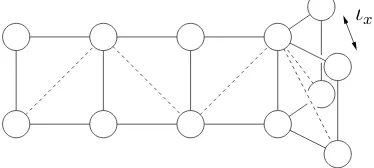
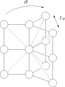
The transformations ιx and σ in Table 2.2 correspond to the order 2

and 3 symmetries of the Dynkin diagrams of the underlying singularitiesD6 and D4. The relevant symmetries of the Q12 and U12 Dynkin diagrams are shown in Figure 2.2 (the diagrams are constructed as those for the direct sumsD6⊕A2 and D4⊕A3 of singularities, using the Gabrielov method [10]). Both ιx and σ have real determinants, hence are able to split the subspace

H+ only in combination with a power of the Coxeter transformation which splits H+ itself, that is, has order greater than 2.

2.2.2

Picard-Lefschetz operators

Since the character J ac(g) has a special role, we will use a special notation

χ0 for it. In the direct sum

H2(V?,C) =⊕χm₌₁Hχ, (2.3)

where the substitution g? is multiplication by χ on Hχ, we have α = dx∧

dy∧dz/dF? ∈ Hχ 0

. Each summand Hχ _{here is dual to the summand H} χ in

(2.2).

Proposition 2.11. Consider the Picard-Lefschetz operator hχ0 onH_χ0

corre-ponding to a g-orbit of critical points with a quasihomogeneous normal form

ψ(x0, y0, z0). Choose the weights w₁0, w0₂, w₃0 of the variables so that the weight of function ψ is 1. Then the eigenvalue of hχ0 is exp(2πi(w0

1+w

0

2+w

0

3)). Proof. The restriction of the familyF to a line germ transversal to Σ may be brought near any of the critical points to a local normal formψ(x0, y0, z0) +. Locally, the cohomological operator h? _{= ⊕h}χ _{is induced by a loop in}

C

going once around the origin in the positive direction. Its eigenvectors are the 2-formsωj =αj(x0, y0, z0)dx0∧dy0∧dz0/dψ, where theαjform a monomial

basis of the local ring of functionψ. The transformationh? is the substitution

x0 := exp(2πiw0₁)x0 etc. Hence its eigenvalue on ωj is exp(2πi weight(ωj)),

where weight(ωj) =weight(αj) +w01+w

0

2+w

0

3.

The only eigenformωj that vanishes nowhere in a neighbourhood of our

elementary critical point is the one in which αj is a non-zero constant, that

is, has weight 0.

2.2.3

Dynkin diagrams

Our classification is encoded in the standard way using Dynkin diagrams. One interpretation of these diagrams gives a description of the structure of the discriminant Σ ⊂ Λ. Another interpretation we use says that a vertex corresponds to a generator of π1(Λ\Σ) (equivalently Mχ), and the edges

correspond to some of the relations. This part of the relations will be denoted by B. Both interpretations are presented in Table 2.3. While we don’t necessarily find a two dimensional section of the discriminant in each case, this interpretation still holds.

The exterior of each vertex is also labelled with the right equivalence class of the function germ corresponding to this component of the discriminant. The eigenvalue of the Picard-Lefschetz operator corresponding to the vertex coincides with the eigenvalue of the classical monodromy of this function germ, and the order of this is written in the interior of the vertex. This is the order of the generator of Mχ0 corresponding to this vertex.

of the vanishing χ-cycle associated to this generator, and edges with the intersection numbers of neighbouring χ-cycles. The intersection number is zero if and only if there is no edge between vertices. See page 22, for example.

Table 2.3: Dynkin diagram relations on pairs of vertices

Singularity Dynkin diagram Local structure of Σ B-relations

A1×A1

s t

st=ts

A2

s t

sts=tst

B2

s t

(st)2 = (ts)2

G2

s t

(st)3 _{= (ts)}3

2.2.4

Equivariant splitting symmetries

Similar considerations can be made in the equivariant case by also considering constant multiples of the functions itself. We have the following classification theorem.

Theorem 2.12. Any smoothable equivariant splitting symmetryg of a quasi-homogeneous exceptional unimodal singularityf falls into one of the following categories

a) The symmetry g of order m > 2 is a fractional power of the Coxeter transformation C of function f.

b) Each of the corank 2 singularities E14, Z13, W13, W12admits symmetries

c) Remaining symmetries are powers of C composed with an invariant symmetry ιx or σ (shown in Figure 2.2) which will be discussed in

detail for Q12 on Page 102 and U12 on Page 117.

2.2.5

Dynkin-like diagrams

For equivariant symmetries, we recall a definition stated in [7]:

Definition 2.13. A group with ` generators acting on _Ck _{is called well}

presented if k =`.

By convention, we draw the Dynkin diagram of a group with a ‘curved edge’ if and only if it is not well presented.

Definition 2.14. Such a diagram is called aDynkin-like diagram, the 3-wise relations are called braid-like.

In [7] as well as in this thesis we find that the largest observed`is`=k+1 (in the equivariant case only). Such groups may have generators which satisfy braid-like relations. All such relations necessary for this thesis can be found in Table 2.4 on Page 18, along with the Dynkin-like diagrams encoding these relations.

The diagrams given in Chapter 3 correspond to the same groups as those in Goryunov’s papers, but in some cases may look different. Due to the amount of labelling frequently required, we introduce a new notation – that of the intersection diagram. If there is insufficient room to properly label a Dynkin diagram, it is followed by an intersection diagram containing all nec-essary information about intersection numbers. These diagrams have black vertices to distinguish them from Dynkin diagrams.

Table 2.4: Dynkin-like diagram relations on triples of vertices Dynkin diagram Local structure of Σ B-relations

s

u

t

s

u t ?

stu=tus=ust

t

u

s

s

u t ?

sutst =utsut, utsu =suts

s

t

u

s

u t ?

ustut=tustu, stu =tus

2.2.6

Coincidence of weights

Definition 2.15. The graph obtained by removing all labels and orders of vertices of the Dynkin diagram is the skeleton of the Dynkin diagram. As in Example 2.1, we takef to be a quasi-homogeneous function of degreeN

with respect to the weightsw0, . . . , wnof the coordinates wherew0, . . . , wn∈

N, gcd(w0, . . . , wn) = 1. Choose the weights v1, . . . , vk of λ1, . . . , λk in the

unique way so that

Fg =f + k

X

i=1

λiϕi

is quasi-homogeneous, and assume they are arranged so thatvi ≤vi+1 for all

i= 1, . . . , k−1.

Similarly, let G be a finite reflection group acting on _Ck _{(as classified}

in [21]), basic invariants of which have degrees m1, . . . , mk also arranged so

Definition 2.16. A group with`generators acting on akdimensional vector space is said to have corank`−k.

Proposition 2.17. Let Mχ0 be a complex hyperbolic reflection group in our

classification, andv1,· · ·, vk the weights of the parameters in a corresponding

g-miniversal deformation. Assume the ratio (v1 :· · ·:vk) coincides with the

ratio (m1 :· · ·:mk) of degrees of basic invariants of a Shephard-Todd group

G. If Mχ and G have equal coranks, then Mχ0 and G have Dynkin diagrams

with coinciding skeletons.

Conversely, coincidence of the skeleton of a Dynkin diagram ofMχ0 with

that of some Shephard-Todd group G implies the equality of the weights ratio of Mχ0 and the degrees ratio of G.

2.2.7

Discreteness of the monodromy group

We recall the following. Let H be an Hermitian form, and consider an algebraic number field E such there exists a totally real subfield F with [E : F] = 2. Use OE to denote the ring of integers of E. Let SU(H) denote

the special unitary group defined by the form H, and SU(OE, H)⊂SU(H)

be the subgroup consisting of matrices with entries belonging to OE. There

are a finite number of embeddings ρi : F → R. For each of these

embed-dings there is, up to complex conjugation, a unique compatible embedding

τi :E → C,from which we obtain a new Hermitian matrix τjH by applying

τj to the entries of H. The new associated group SU(τjH) is denoted by τj_SU(H).

Theorem 2.18(Deligne, Mostow [9]). The subgroupSU(OE, H)is an

arith-metic lattice in SU(H) if and only if τj_{SU(H) is compact for all non-trivial}

embeddings τj (up to complex conjugation).

Corollary 2.19. The projectivised versions of all groups appearing in the following classification are discrete subgroups of SU(k−1,1).

After taking the quotient of the Milnor fibre by the symmetry group gener-ated by g the group is the direct sum of groups, each of dimension kχ ≤ k

(by observation).

M = M

χ:χm₌₁

Mχ.

Due to Lemma 2.8, we assume χ0 6∈ _R. Let χ0 (and therefore its conjugate) be such that Mχ0 ⊂U(k−1,1).Since the sum of signatures of the character

subspaces must equal the signature of their direct sum, for all χ 6= χ0 (up to complex conjugation) we have Mχ ⊂ U(kχ), which is compact. After

projectivisation the compactness argument also holds, and moreover entries in the matrices belong to the cyclotomic ring _Zhχi. The field _Qhχi is an imaginary quadratic extension of the totally real subfield_Qhχ+χisince the minimal polynomial of χ in _Qhχ+χi is

x2−(χ+χ)x+ 1.

Chapter 3

Known results

This chapter gives all results coming from other papers which are used in the classification in Chapter 4.

3.1

Lifts of simple boundary singularities

We recall all results from [11, 12, 13] relevant to this thesis.

Example 3.1. The boundary singularity A2 has normal form x3 +y0+z2, boundary given by {y0 = 0}. We take an m-fold covering of C3 ramified along the boundary by settingy0 =ym.This is similar to taking a singularity

X 3x3 +ym+z2 of codimension 2(m−1), and considering X|_Zm with the

symmetry g : (x, y, z) 7→ (x, εmy, z). We consider the picture without the

variable z.

V

0 a

b y0 _Vˆ y

1 1

χ χ y0=ym

→

Figure 3.1: Taking m-fold covers of semi-cycles a and b.

the homology of the Milnor fibre of A2 in the standard way as described in Section 2.1.4. We use ˆV to denote the boundary cover of the Milnor fibreV by the substitutiony+ 0 =ym_{. Figure 3.2 shows that}D_{(1−χ)ˆa,ˆb}E_=m,where

the solid paths are obtained by multiplying the solids paths corresponding to ˆa in Figure 3.1. The suspension of cycles into an extra dimension by adding the variablez2 _{implies self-intersection number−mfor both ˆa,}ˆ_b.The intersection form is Hermitian for an odd number of variables, which also gives for 3 variables

D ˆ

a,ˆbE= m 1−χ.

1 1

χ χ

Figure 3.2: Proof thatD(1−χ)ˆa,ˆbE=m.

The intersection matrix is therefore

−m − m χ−1 − m

χ−1 −m !

,

whereχm _{= 1, χ6= 1.The function germ representative corresponding to the}

only component of the discriminant is of right equivalence class Am−1. The eigenvalue coming from the classical monodromy of this is of order dividing

m. We want our groups to be hyperbolic, giving the constraint |χ−1|<1, so we must take χ = εm or χ =εm if 6 < m < 13. So we get the following

diagram for A(₂m).

Am−1 m Am−1

εm−1

m m

−m −m

Pairs of connected vertices in the Dynkin diagram for a singularity of type

Aµ(m), D(µm), Eµ(m) have the same local structure as A(2m), and the labelling for each pair is the same as in the diagram above.

An ambiguity occurs when we label cycles with powers of χ (e.g. see Figure 3.1) since we could start this labelling process on any cycle, and when we choose orientations. For this reason, the intersection number of the two cycles is defined only up to multiplication by a power of εm or by ±1. It is

shown in [11] that adding a non-degenerate quadratic form in an even number of variables to a function affects the intersection numbers only perhaps by further multiplication by −1. Moreover, if the Dynkin diagram is a tree this ambiguity affects every edge and we have freedom to choose the most convenient intersection number.

Oriented edges of Dynkin diagrams indicate the order in which we take intersection numbers:

a→U b,

means ha, bi=U. However the reorientation

a ←U b

may easily be brought to the form

a ←U b

by the ambiguities mentioned in the previous paragraph. So in the case when the Dynkin diagram is a tree (specifically this example), we do not assign orientations to the edges of the diagram.

Example 3.2. Starting with the boundary singularity B2 3 y02 ({y0 = 0} the boundary) and setting y0 = ym, we obtain the singularity B

(2,m) 2 . To construct its diagram we use an explicit example as in [11]. Consider the covering y0 = ym of a deformation f(y0) = y20 −4y0 + 3 of the one variable boundary singularity B2. Set ˆf(y) = f(ym). Take ˆf = 0 as the Milnor fibre

b

points on the inner circle in Figure 3.3 for a χ−cyclee1 ∈Hχ⊂H0(Vb) (the reduced 0-degree homology) vanishing on the level ˆf = 3,and the difference between the linear combinations on the outer and inner circles for a χ−cycle

e2 vanishing on ˆf =−1. The intersection matrix (hei, eji) is

m −m

−m 2m

!

.

0 1 1

χ χ χ−1

χ−1 2π/m

Cz

Figure 3.3: Cycles for B2

The Picard-Lefschetz operator h1 rotates the points on the inner circle anti-clockwise by 2π/m which means

h1(e1) = χe1,

h1(e2) = e2+ (1−χ)e1

= e1−(1−χ)he2, e1ie1/m = e1+ (χ−1)

he2, e1i he1, e1i

e1.

The operator h2 swaps points on the same ray from the origin:

h2(e1) = e1+e2

= e1− he1, e2ie2/m = e1+ (e2πi/2−1)

he1, e2i he2, e2i

e2,

h2(e2) = −e2.

Am−1 m mA1

m 2

−m −2m

Together with the result for A(₂m), we may now construct Dynkin diagrams for similar lifts of all simple boundary singularities. In each case there are µ

vertices. Dashed edges in the following diagrams indicate the diagram should be continued by a chain of vertices.

Am−1 Am−1 Am−1 Am−1 Am−1

m m m m m

m εm−1

m εm−1

m εm−1

−m −m −m −m −m

A(µm)

Am−1

Am−1

Am−1 Am−1 Am−1 Am−1

m

m

m m m m

m ε8−1

m εm−1

m εm−1

m εm−1 −m

−m

−m −m −m −m

D(µm)

Am−1 Am−1 A_m−1

Am−1

Am−1 Am−1

m m m

m

m m

m εm−1

m εm−1

m εm−1

m εm−1

−m −m −m

−m

−m −m

Am−1 mA1 mA1 mA1 mA1

m 2 2 2 2

m m m

−m −2m −2m −2m −2m

Bµ(m)

mA1 Am−1 Am−1 Am−1 Am−1

2 m m m m

m _εmm_{−1 εm}m₋₁

−2m −m −m −m −m

Cµ(m)

Am−1 Am−1 mA1 mA1

m m 2 2

m

εm−1 m m

−6 −3 −6 −6

F₄(m)

From now on, we will choose the special character χ0, the eigenvalue of g?

on dxdydz_df , details of which are given in Section 2.2.1, so that the monodromy group in our case is complex hyperbolic.

3.2

Particular intersection numbers

In [12], a series of invariant singularities

Dm+1|Z2m 3 x2y+ym+z2;

g(x, y, z) = (ε2mx, εmy, z)

was introduced. The self-intersection number of theχ-cycle e corresponding to this singularity ishe, ei=m(−2 +χ+χ),χm =−1. In particular, we will use the following with χ=ε2m:

• For D5|Z8, he, ei= 4(−2 +ε8+ε8) = 4 √

2−8,

• For D6|Z10,he, ei= 5(−2 +ε10+ε10) = 5₂( √

5−3).

We also need the self-intersection number of a χ−cyclee corresponding to a singularity of type E6|Z12, χ=−iω=ε12. According to [19], this is

he, ei=−2·3·4 1−(−1)·ω·i

(1−(−1))(1−ω)(1−i) = 2 √

3−6.

3.3

Symmetries of simple singularities

Full details of the following singularities with invariant symmetry are given in [12], the singularity with equivariant symmetry in [13].

B₂(4)

For f = x8 +yz ∈ A7 with the invariant symmetry g(x, y, z) = (ix, y, z),

g-versal monomials are 1, x4 _{and the Dynkin diagram is given.}

A3 ₄ 4A1

4 2

−4 −8

A group with the same notation occurs as a symmetry of D5. Namely, for

f =x2_y+y4_+z2 _{with the invariant symmetry g(x, y, z) = (−ix, y,−z), g} -versal monomials are 1, y2_{, and the Dynkin diagram is given.}

A3 ₂√₂ 2A1

4 2

−4 −4

B₂(3,3)

Forf =x3+y4+z2 ∈E6with the invariant symmetryg(x, y, z) = (ωx,−y, z),

g-versal monomials are 1, y2 and the Dynkin diagram is given.

A2 6 2A2

ω−1

3 3

B₂(4,3)

For f = x3 + y5 + z2 ∈ E8 with equivariant symmetry g(x, y, z;f) = (−ωx,−y, iz;−f), g-versal monomials are y, y3 and the Dynkin diagram is given.

D4 6 2A2

ω−1

4 3

−61− ε512

ω−1

₋₆

3.4

Symmetries of

P

,

X

and

J

Here we display some of known Dynkin diagrams of groups coming from sym-metries ofP8,X9 andJ10 which can be found in [14, 15, 16] respectively. We fix the character such that these groups are complex crystallographic reflec-tion groups, and extending these groups in our classificareflec-tion yields complex hyperbolic reflection groups. We omit some of those groups which are iso-morphic to ones already mentioned in this chapter.

3.4.1

From

P

The following results come from [14].

C₃(3,3)

For f = x3 + y3 + yz2 ∈ P8 with the invariant symmetry g(x, y, z) = (ωx, y,−z), g-versal monomials are 1, y, y2 and the Dynkin diagram is given.

2A2 A2 A2

3 3 3

2(1−ω) 1−ω

−6 −3 −3

(P8|Z6)0

For f = x3 _{+ y}3 _{+ yz}2 _{∈ P}

D4 ₃ D4

6 6

−3 −3

C₂(2,4)

For f = x2z + xy2 +z3 ∈ P8 with the invariant symmetry g(x, y, z) = (−x,−iy, z), g-versal monomials are 1, z, z2 and the Dynkin diagram is given.

2A1 A3 A3

2 4 4

2(1−i) 2(1−i)

−4 −4 −4

P8/Z6

For f = x3 _+y3 _+z3 _{∈ P}

8 with the equivariant symmetry g(x, y, z;f) = (−ωx,−y,−z;−1), g-versal monomials are y, z and the Dynklike and in-tersection diagrams are given.

2A2

2A2

2A2 3

3

3

−6

−6

−6

−6

−6

−6

P8/Z4

For f = x2_{z +xy}2_+z3 _{∈ P}

2A1

4A1

A3 2

2

4

−4

−8

−4

−4(i−1)

−4 4(i−1)

3.4.2

From

X

The following results come from [15].

B₂(6,3)

For f = x4 + xy3 + z2 ∈ X9 with the invariant symmetry g(x, y, z) = (−x,−ωy, z), g-versal monomials are 1, x2 _{and the Dynkin diagram is given.}

A5 ₆ 2A2

6 3

−6 −6

X9/Z6

The paper [15] does not use Dynkin-like diagrams, so we perform our own calculations. For f = x4 +xy3 +z2 ∈ X9 with the equivariant symmetry

g(x, y, z;f) = (ωx, ωy, ωz;ωf). We have

Fg = x4+xy3+z2+γx2y+βy2+αx

Fg,x = 4x3+y3+ 2γxy+α

The first two components of the discriminant are Σ1 = {α = 0} and Σ2 = {27α2+γ3α−16β3−36γβα+8γ2β2−γ4β}. The union Σ1∪Σ2is a standardB3 type discriminant. The final component Σ3 ={β = 0}gives a line producing a triple point in a generic section. All other intersections are transversal. The Dynkin-like and intersection diagrams follow.

3A1 3A1

A3 3A1

2 2

3 2

−6 −6

−3 −6

3

3 3ω u

3ω

u= 3(1−ω)

3.4.3

From

J

The following results come from [16].

J10|Z3

For f = x3 _{+ y}6 _{+ z}2 _{∈ J}

10 with the invariant symmetry g(x, y, z) = (ωx, ωy, z), g-versal monomials are 1, y3_{, xy}2 _{and the Dynkin diagram is} given.

3A1 D4 3A1

2 6 2

3 3

C₃(4)

Forf =x3+xy4+z2 ∈J10with the invariant symmetryg(x, y, z) = (x, iy, z),

g-versal monomials are 1, x, y4 and the Dynkin diagram is given.

4A1 A3 A3

2 4 4

4 _i−4₁

−8 −4 −4

J10/Z4

For f = x3 +xy4 +z2 ∈ J10 with the equivariant symmetry g(x, y, z;f) = (−x,−y, iz;−f), g-versal monomials are y, y3, y5, x, xy2 and the Dynkin-like diagram is given.

2A1 2A1 2A1 2A1 2A1 2A1

2

2 2 2

2 2

−4 −4 −4 −4

−4 −4

2 2 2

2 2

2(i+ 1)

u u

Chapter 4

The Classification

In this chapter we list all splitting symmetries of the 14 exceptional unimodal singularities given in Table 2.1. Each symmetry is presented with an accom-panying Dynkin (or Dynkin-like) diagram encoding all necessary information to describe the monodromy subgroup with hyperbolic signature. When con-sidering a singularity of right equivalence classX with respect to a symmetry

g of order m, we write X|_Zm in the invariant case, X/Zm in the equivariant

case, or one of these with dashes to distinguish between symmetries of the same order with different g-versal deformations. Some lifts of simple singu-larities are already well known in the literature, for others we may use the following shortcuts in calculation.

1. IfX|_Zm →Y|Zm with the same symmetryg then the Dynkin diagram

of Y|_Zm is a sub-diagram of some Dynkin diagram of X|Zm. In the

cases Y is one of the parabolic singularities P8, X9, J10,the details can be found in [14, 15, 16] respectively; if Y is a simple singularity the details can be found in [11, 12, 13]. All relevant information from these papers is reproduced in Chapter 3 and specific parts will be referenced as we proceed.

2. The following may occur. Let X admit an orderm symmetry g where

g(zi) = zi. If X also admits an order 2m symmetry g0, defined by

g0(zi) = −zi and g0(zj) = g(zj) such that Fg 6≡ Fg0, then the Dynkin

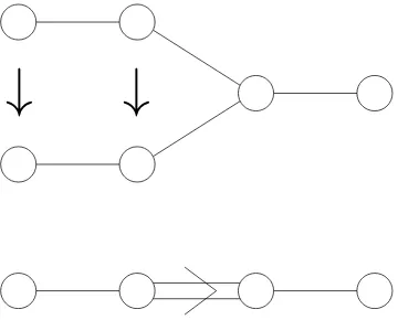
usual sense. For example, take E6 3 f = x4 +y3 +z2 with g = id, a trivial symmetry, and g0(x, y, z) = (−x, y, z) of order 2. Then the normal form E6|Z2, i.e. after the substitutionx2 =x0, isx20+y3+z2 ∈

F4.ThereforeE6|Z2 =F4,and this is demonstrated visually by folding the Dynkin diagram. See Figure 4.1.

3. It is not necessary to calculate unknown intersections geometrically. Say our Dynkin diagram forX|_Zm is fully labelled except for an

inter-section number U of two particular cycles. We may write the matrices of our Picard-Lefschetz operators in terms ofU, and observe that these should satisfy certain braiding relations. These give a condition on |U|2_{. We further observe that U ∈}

Zhχ0i. We write a general element of this ring and impose the value of |U|2_{. This usually gives a system} of diophantine equations with lcm(2, m) solutions which we calculate by brute force using the MAPLE code given in Section 6.1.

4. In the invariant case, the Milnor numberµofXis preserved as the sum of multiplicities of singularities corresponding to intersection points of the discriminant with the generic line. We will refer to this as Σµi =µ

in what follows. A similar equivariant constraint will be discussed later.

↓

↓

Symmetries are given only up to coinciding symmetric versal deformations. We do not include symmetries of order 2 since by Lemma 2.8 we require the eigenvalue of g not to be real.

In each case, we assume the symmetryghas the standard formg(x, y, z) = (ax, by, cz), where a, b, c are to be found. Solving f ◦g(x, y, z) = f means solving a system of three equations in a, b, c, written

aαibβicγi = 1, i= 1,2,3.

Here α1, β1, γ1 are exponents in the monomial summand xα1yβ1zγ1 of the singularity. The absolute value of the determinant of the matrix of exponents

∆ =

α1 β1 γ1

α2 β2 γ2

α3 β3 γ3

gives the number of solutions to this system. If ∆ = N, the order of the Coxeter elementC, then all solutions, and therefore all symmetries, must be powers of C. If the number of solutions to this system is equal to 2N and the function germ f ∈X is stably equivalent to a function of two variables, then by observation we see that symmetries are powers of C combined with powers of the involution ιz(x, y, z) = (x, y,−z). Since z does not appear

in the local ring of such a function germ and we are classifying only up to coinciding deformations we ignore such symmetries, only considering powers of C.

For each group appearing in this classification the generators have been entered into a MAPLE worksheet in order to check that the calculations have been done correctly. Indeed, is has been tested that the generators do in fact satisfy all relations they are claimed to in this thesis.

4.1

Summary of interesting results

groups appearing have either appeared in other papers or are calculated through some elementary methods. Since there are many results, we are isolating some of the most interesting examples and presenting an exposi-tion of these examples in this secexposi-tion. Displayed next to each singularity is the page number to find full details, and the ratio of weights of deformation parameters. Unless explicitly stated otherwise, the ratios found in this sec-tion have not appeared as weights of basic invariants in the Shepard-Todd classification [21] for groups of the same corank, nor have the skeletons of the Dynkin(-like) diagrams appeared as linear complex reflection groups. See Proposition 2.17. Readers are reminded that groups of corank 0 have Dynkin diagrams with only straight edges, groups of corank 1 have Dynkin-like dia-grams with some curved edges, and groups of higher corank do not appear in this thesis.

E13|Z6, (1 : 2 : 3 : 5), page 47

This singularity is adjacent to a known singularity

E13|Z6 →J10|Z3,

−α

β

3A1 D4 3A1 3A1

2 6 2 2

3 3 3

−6 −3 −6 −6

(U12|Z4)0, (1 : 2 : 4 : 6), page 74 We have

(U12|Z4)0 →J10|Z4 ∼=C (4) 3 .

−α

β

2A1 A3 A3 4A1

2 4 4 2

4

i−1

4

i−1 4

−4 −4 −4 −8

E12/Z4, (1 : 3 : 4 : 6 : 7 : 9), page 82 We have

E12/Z4 →J10/Z4.

x

↑

y

→

2A1 2A1 2A1 2A1 2A1

2A1 2A1

2 2 2 2 2

2 2

Q10/Z5, (2 : 3), page 85

The ratio (2 : 3) is the same as that of an A2 singularity, but in the Q10/Z5 case the monodromy groupMχ has corank 1. The discriminant is isomorphic

A5

5A1

5A1 5

2

2

The generator in the bottom right of the Dynkin-like diagram is h1, and travelling clockwise generators are h1, h2, h3.Generators satisfy the relations

h1h3h2h1h2−h2h1h3h2h1 = 0

h3h2h1h3−h1h3h2h1 = 0.

These relations and indeed the skeleton of this diagram have been seen in [7] for the Shephard-Todd group G13. The weights of basic invariants of this group are also in the ratio (2 : 3).

W12/Z6, (1 : 2 : 4 : 5), page 97 We have

W12/Z6 →X9/Z6.

Details can be found in Section 3.4.2. A generic section of the discriminant of X9/Z6 has three components: one component isomorphic to that of a

α

β

3A1 3A1 3A1

A3 3A1

2 2 2

3 2

Q12/Z6, (2 : 3 : 4), page 107 We have

Q12/Z6 →P8/Z6,

details of which can be found in Section 3.4.1. The discriminant in the P8 case is just three intersecting lines, which can be seen near the triple point in the generic section of the discriminant of Q12/Z6.

This ratio (2 : 3 : 4) is the same as the ratio associated with a standard

plane. A generic two dimensional section is given. This ratio also coincides with that of the Shephard-Todd groupG(6,2,3),the Dynkin-like diagram of which has the same skeleton. Note that a subdiagram of this is the standard

A(3)₃ diagram.

2A2 2A2

2A2 2A2

3 3

3

3

Q12/Z4, (2 : 3 : 6), page 109 We have

Q12/Z4 →P8/Z4,

α

β

2 2

2

4 2A1

4A1

A3

4A1

In the diagram, the generator on the far right is h4.Travelling around clock-wise from here, the generators are h4, h1, h3, h2. The full set of braiding relations associated to the skeleton of the Dynkin-like diagram is

γ1γ3γ2γ1γ2 = γ2γ1γ3γ2γ1

γ2γ1γ3 = γ3γ2γ1

γ4γ3 = γ3γ4

γ2γ4γ2 = γ4γ2γ4 (γ1γ4)2 = (γ4γ1)2.

4.2

Classification of Invariant Symmetries

4.2.1

E

3

x

+

y

+

z

equations

a3 = 1

b7 = 1

c2 = 1.

The determinant of the matrix of exponents is

∆ =

3 0 0 0 7 0 0 0 2

= 42.

Since ∆ =N, all symmetries are powers of the Coxeter element.

f g = |g| versal monomials notation

x3_+y7_+z2 _∈E

12 C, C2 42,21 1

-C3_{, C}6 _{14,7 1, x E}

12|Z7

C7, C14 6,3 1, y, y2, y3, y4, y5 E12|Z3

These singularities have already been seen in Section 3.1:

E12|Z7 ∼= A (7) 2

E12|Z3 ∼= A (3) 6 ,

immediately giving us the Dynkin diagrams below.

E12|Z7

A6 7 A6

ε7−1

7 7

−7 −7

E12|Z3

A2 A2 A2 A2 A2 A2

3 3 3 3 3 3

3

ω−1

3

ω−1

3

ω−1

3

ω−1

3

ω−1

4.2.2

Z

3

x

y

+

y

+

z

The Coxeter element is C(x, y, z) = (ε4

15x, ε5y,−z). A general invariant symmetry is g(x, y, z) = (ax, by, cz), wherea, b, c satisfy

a3b = 1

b5 = 1

c2 = 1.

The determinant of the matrix of exponents is

∆ =

3 1 0 0 5 0 0 0 2

= 30.

Since ∆ =N, all invariant symmetries are powers of C.

f g = |g| versal monomials notation

x3y+y5+z2 ∈Z11 C, C2 30,15 1

-C3_{, C}6 _{10,5 1, xy}2 _Z

11|Z10

C5_{, C}10 _{6,3 1, y, y}2_{, y}3_{, y}4 _Z 11|Z6

Z11|Z10

For Z11|Z10,we have

Fg = x3y+y5 +z2+βxy2+α

Fg,x = 3x2y+βy2

Fg,y = x3+ 5y4+ 2βxy.

For α= 0, Fg has a normal form

Fg|α=0 ∼xy2 +x5+z2,

of the variables x and y. Milnor numbers must satisfy Σµi = µ. Since the

Milnor number of the singularity Z11 is 11 and the contribution from the

α = 0 component is 6, then the α 6= 0 component must contribute a total Milnor number of 5. Critical point on this component have x = 0 and y

the root of a degree 5 polynomial. This means the critical points on this component occur with multiplicity 5, and this singularity is therefore 5A1.

D6 _U 5A1

10 2

5 2(

√

5−3) −10

Let h1, h2 denote the Picard-Lefschetz operators. These satisfy (h1h2)3 = (h2h1)3, giving the relation

|U|2 = 25.

We know that U ∈ _Zhε5i. Since |U|2 is itself a square, we take U = 5, giving the following Dynkin diagram. Moreover, each of the 5 Morse cycles corresponding to 5A1 intersects the D6 cycle at isolated points.

D6 ₅ 5A1

10 2

5 2(

√

5−3) −10

Z11|Z6

The singularity Z11|Z6 can be identified as

Z11|Z6 ∼=C (3) 5 ,

as seen in Section 3.1. Hence the diagram:

3A1 A2 A2 A2 A2

2 3 3 3 3

3 _ω−3_{1 ω−}3_{1 ω−}3₁

4.2.3

E

3

x

+

xy

+

z

The Coxeter element is C(x, y, z) = (ωx, ε2

15y,−z).

f g :x, y, z 7→ |g| versal monomials notation

x3_+xy5_+z2 _∈E

13 C, C2 30,15 1

-C3_{, C}6 _{10,5 1, x, y}5 _E

13|Z10

C5_{, C}10 _{6,3 1, y}3_{, y}6_{, xy}2 _E 13|Z6

E13|Z10

The singularity E13|Z10 may be identified as

E13|Z10∼=C (5) 3 ,

by the boundary substitutiony0 =y5. This gives the Dynkin diagram below. All information required to label the subdiagramsB₂(5) and A(5)₂ is contained in Section 3.1.

5A1 A4 A4

2 5 5

5 _ε55₋₁

−10 −5 −5

E13|Z6

For E13|Z6 we have

Fg = x3+xy5+z2+δxy2+γy6+βy3+α

Fg,x = 3x2+y5 +δy2

Fg,y = 5xy4+ 2δxy+ 6γy5+ 3βy2.

If y = 0 at a critical point, we find also that x = 0 giving the discriminant component with equation Σ1 = {α = 0}. The normal form of a function germ corresponding to this component is

a critical point of type D4. If y6= 0 at a critical point, we may eliminate x,

y andz from the above system of equations to get the following equation for the other component of the discriminant.

Σ2 = {−13500βγ2α2+ 729β4δγ+ 729β4γ3+ 16δ6γ3−216δ3β3 −16d6β+ 16δ7γ+ 3125α3−729β5+ 216δ4β2γ+ 216δ3β2γ3

+4125δ2γα2−5625δβα2−5832β2γ4α+ 6075β3γα

+2700δ2β2α+ 864δ3γ4α+ 888δ4γ2α+ 16200γ3δα2−5670β2γ2δα

−2592δ2βγ3α−3420δ3βγα+ 11664γ5α2+ 16δ5α= 0}.

Critical points on this component have multiplicity 3 by considering the symmetry g, and a generic line in the discriminant intersects this component at 3 points. So these critical point must be of type 3A1 to satisfy Σµi =µ.

A generic section of the discriminant is given below, taken with sufficiently large γ =δ <0.

Σ1

Σ2 −α

β

4

3 2 1

The majority of the Dynkin diagram for this singularity can be computed using the adjacency

E13|Z6 →J10|Z3,

details of which can be found in Section 3.4.3. A generic 2 dimensional section of the discriminant of J10|Z3 is boxed in the above figure.

3A1 D4 3A1 3A1

2 6 2 2

3 3 3

−6 −3 −6 −6

Name the generators h3, h2, h4, h1 from left to right, where hi denotes the

Picard-Lefschetz operator induced by a loop in a generic line (dashed in the diagram) going around the intersection labelled i with the discriminant.The numbering is the order in which we loop around in the discriminant in the line from the base point ? in the anticlockwise direction. The generators

h2, h3, h4 generate the group coming from J10|Z3. The final generator h1 commutes with h2 and h3, and from the generic section of the discriminant we see that it satisfies h1h4h1 =h4h1h4. The subdiagram for h1, h4 is that of 3A2, so the intersection number between the cycles must be 3 according to Section 3.2.

4.2.4

Q

3

x

z

+

y

+

z

8x, ωy, iz).

f g = |g| versal monomials notation

x2z+y3+z4 ∈Q10 C 24 1

-C2 _{12 1, z}2 _Q

10|Z12

C3 _{8 1, y Q}

10|Z8

C4 _{6 1, z, z}2_{, z}3 _Q

10|Z6

C6 _{4 1, y, z}2_{, yz}2 _Q 10|Z4

Q10|Z12

For Q10|Z12 we have

Fg = x2z+y3 +z4+βz2+α

Fg,x = 2xz

Fg,y = 3y2

Fg,z = x2+ 4z3+ 2βz.

So y = 0 at a critical point. Assuming also that z = 0, we deduce α = 0. The normal form of a function germ on this component is

Fg|α=0 ∼x4+y3+z2,

a critical point of type E6, the self intersection number of such a cycle being described in Section 3.2. On the other hand, ifz 6= 0 we find thatx= 0, and singularities occur with multiplicity 2. To satisify Σµi = µ this singularity

must be 2A2.

2A2 _U E6

3 12

−6 2√3−6

Leth1, h2denote the Picard-Lefschetz operators. Since the generators satisfy (h1h2)2 = (h2h1)2, we calculate that |U|2 = 24. We know also that U ∈ Zhε12i, and so must be of the form

U =k1ε12+k2ε12+k3ε6+k4ε6.

The square of the modulus of this general element is given by

|U|2 _=k2 1 +k

2 2+k

2 3 +k

2

4 +k1k2−k3k4+ (k1k3 +k2k4) √

Equating rational and irrational parts we find two conditions on our con-stants:

k₁2+k₂2+k2₃ +k₄2+k1k2−k3k4 = 24

k1k3+k2k4 = 0.

Putting these conditions into the computer program, we find there are twelve solutions for the integers ki. One such solution is

k1 =k2 =k3 =−k4 = 2

corresponding to

U = 2√3(1 +i).

Other solutions are of the form εk

12U and correspond to the ambiguity in construction of the E6 cycle. We complete our Dynkin diagram.

2A2 ₂√_{3(1 +i)} E6

3 12

−6 2√3−6

Q10|Z8

For Q10|Z8 we have

Fg = x2z+y3+z4+βy+α

Fg,x = 2xz

Fg,y = 3y2+β

Fg,z = x2+ 4z3

We see fromFg,x= 0 that eitherx= 0 orz = 0. Further,Fg,zsays thatx= 0

if and only if z = 0, so we must havex=z = 0. This leaves an expression in

D5 _U D5

8 8

4√2−8 4√2−8

Self intersection numbers shown have been stated in Section 3.2. Let h1, h2 denote the Picard-Lefschetz operators. Since we know thath1h2h1 =h2h1h2, we can calculate that |U|2 _{= 32−16}√_{2. Since U ∈}

Zhε8i, it must be of the form

U =k1+k2i+k3ε8+k4ε8.

The square of the modulus of this general element is

|U|2 _=k2

1 +k22+k32+k42+ (k1k3+k1k4+k2k3−k2k4) √

2.

Equating rational and irrational parts we find two conditions on our con-stants:

k₁2+k2₂+k₃2+k2₄ = 32

k1k3+k1k4+k2k3−k2k4 = −16.

One of the 8 solutions to these equations is

k1 =−k3 = 4, k2 =k4 = 0,

corresponding to

U = 4(1−ε8).

Other solutions areεk₈U, and we recall the ambiguity that a vanishingχ-cycle may be chosen up to multiplication by powers ofχ. We complete our Dynkin diagram.

D5 _4(1−ε D5 8)

8 8

4√2−8 4√2−8

Q10|Z3

The singularity Q10|Z3 ∼= D (3)

A2

A2

A2 A2 A2

3

3

3 3 3

3

ω−1

3

ω−1

3

ω−1

3

ω−1 −3

−3

−3 −3 −3

Q10|Z6

The singularity Q10|Z6 is a folding of the above singularityQ10|Z3,similar to getting the Dynkin diagram for C4 from that of D5, and can also be found by considering the adjacencyQ10|Z6 →C

(3,3)

3 , which appears as a symmetry of P8. For details see Section 3.4.1.

2A2 A2 A2 A2

3 3 3 3

6

ω−1

3

ω−1

3

ω−1

−6 −3 −3 −3

Q10|Z4

For Q10|Z4 we have

Fg = x2z+y3+z4+δyz2+γz2+βy+α

Fg,x = 2xz

Fg,y = 3y2 +δy2+β

Fg,z = x2 + 4z3+ 2δyz+ 2γz.

At any critical point x = 0. This leaves a deformation of f|x=0 = y3 +z4 which immediately gives us a discriminant of type F4. We use the adjacency

Q10|Z4 → D5|Z4 ∼= B (4)

2 , details of which are given in [12]. Intersection numbers can be read from Section 3.1. The diagram for B(4)₂ is extended uniquely to the diagram for Q10|Z4.

A3 A3 2A1 2A1

4 4 2 2

4

i−1 2 √

2 −2

4.2.5

E

3

x

+

y

+

z

The Coxeter element is C(x, y, z) = (ωx, ε8y,−z).

f g = |g| versal monomials notation

x3 _+y8_+z2 _∈E

14 C 24 1

-C2 _{12 1, y}4 _E

14|Z12

C3 _{8 1, x E}

14|Z8

C4 _{6 1, y}2_{, y}4_{, y}6 _E 14|Z6

C6 _{4 1, x, y}4_{, xy}4 _E

14|Z4

C8 _{3 1, y, y}2_{, y}3_{, y}4_{, y}5_{, y}6 _E 14|Z3

E14|Z12

For E14|Z12 we have

Fg = x3+y8+z2+βy4+α

Fg,x = 3x2

Fg,y = 8y7+ 4βy3.

By considering the variable y we see the discriminant is of type B2. For the component with equation α= 0, the deformation has normal form

Fg|α=0 ∼x3+y4+z2,

a singularity of type E6. On the remaining component, singularities occur with multiplicity 4. To satisfy Σµi = µ, singularities corresponding to this

component must be of type 4A2.

E6 _U 4A2

12 3

2√3−6 −12

(h1h2)2 = (h2h1)2 gives the condition that |U|2 = 48. Using the fact that

U ∈_Zhε12i, U must have the form

U =k1ε12+k2ε12+k3ε6+k4ε6,

where the coefficients satisfy the relations

k₁2+k₂2+k2₃ +k₄2+k1k2−k3k4 = 48

k1k3+k2k4 = 0.

One solution is

k1 =k2 = 0, k3 = 8, k4 = 4,

corresponding to

U = 4(1 +ε6).

All other solutions are εk

12U, reflecting the ambiguity in the choice of theE6 cycle. We complete our Dynkin diagram.

E6 _{4(1 +ε} 4A2 6)

12 3

2√3−6 −12

E14|Z8

The singularity E14|Z8 ∼= A(8)2 by the boundary substitution y0 = y8 in the normal form f ∈E14. For details see Section 3.1.

A7 8 A7

ε8−1

8 8

−8 −8

E14|Z3

The singularity E14|Z3 ∼=A (3)

7 →E12|Z3 ∼=A (3)

A2 A2 A2 A2 A2 A2 A2

3 3 3 3 3 3 3

3

ω−1

3

ω−1

3

ω−1

3

ω−1

3

ω−1

3

ω−1

−3 −3 −3 −3 −3 −3 −3

E14|Z6

The singularity E14|Z6 is a folding of E14|Z3. We also note the adjacency

E14|Z6 →E6|Z6 ∼=B (3,3)

2 ,which can be seen as a subdiagram. Details of the latter can be found in Section 3.3.

A2 2A2 2A2 2A2

3 3 3 3

6

ω−1

6

ω−1

6

ω−1

−3 −6 −6 −6

E14|Z4

The singularity E14|Z4 ∼= F (4)

4 by the boundary substitution y0 = y4 in the normal formf ∈E14. We have an adjacencyE14|Z4 →A7|Z4 ∼=B

(4)

2 , details of which can be found in Section 3.3 giving the B2 type subdiagram and we extend it in the unique way by adding simple edges.

A3 A3 4A1 4A1

4 4 2 2

4

i−1 4 −4

−4 −4 −8 −8

4.2.6

Z

3

x

y

+

xy

+

z

The Coxeter element is C = (ε11x, ε811y,−z). All splitting symmetries of this singularity have one parameter g-versal deformations.

f g :x, y, z 7→ |g| versal monomials notation

x3_y+xy4_+z2 _∈Z

-4.2.7

W

3

x

+

y

+

z

The Coxeter element is C(x, y, z) = (ix, ε5y,−z). All symmetries given by powers of C are included in the table below. Since ∆ = 40 = 2N, we have other symmetries which are powers of C composed with ιz(x, y, z) =

(x, y,−z). Since the singularity is stably equivalent to a function of two vari-ables and the involution ιz affects only the third variable, these are omitted

from the table.

f g = |g| versal monomials notation

x4+y5+z2 ∈W12 C 20 1

-C2 10 1, x2 W12|Z10

C4 _{5 1, x, x}2 _W

12|Z5

C5 _{4 1, y, y}2_{, y}3 _W

12|Z4

W12|Z5

The singularity W12|Z5 ∼= A (5)

3 by the boundary substitution y0 =y5 in the normal form f ∈W12.

A4 A4 A4

5 5 5

5

ε5−1

5

ε5−1

−5 −5 −5

W12|Z10

The singularity W12|Z10 is a folding ofW12|Z5 by the involution ιx(x, y, z) =

(−x, y, z).

A4 ε510−1 2A4

5 5

−5 −10

W12|Z4

The singularity W12|Z4 ∼=A (4)

4 by the boundary substitution x0 = x4 in the normal form f ∈W12.

A3 A3 A3 A3

4 4 4 4

4

i−1

4

i−1

4

i−1