An Examination of the Application of Wiener Filtering to Ultrasonic Scattering Amplitude Estimation

AN EXAMINATION OF THE APPLICATION OF WIENER FILTERING TO ULTRASONIC SCATTERING AMPLITUDE ESTIMATION

INTRODUCTION

Steve Neal and Donald O. Thompson Ames Laboratory

Iowa State University Ames, IA 50011

In 1978, Murakami, et al. [1], applied the Wiener filter to the flaw characterization problem. The filter was used at that time and is still used as a means of desensitization to noise during deconvolution. In 1980, Elsley, et al. [2], outlined use of the Wiener filter as a maximum likelihood based scattering amplitude estimation technique. To date, the Wiener filter has not been applied explicitly in this manner. The intent of this paper is to explore use of the Wiener filter as a scattering amplitude estimation technique rather than as a means of desensitization.

The primary result presented in this paper is a method for implementing the Wiener filter as a scattering amplitude estimation technique. The method proposed determines a scattering amplitude estimate based on an estimate of the signal-to-noise ratio (S/N) as a function of frequency for the backscattered signal from the flaw. Measured backscattered material noise signals are used to establish an estimate of the average noise power spectrum, which is then used along with the power spectrum for the back-scattered signal from the flaw to establish the S/N estimate.

MEASUREMENT MODEL FORMULATION

A preliminary step in many flaw characterization methods involves estimation of the scattering amplitude of a flaw from noise corrupted data. Experimen-tally, establishing the scattering amplitude consists of ultrasonically interrogating the flaw and measuring the backscattered signal. For the case of interrogation by a single broadband ultrasonic transducer operating in the pulse-echo mode, the received signal will consist of the convolution of the flaw impulse response with the measurement system impulse response, plus noise. The measurement system response accounts for all electronic, transducer, and propagation effects

[3].

In the frequency domain, the convolution can be represented as the product of the flaw scattering ampli-tude with the frequency response of the measurement system. A measurement model describing the flaw experiment, including noise, can then be written as

where

F Fast Fourier transform (FFT) of the measured time domain signal R "Known" measurement system frequency response

A Flaw scattering amplitude

n Total noise = acoustic noise

+

electronic noise

Note: Characterization of the total noise "as measured" is utilized by the Wiener filter scattering amplitude estimation technique. For this reason, no attempt has been made to explicitly represent the measurement system frequency response (associated with the acoustic noise) in the total noise term. Also, while all equations in this paper are frequency dependent, the frequency dependence will not be explicitly given in each equation. It should be emphasized that while the S/N is frequently thought of as a single value for a given signal; in this paper, the S/N always refers to the S/N as a function of frequency.

THE WIENER FILTER AS A DESENSITIZATION TECHNIQUE

An unfiltered scattering amplitude estimate can be determined from Eq. (1) by deconvolution (division in the frequency domain). The resulting scattering amplitude estimate is given by

A (2)

where A = estimate of A and R* = complex conjugate of R.

In 1978, the Wiener filter was applied to the flaw characterization problem

[1].

At that time, the Wiener filter was used in order to make the deconvolution represented by Eq. (2) realizable as IRI2 + O. The filter was achieved by adding a constant to the denominator of Eq. (2). The resulting desensitized scattering amplitude estimate is given by

A R* F (3)

where the desensitization parameter, Q2 , is equal to a constant. Notice that the amount of desensitization is dependent on the magnitude of

q2

relative to IRI2· Thus, while

q2

=constant, the impact of

q2

on the scattering amplitude estimate is frequency dependent.

Typically, the selection of

q2

is somewhat arbitrary. A value which is frequently used is 0.01 times the maximum value of IR!2. At the upper and lower limits of the measurement system bandwidth, R!2 +O and

q2

desensitizes the deconvolution by forcing the scattering amplitude estimate,

Â,

to zero. Note that the desensitization is dependent only on the measure-ment system frequency response. It is independent of both the flaw being characterized and the noise, n(w), associated with the flaw characteriza-tion experiment.

been measured in the presence of noise as represented by Eq. (1). The resulting Wiener filter has the same form as the filter given in Eq. (3). The desensitization parameter,

q2,

is now frequency dependent and given as the ratio of the ensemble average noise power spectrum to the ensemble average scattering amplitude power spectrum. In equation form

2

E[n (w)]

E[A2 (w)]

(4)

where E[n 2 (w)] = the expectation value of jn(w)j 2 over the noise ensemble and E[A2(w)] = the expectation value of jA(w)j2 over the scattering ampli-tude ensemble.

Combining Eqs. (3) and (4) yields

Â

R* F

(5)

where

Â

now represents the maximum likelihood estimate of A.

The filter determines

Â

by o~timally desensitizing the deconvolution. While the desensitization term, Q , is now frequency dependent, it is still the magnitude of

q2

relative to jRj2 which determines the impact of

q2

on the scattering amplitude estimate. Thus, the action of the filter cannot be described in terms of

q2

alone. Elsley, et al. [2], noted that the action of the filter depends on the S/N. (The relationship between the Wiener filter and the S/N will be discussed in more detail in the following sections.) They stated that for a favorable S/N, Eq. (5) reduces to the unfiltered scattering amplitude estimate as given in Eq. (2).

If the S/N is unfavorable,

q2

desensitizes the estimate by forcing

Â

to

zero. It is to be emphasized that while the Wiener filter has been formulated as a maximum likelihood estimation technique (Eq. (5)), to the author's

knowledge, it has not been applied as such.

EXAMlNATION OF THE WIENER FILTER SCATTERING AMPLITUDE ESTIMATION TECHNIQUE The Wiener filter estimation approach can be explained in familiar terms if it is discussed in S/N terms [2]. An ensemble average S/N, written as E[S/N], can be defined as the ratio of the average signal power spectrum to the average noise power spectrum. In equation form

E[S/N] !RI2 E[A2]

E[n 2 ] (6)

By multiplying the numerator and denominator of Eq. (5) by jRj 2 and then rearranging,

Â

can be written as

 (7)

the numerator and denominator of the filter shape term by E[n2]. Comparing the resultant expression with Eq. (6) shows that

Â

can be rewritten as

A E(S/N] (8)

E(S/N]

+

1

Again, consider the limiting S/N cases. If E[S/N]>>l, the filter value + 1 and

Â

approaches the unfiltered scattering amplitude estimate. If E[S/N]<<l, the filter value +

O

which forces

Â

to zero.

Notice two major differences between this filtering approach and the

q2

= constant Wiener filter. First, as a densitization technique, the Wiener filter forces the scattering amplitude estimate to zero near the limits of the bandwidth in a fashion which is independent of both the flaw being characterized and flaw experiment noise. The Wiener filter estimation technique attempts to force the scattering amplitude estimate to zero in an optimal fashion as dictated by an average S/N as a function of frequency, E[S/N]. Second, as a desensitization technique, the Wiener filter passes everything within the bandwidth, including potentially domi-nant acoustic noise. As an estimation technique, the average total noise power spectrum is reflected in E[S/N]. The Wiener filter is thus sensitive, in an average sense, to acoustic noise dominance within the bandwidth.

The major problem in applying this estimation technique lies in estab-lishing E[A2]. Extensive a priori information about the flaw would be required to establish E[AZ]. Even if E[n2] can be established, without E[A2], the Wiener filter cannot be applied as given in Eq. (7).

FORMULATION OF A WIENER FILTER CONTROLLED BY AN ESTIMATED S/N

As shown above, the Wiener filter is controlled by an ensemble average S/N. An alternate approach would be to control the filter with an estimate of the S/N as a function of frequency for the measured signal from which the scattering amplitude is tobe estimated. In analogy with Eq. (8),

this approach can be formulated as [S/N] .

Â.

~

~ [S/N]. + 1

~

R* F

_i

(9)

where the subscript "i" is used to indicate a particular flaw experiment and [S/N]i = an estimate of the S/N for the measured signa1, Fi.

To establish [S/N]i, reconsider E[S/N] as given in Eq. (6). If E[n 2 ] is added and subtracted in the numerator of Eq. (6), E[S/N] can be rewritten as

E[S/N]

2

- E[n ]

(10)

(11)

where [S/N]i

=

an estimate of the S/N for Fi.

The filtering concept is the same as discussed above. When [S/N]i>>l, the filter value ~ 1 and

Â

approaches the unfiltered scattering amplitude estimate. When [S/N]i<<l, the filter value ~O which forces  to O. Functionally, determining the filter shape with [S/N]i works well for the high S/N case. When !Fii2<<E[n2], the variations in !Fil2 due to noise are minimal. The well-behaved nature of !Fil2 is reflected in [S/N]i and in the filter shape. For the low S/N case, !Fil2 is of the same order of magnitude as E[n2]. Variations in !Fil2 due to noise are significant. The noisy nature of !Fil 2 is reflected in [S/N]i and in the filter shape. One way to deal with the noisy nature of the filter shape is to force the filter to zero at low S/N. In the example presented in this paper, a cosine squared window is used to force the filter to zero once the filter value diminishes to a value of 0.67 (this corresponds to an estimated S/N of 2/1) at the upper and lower limits of the filter bandwidth.

RESULTS

Two examples will be presented. For each example, the noise corrupted time domain signal was determined by adding a measured noise signal to the convolution of the measurement system impulse response with the flaw impulse response. The measurement sysţem response was based on a front

surface reflection for the transducer which was used to measure the noise signals. The flaw impulse response was computer generated. The noise signal and the corresponding average power spectrum estimate were scaled to achieve the desired S/N range. The simulated signal was gated to include only the impulse response time window. The non-random component was sub-tracted from the signal. The frequency domain representation, Fi, was then determined by taking the FFT of the remaining time domain signal. The S/N estimate, [S/N]i, was determined as indicated by Eq. (11). [S/N]i was then used in Eq. (9) in combination with the cosine squared window to establish the filter shape (the first termin Eq. (9)). The resultant filter shapes are compared with the filter shape for the Wiener filter desensitization technique (Eq. (3)) with Q2

=

O.Ol!RI2max· The filter shape for Q2

=

O.Ol!RI2max can be drawn out of Eq. (3) by the same procedure used to establish Eq. (7). The resultant filter.shape is given by IRI2/

<IRI2+ O.Ol!RI2max>·

The results section is divided into two subsections. The first sub-section deals with measurement of material noise signals and estimation of the average power spectrum from these signals. The second subsection presents the two examples of the application of the estimated S/N filter.

Noise power spectrum estimation

In certain cases, it may be possible to estimate E[n2] by interrogating the unflawed region of the host material surrounding the flaw. The first step in estimating E[n2] involves determining if the backscattered noise from this region is representative of the noise that will be superimposed with the backscattered signal from the flaw. It is possible for flaw

formation to be accompanied by a change in the material properties imme-diately adjacent to the flaw. In this paper, the case where the presence of the flaw does not affect the adjacent material is assumed.

signals measured at adjacent measurement positions must be ••ncorrelated. To insure this, the required lateral transducer movement can be determined by generating a plot of correlation coefficient versus measurement position spacing. Second, the noise power associated with a given time window will depend on the length of the window. In addition, due to propagation effects, primarily attenuation, the noise power will depend on the position of the window in time. Thus, it is necessary to determine both the length and position-in-time of the time window which contains the flaw impulse response.

The third step in estimating E[n2] involves estimating the ensemble mean power spectrum from the measured backscattered material noise signals. Two time domain steps are performed prior to calculating the power spectrum for each signal. First, any non-random component, which may include trans-ducer ringing, is subtracted from each signal. This can be achieved by spatial averaging of the measured noise signals followed by subtraction of the resulting non-random component from each signal. Second, as discus-sed above, the time domain signals are windowed to reflect the impulse response time window. The power spectrum associated with each signal is then determined. The final estimate of E[n2] for each specimen is determined by spectral averaging followed by smoothing.

Noise power spectrum estimates are presented for two specimens. For each specimen, approximately 40 backscattered material noise signals were recorded using the multiviewing transducer system described in ref-erence 4. All measurements were taken with a nominal 15 MHz, 1/4" trans-ducer at normal incidence. The signals were digitized at 200 ns/div, yielding a Nyquist frequency of 128 MHz. The specimens were positioned such that the distance between the transducer and the specimen was 9cm. This spacing assured that the measurements were taken in the transducer's

far field at all frequencies. Figure 1 shows the resultant noise power spectrum estimate for each specimen. The measurement system bandwidth is evident in the noise power estimates. Specifically, the rise at the low frequency end of the estimate for the aluminum and the decay at the high frequency end of the estimate for the stainless steel reflect the lower and upper limits of the bandwidth, respectively.

,...

_.,

...

a:

_"'

~ u !Il o

""

>.

_...

tLI <11

[image:6.505.127.367.449.631.2]

<fl

...

...

o...r Z.t:J

_...

0:1

o

Aluminum

27. Porosity

\

8 16

FREQUE NCY ( HH z)

Steel

24

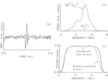
Application of the Wiener filter controlled by an estimated S/N

In the first example, measured noise from the stainless steel specimen is used along with a simulated flaw signal from a 67~m diameter sphere

to create a signal with a favorable S/N over the entire measurement system bandwidth. This example shows that the estimated S/N, [S/N)i, senses the favorable S/N and determines a filter shape which essentially passes everything within the measurement system bandwidth. Figure 2a shows the noise-corrupted time domain signal. Figure 2b shows the noise-free signal power spectrum, jRj2jAij2, and the average noise power spectrum, E[n2], for the stainless steel specimen (see Fig.

1).

Shown in the solid line in Fig. 2c is the filter shape determined by [S/N)i in combination with the cosine squared window. Shown in dashed line in the same figure is the

Q

2

=

O.OliR! 2max filter shape. As expected, the estimated S/N filter shape essentially passes everything within the measurement system bandwidth. For this case, that is when the S/N is favorable throughout the bandwidth, the q2

=

O.OljRj 2max filter approximates the estimated S/N filter quite well.

The second example uses measured noise from the aluminum specimen and a simulated flaw signal from a 200~m diameter sphere. This example

shows that the estimated S/N senses the noise dominance at low frequenc y and de termines a filter shape which goes to zero within the bandwidth at low frequency. Figure 3a shows the noise corrupted time domain signal. Figure 3b shows the noise-free signal power spectrum and the average noise power spectrum. Figure 3c shows both the filter shape determined by [S/N)i in combination with the cosine squared window and the q2

=

O.OljRj2max

0 . 0

~

~

~

o ~ ~

~ ~

(a) ~

~

~ o ~

2 .0 TIHE (~s)

o

o

8 16

FREQUENCY (MHz)

t

Estimated S/N Filte r

Desensitization Fi l ter

8 16

FREQUENCY (MHz) Fi g . 2 . Fi l te ring with a hi gh S/N t hrougho11 t the hRn~w irlth.

(b)

24

(c)

[image:7.505.76.432.368.632.2]

Q)

....

"'

(J

CI)

.D

_...

"'

...:1 0.. ~ (a)

L---~---0.0 2.0

TII-lE (vs)

l.O w :::> ...:1 < >

"'

w 1-< ...:1

....

""

0.0

o

Desensitization Filter Estimated s/N Filter

8 16

FREQUENCY (MHz)

.

.

24

--.

Q)

....

(b)

From

Desensitization Computer

"'

(J

"'

.D

_...

"'

o

8 16 24

FREQUENCY (MHz)

,....

Gl Filter

"'

(J

"'

.D

_...

[image:8.505.74.426.44.333.2]

<O

...

< ... Q)

"'

From ~- Estima ted

S/N Fi1ter

8 16

FREQUENCY (MHz)

Fig . 3. Filtering with a low S/N within the hanrlwidth.

24

filter shape. As expecterl, the filter shape determined via the e stimated S/N reflects the noise dominance by going to zero within the bandwidth at low frequency. The

Q

2

₌

O.OliRI 2max filter shape is insensitive to the noise and passes everything within the bandwidth including the noise dominated low frequencies. Figure 3d shows the computer generated real part of the scattering amplitude (Re(Ai)) along with the scattering amplitude estimates determined by multiplying the unfiltered scattering amplitude estimate by each of the filters shown in Fig . 3c. The scattering amplitude estimate determined with the

q2

=

O.OliRI2max fil ter shows the noise domi-nance at low frequency. On the other hand, the estimated S/N filter, which is sensitive to the noise dominance, forces the scattering amplitude estimate to zero at low frequency.

SUMMARY

The thrust of this paper has been to examine the Wiener filter scatter-ing amplitude estimation concept rather than evaluation of the Wiener filter as used in conjunction with a flaw characterization algorithm. The examination step i s a necessary step which has lead to 1) a procedure

The evaluation step will be the thrust of the next stage of this project. Evaluation of the optimality of any scattering amplitude estimate must be made relative to some criterion. Two points which have not been discussed influence this optimality criterion. First, scattering amplitude estimation is typically not a single step process. Frequently, filtering is followed by extrapolation. Extrapolation is based on ~ priori knowledge beyond that which is utilized by the Wiener filter. When scattering ampli-tude estimation is a two step process, it is the goal of the process, not the filtering step alone, to determine the optimal scattering amplitude estimate. Second, recall that flaw characterization is the motivation behind scattering amplitude estimation. The overall goal is to optimally characterize the flaw. An optimum scattering amplitude estimate is that estimate which will lead to optimal flaw characterization. Note that the maximum likelihood based Wiener filter scattering amplitude estimation technique associates optimality with the most probable scattering amplitude estimate. This optimality criterion may not be the most appropriate criter-ion since it does not take into account either of the points just discussed.

Finally, the significance of the S/N estimate as a function of fre-quency should be emphasized. Note that the scattering amplitude estimate itself gives no quantitative indication of the quality of the scattering amplitude estimate. It is knowledge of the filter shape (which is equiva-lent to knowledge of the S/N as a function of frequency) which is useful in establishing the quality of the scattering amplitude estimate.

ACKNOWLEDGEMENT

The Ames Laboratory is operated for the U.S. Department of Energy by Iowa State University under Contract No. W-7405-ENG-82. This work was supported by the Director of Energy Research, Office of Basic Energy Sciences.

REFERENCES

1. Y. Murakami, B. T. Khuri-Yakub, G. D. Kino, J. M. Richardson, and A. G. Evans, "An application of Wiener filtering to nondestructive evaluation", Appl. Phys. Lett. 33(8), (1978).

2. R. K. Elsley, J. M. Richardson, and R. C. Addison, "Optimum measurement of broadband ultrasonic data", in, 1980 Ultrasonics Symposium

Proceedings, IEEE, New York, (1980).

3. R. B. Thompson and T. A. Gray, "A model relating ultrasonic scattering measurements through liquid-solid interfaces to unbounded medium scattering amplitudes", J. Acoust. Soc. Am. 74(4), (1983). 4. D. O. Thompson and S. J. Wormley, "Long and intermediate wavelength