Remeshing techniques for r-adaptive and combined h/r-adaptive analysis with application to 2D/3D crack propagation

REMESHING TECHNIQUES FOR

R

-ADAPTIVE AND

COMBINED

H/R

-ADAPTIVE ANALYSIS WITH

APPLICATION TO 2D/3D CRACK PROPAGATION

H. Askes, L.J. Sluys†, and B.B.C. de Jong‡

Koiter Institute Delft / Delft University of Technology, Faculty of Civil Engineering and Geosciences, P.O. Box 5048, 2600 GA Delft, The Netherlands,

email: [email protected],

†_{[email protected],} ‡_{[email protected],}

URL:www.mechanics.citg.tudelft.nl

Key words: adaptivity, remeshing, ALE, crack propagation, failure analysis, localization

1 INTRODUCTION

Failure analyses of real-type engineering problems often require that mechanical pro-cesses on a much smaller scale are taken into account. For instance, a proper description of cracking phenomena is needed to account for a correct simulation of structural failure. Enhanced continuum material models such as the nonlocal damage model are suited to capture the crack propagation process in a physically realistic manner [1, 2]. With an en-hanced continuum material model the cracks are simulated as zones where strains localize, i.e. intense straining concentrates in the so-called localization zones. Numerical solution strategies, such as the finite element method, provide the tools to carry out the simula-tions. However, very fine meshes are needed to capture the localized strain fields correctly. The use of overall fine meshes leads to a highly inefficient computation, since then also the zones where no cracks occur are discretized with small elements. As a consequence, the computational costs in terms of CPU time and memory requirements rise dramatically, especially in three-dimensional analysis, which precludes a straighforward application of failure analysis with continuum models to engineering practice.

In order to balance the accuracy requirements and the efficiency requirements of nu-merical failure analysis adaptive techniques can be applied. The aim of using mesh-adaptive techniques is to optimize the spatial discretization such that the element size is small enough in the complete domain. The criterion with which the desired element size is computed is normally provided by the user, for instance by means of error as-sessment and a given error tolerance. Several adaptive techniques have been proposed

in the literature, including h-adaptivity, p-adaptivity and r-adaptivity [3, 4]. h-adaptive

schemes change the mesh connectivity constantly through the addition or deletion of el-ements. The enrichment of the polynomial interpolation space in certain regions, which

characterises p-adaptivity, requires special interface constructions between elements with

different interpolation polynomials. The relocation of nodes with invariant element

con-nectivity as occurs inr-adaptive schemes prohibits the addition or deletion of degrees of

freedom regardless an initially too coarse or too dense mesh. Whereash-adaptive schemes

and p-adaptive schemes are suitable for achieving a prescribed accuracy upon repeated

refinement, r-adaptive schemes can make an optimal use of a given mesh topology, so

that reasonable solutions can be obtained at minimal computational costs. Indeed, it has

been shown that the computational overhead of r-adaptive schemes can be made

neg-ligible. More specifically, the difference in computer costs of analyses with and without

r-adaptivity can be made as low as O(N) with N the number of elements [5–7]. In

con-trast, the continuous construction of a completely new mesh as it is done in h-adaptivity

can be a time-consuming task, especially in a three-dimensional analysis.

However, the applicability of r-adaptivity is limited since the number of degrees of

freedom and the element connectivity cannot be changed. For a more flexible formulation,

r-adaptivity and h-adaptivity can be combined. Indeed, the advantages of h-adaptivity

which can be used to optimize a given finite element configuration, h-adaptivity can be

applied to construct a new mesh wheneverr-adaptivity is not capable of further improving

the mesh. Therefore, a combined h/r-adaptive approach is more flexible than a fully r

-adaptive approach, so that the limitations ofr-adaptivity can be overcome. On the other

hand, a combined h/r-adaptive scheme can be more efficient than a fully h-adaptive

scheme, since at certain stages r-adaptive remeshing can be used instead of the more

expensive h-adaptive remeshing.

In this study we formulate r-adaptive and h/r-adaptive strategies for the analysis of

crack propagation. A heuristic error indicator is derived from an analysis of dispersive waves [7–10]. With this error indicator remeshing strategies are elaborated which allow for mesh refinement in the zones of interest, i.e. cracked zones and zones where cracking is about to occur. Two and three-dimensional examples show the performances and the limitations of each of the approaches.

2 NONLOCAL DAMAGE THEORY

An isotropic damage theory is used in which the stresses σ are related to the strainsε

as

σ = (1−ω)D ε (1)

in which ω is the scalar damage and D contains the elastic stiffness moduli. Damage

growth is determined via an equivalent strain ε_eq which is defined as [11]

εeq =

(k_ct−1)I₁ 2k_ct(1−2ν) +

1 2k_ct

(kct−1)2I12

(1−2ν)2 +

2k_ctJ₂

(1 +ν)2 (2)

where k_ct denotes the ratio of compressive strength over tensile strength (taken here as

kct = 10) while the strain invariants I1 and J2 are defined as

I1 =ε1+ε2+ε3 (3)

J2 = (ε1−ε2)2+ (ε2−ε3)2+ (ε3−ε1)2 (4)

withε₁,ε₂ andε₃the principal strains. A damage loading function is defined asf =ε_eq−κ

where the history parameter κ= max(ε_eq, κ₀) and the damage threshold κ₀ is a material

parameter. If f = 0 and ˙f = 0 then damage grows according to

ω = 1− 1

1 +b(ε_eq−κ₀) (5)

with b a parameter that sets the softening behaviour of the material.

The above model lacks a parameter that sets the width of the zone in which damage

on the applied element size. To overcome these deficiencies, a nonlocal formalism is taken in that the equivalent strain is averaged over a representative volume as [2]

εeq(x) =

V α(s)εeq(x+s) dV

V α(s) dV

(6)

In Eq. (6), the weighting function α_(s) sets the representative volume. It is normally

taken as a decaying non-negative function. Here, the error function is taken as α_(s) =

exp(−|s|/2l2_c) wherel_cis a length scale parameter that sets the size of the averaging volume

in Eq. (6). The nonlocal equivalent strain ε_eq replaces the local equivalent strain ε_eq in

the damage loading function and the damage evolution function (5). As a consequence,

the length scale l_c sets the size of the damaging zone, so that mathematically well-posed

differential equations result and mesh-objective results can be obtained [2, 12].

3 DETERMINATION OF THE DESIRED ELEMENT SIZES

While a nonlocal framework in the constitutive relations can guarantee mesh-objective solutions in the whole loading process, mesh-adaptivity is needed to make failure analyses available for engineering practice. Without adaptive techniques, computational analysis either becomes very inefficient (when a fine mesh is used in the whole domain) or inaccu-rate (when a coarse mesh is used in the whole domain). Adaptive procedures can generally be considered to consist of two stages. Firstly, the error of the numerical solution must be assessed, and secondly this information on the error must be translated into an im-proved mesh which is expected to meet the error tolerances. This section deals with error assessment, while the adaption of the finite element mesh is discussed in the next section.

Following the terminology of Huerta et al. [3], we distinguish between error estimators

on one hand and error indicators on the other. The former provide an estimation of

the true error, which can be derived from mathematical considerations, and are mostly expensive in terms of computer time. The latter do not approximate the magnitude of

the true error but only give an indication where the error is large and where it is small.

Normally, they can be determined directly from the state variables, which makes them cheap to compute [3]. In either case, the error quantity must be translated into a pointwise defined desired element size to serve as an input for the remeshing algorithm.

In an infinitely long one-dimensional medium, a harmonic perturbation of the

displace-ment field yields the phase velocitycas a function of the (assumedly uniform) strain state

ε0, see References [1,8,10,12] for details of the derivation. For the nonlocal damage model

applied in this study, the phase velocity is expressed as

c2

c2

e

= (1−ω₀)−ε₀ ∂ω

∂εeq

exp

−k2lc2

2

(7)

where c_e =

E/ρ is the one-dimensional tensile wave velocity, E is Young’s modulus, ρ

is the mass density, ω₀ is the uniform damage state that corresponds to ε₀ and k is the

wave number for which the phase velocity cis computed. In dynamic analyses, the wave

velocitycmust be real [1,8,9,13,14]. Equivalently, in static analyses c= 0 [9,12]. As such,

a critical wave number k_crit can be derived above which the right hand side in Eq. (7) is

positive. Next, a critical wave length λ_crit can be derived by using λ = 2π/k [1, 8, 13, 14]

as

λcrit =

√

2πl_c

lnb+ lnε₀+ ln(1 +b(ε₀−κ₀))

(8)

where Eq. (5) has been substituted. This critical wave length is the maximum wave length that can still propagate through the damaged zone [1,9]. It sets the width of the zone over which damage can grow [1, 9, 13, 14]. Thus, Eq. (8) relates the width of the localization

zone to the strain level. Note that the critical wave length λ_crit is directly proportional to

the internal length scale l_c.

Eq. (8) gives the critical wave length for a continuous medium, i.e. prior to finite

element discretisation. In a similar manner, an expression for the critical wave length in a

discretised medium can be found [9]. This latter expression relates the critical wave length not only to the strain level, but also to the applied element size. An upper bound on the deviation between approximate (numerical) critical wave length and the exact (continous) critical wave length then leads to an upper bound for the element size. For instance, for a gradient-dependent plastic material it has been derived that 12 linear finite elements are needed to capture the localization zone if a 10 % mismatch between discrete critical wave length and continuous critical wave length is accepted [9]. As such, dispersion analysis can be used to derive an error measure which in the terminology of Huerta et al. is denoted anerror indicator [3]. An advantage is that the error indicator only depends on the state variables and the discretisation measures, which are readily available. Thus, the error indicator is cheap to compute. On the other hand, when a different material model or different damage loading function is used, the behaviour of the error indicator changes.

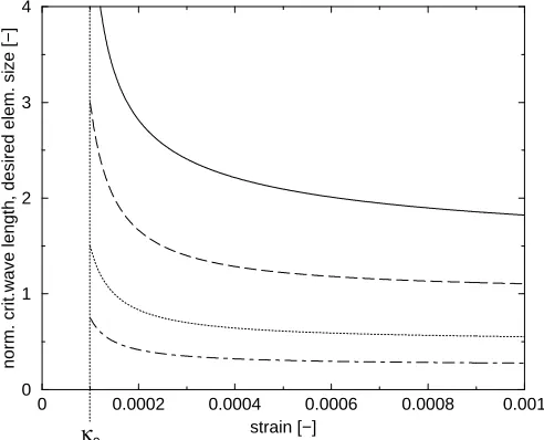
Combining the analytical considerations of dispersion analysis with the numerical ex-perimentation, we use the expression of the critical wave length Eq. (8) to determine an element size that is deemed suitable to capture the damage and strain fields adequately.

This element size will be denoted the desired element size in the sequel. Simple formulae

are postulated that relate the desired element size to the strain level, with the require-ment that the desired elerequire-ment size remains well below the critical wave length, so that it is guaranteed that a large enough number of elements is used inside the localization zone. For the elements in which damage takes place an expression that meets this requirement reads

desired element size = h₁−(h₁−h₂)ω (9)

where h₁ is the desired element size for ω = 0 or ε_eq =κ₀, and h₂ is the desired element

size for ω = 1. By setting values forh₁ and h₂, implicitly an error tolerance is provided.

0 0.0002 0.0004 0.0006 0.0008 0.001

strain [−] 0

1 2 3 4

norm. crit.wave length, desired elem. size [−]

κ0

Figure 1: Normalized critical wave length (solid) and normal-ized desired element size for h2/lc = 1 (dashed), h2/lc = 0.5 (dotted) andh2/lc = 0.25 (dot-dashed),h1/h2= 3 for all cases In Figure 1 the critical wave

length and the desired element size (both normalized with re-spect to the internal length scale

lc) are plotted as a function of

the strain level, for a range of

val-ues for h₁ and h₂. For the chosen

range of h₁ and h₂ the desired

el-ement sizes are smaller than the critical wave length.

While the above arguments give a desired element size for in-elastic zones, a sufficiently fine mesh is equally important in the elastic zones. Too large elements in the elastic regions can signifi-cantly delay or disturb the crack initiation and crack propagation processes [6, 15, 16]. Therefore, it should be ensured that element

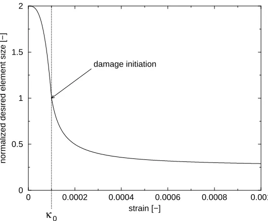
sizes are small enough in regions where cracking is about to occur. To this end, a de-sired size is also defined for elements that are still undamaged. Obviously, the dede-sired element size should be a continuous function of the strain level. Similar to Eq. (9) we define for the elastic regime

desired element size =h₀−(h₀−h₁)

_ε

eq

κ0

n

(10)

in which h₀ is the desired size for elements where no strains are present. The ratioε_eq/κ₀

a progressive decrease of the desired element size in the elastic regime [6].

0 0.0002 0.0004 0.0006 0.0008 0.001

strain [−] 0

0.5 1 1.5 2

normalized desired element size [

−

]

κ0

damage initiation

Figure 2: Desired element size normalized with respect to inter-nal length scale versus strain level – elastic and inelastic regime Note that for damage

initia-tion, i.e. ε_eq = κ₀ Eqns. (9) and

(10) yield the same desired ele-ment size. In Figure 2 the desired element size as a function of the strain level has been plotted for

h0/lc = 2, h1/lc = 1, h2/lc = 0.25

and n = 3. Around the stage of

damage initiation the desired el-ement size changes most rapidly, while for very small strains and very large strains the desired el-ement size does not change much. For very large strains, this means

that little additional refinement

is performed once a damage zone has been formed.

Special notice must be paid to the case that the strains go to in-finity. From Eq. (8) it can be seen

that then the critical wave length goes to zero, and so does the width of the zone where damage can grow. Thus, the nonlocal damage model applied here loses its regularising properties for infinite strains. As a consequence, infinitely small elements would be needed to capture this phenomenon correcly. However, the strain level at which this occurs is well beyond the range where the small strain assumption holds, and for the examples presented in this study the desired element size never becomes larger than the critical wave length.

4 REMESHING STRATEGY

The desired element sizes, determined in the previous section, are used as input in the

remeshing stage. Different remeshing strategies are formulated for r-adaptive remeshing

and for combined h/r-adaptive remeshing. For the r-adaptive framework an Arbitrary

Lagrangian-Eulerian [17–19] context is taken.

4.1 r-adaptive remeshing

In an r-adaptive context, nodes can be relocated so that element sizes can be adjusted

in the entire domain. However, no degrees of freedom can be added. The optimal mesh is therefore obtained by equidistributing the error quantity, that is, by requiring that the product of error and element size yields the same value for each element. Since for

equidistribution condition is written as [6, 7, 12, 21]

∂ ∂χ

1

hdes

∂x ∂χ

= 0 (11)

wherexare the spatial coordinates of the nodes, i.e. the unknowns that have to be solved

for, andχis a reference coordinate system associated with the mesh, i.e. each node has a

unique and invariant reference coordinate χ [17–19].

Eq. (11) can be repeated for each spatial coordinate. Thus, a system of differential

equations is found that is nonlinear sinceh_des=h_des(x). Boundary conditions are imposed

such that boundary nodes can only move along the boundary [19]. Directly applying a

Galerkin variational principle to Eq. (11) yields a system of algebraic equations as

A x=b (12)

wherexare the discretized unknowns, i.e. the spatial coordinates of each node,A is given

by

A=

V

ξ=x1,x2,x3 ∂HT

∂ξ

1

hdes

∂H

∂ξ dV (13)

and b contains the known components of A x that follow from the boundary conditions.

The matrixH contains the shape functions in the χ-coordinate system, that is,H should

be invariant and does not change after remeshing is carried out [6]. Eq. (12) will be referred

to as the elliptic equidistribution equation, since it ensues from the elliptic equation (11).

Since Eq. (11) is nonlinear, Eq. (12) must be solved iteratively. With multiple matrix inversions this form a major drawback, therefore it has been proposed to modify the right-hand-side of Eq. (11) as [6, 7, 12, 22]

∂ ∂χ

1

hdes

∂x ∂χ

= ∂x

∂τ (14)

where a pseudo-timeτ has been introduced that has no physical meaning but is only used

for computational convenience. Eq. (14) can be solved by means of relaxation. Discreti-sation yields [6, 7]

−A x+b=Q∂x

∂τ (15)

where A and b are the same as in Eq. (12) and with

Q=

V

HT_{HdV (16)}

Eq. (15) can be solved by means of a Forward Euler scheme, e.g. When matrix Q is

efficient compared to the solving of Eq. (12). Eq. (15) is denoted thepartial equidistribution equation, as it follows from the parabolic equation (14). It has been argued that taking

the pseudo-time step ∆τ < h2₂ leads to stable solutions with the Forward Euler scheme [6].

After the new nodal coordinates have been found, the stresses, strains and internal variables are transported to the new mesh using a Godunov algorithm [5, 15, 23, 24]. For elements with one integration point, the value of a state variable component after

remeshing ηnew _{is related to the value before remeshing η}old _via

ηnew _=ηold₊ 1

2Vel

Ns

s=1

Fs

ηold_−ηold adj

(1−sign(F_s)) (17)

where Vel _{is the element volume, N}

s is the number of sides of the element, ηadjold is the

value ofηold _{in the element adjacent to side} s_{, and the flux} F

s through side s is given by

Fs =

s

−nT_{∆xds (18)}

with n the normal to side s and ∆x the mesh incremental displacements, i.e. the mesh

displacements that follow from Eq. (12) or Eq. (15). Extenstion towards elements with multiple integration points is straightforward [5, 15, 23, 24]. Note that the computer costs

involved with Eq. (17) are O(N), which also holds for r-adaptive remeshing with the

parabolic equidistribution equation (15) [6, 10].

4.2 h/r-adaptive remeshing

One of the disadvantages of r-adaptive remeshing is that the number of degrees of

freedom remains fixed to the initial number. When this initial number is too low to capture

all the characteristics of the simulation properly, r-adaptivity will not provide accurate

solutions. Similarly, the element connectivity is invariant in r-adaptivity. If remeshing

leads to badly shaped elements, then the accuracy may drop. As an enhancement to the

fully r-adaptive approach, a combination of h-adaptivity and r-adaptivity is proposed.

Here, r-adaptivity is used as the default remeshing tool, while h-adaptivity is applied

whenever r-adaptivity is not suitable of further improvement of the mesh.

To assess the remeshing capacities ofr-adaptivity objectively, the concepts ofRefinement

Ratio and Aspect Ratio are introduced as

RR= current element size

desired element size (19)

and

AR = longest side of triangle

shortest height of triangle (20)

respectively. Obviously, values ofRRandARclose to one are optimal, while larger values

1. An r-adaptive step is performed

2. If the resulting mesh leads to too high values for AR or RR, then the r-adapted

mesh is discarded and h-adaptivity is carried out

Performing an r-adaptive step while it is unknown whether this will lead to an

accept-able discretisation seems a waste of computer time. However, since the computer costs

associated with r-adaptivity are as low as O(N) this is acceptable.

The remeshing strategy for combined h/r-adaptivity now splits into two strategies,

namely one for h-adaptivity and one for r-adaptivity. For h-adaptivity the computed

desired element sizes are used directly as input for the mesh generator. Thus, the quality

of the mesh generator determines the effectivity of h-adaptivity. After a new mesh has

been constructed, the state variables are projected from the old mesh onto the new mesh by means of the interpolation algorithm proposed by Ortiz and Quigley [25]. For each integration point in the new mesh the corresponding element in the old mesh must be found. Sophisticated search algorithms are needed to limit the computer time that is

necessary for this projection of the state variables, while a computational effort of O(N)

seems theoretically impossible.

For ther-adaptive steps in the combined approach the algorithm of Section 4.1 is taken

as the starting point. However, Eqns. (11) and (14) cannot be applied straightforwardly.

The reason is that the reference coordinates χ are fixed on the mesh and should be

in-variant during the analysis. However, when anh-adaptive step is performed, the reference

coordinates lose sense. It would be preferable to express Eqns. (11) and (14) in terms

of the current configuration, rather than terms of the reference or initial configuration.

Therefore, the derivatives with respect to χare rewritten into derivatives with respect to

the current spatial coordinates of the nodes using the chain rule [7, 10, 26]. For instance, Eq. (11) then becomes

∂ ∂xcur

1

hdes

∂x ∂xcur

∂xcur

∂χ

∂xcur

∂χ = 0 (21)

The ratio ∂x_cur/∂χ is non-zero and it is proportional to the current element size [10, 26].

Therefore, Eq. (21) can be elaborated as

∂ ∂xcur

RR_∂x∂x

cur

= 0 (22)

Eq. (22) only contains quantities associated with the current configuration. Thus,

gener-ality is preserved. The parabolic equidistribution equation (14) can be transformed in a similar manner.

5 EXAMPLES

Two examples are presented here. The first concerns with the remeshing capacities of

5.1 Dynamically loaded beam with eccentric notch

55

50 mm mm

140 mm

10 mm mm

37.5

v ^

20 mm

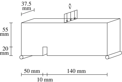
Figure 3: Beam with eccentric notch – problem state-ment

A three-dimensional dynamically loaded beam is studied. An eccentric notch is present, which drives the formation of a cracked zone that starts at the notch tip and propagates towards the top of the spec-imen. The geometry and loading conditions are given in Figure 3. The imposed velocity

increases linearly from ˆv = 0 mm/s at time

t= 0 s to ˆv = 2 mm/s at time t= 2·10−4

s, after which it remains constant. The

ma-terial parameters are taken as E = 31000

N/mm2_{, ν = 0.2, ρ = 2.4·10}−9 _Ns/mm4_,

lc = 2 mm, κ0 = 3.5·10−4 and b = 20000.

Two meshes have been used, one consisting of 9393 linear tetrahedrons and one

consist-ing of 1503 linear tetrahedrons. Both meshes are non-uniform in the sense that the mesh density is larger in the area around the notch. The finer mesh is only used in a

non-adaptive analysis. With the coarser mesh a non-non-adaptive analysis as well as r-adaptive

analyses have been carried out. For ther-adaptive analyses the valuesh₀/h₁ andh₀/h₂ are

taken as 2 and 5, respectively1. Equidistribution is carried out with the elliptic equation

as well as with the parabolic equation. For the parabolic equation the pseudo-time step

∆τ = 0.05.

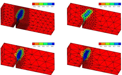
Figure 4 shows the damage contours for the four analyses at time t = 10−3 s. The

fine non-adaptive mesh gives a damage pattern where the crack propagates from the notch upwards with a specific inclination angle. When the coarse non-adaptive mesh is considered, it can be seen that the inclination angle does not correspond to that of the fine non-adaptive mesh. Also, the damage values inside the cracked zone are not predicted correctly. On the other hand, when the same coarse mesh is used as the initial mesh in an

r-adaptive context, much better results are obtained. For the adaptive analyses, both the

inclination angle and the maximum damage values inside the cracked zone are in good agreement with the fine non-adaptive mesh. Thus, by adjusting the nodal coordinates, the accuracy of a fine mesh can be attained by a much coarser mesh.

A next observation is that the performance of the two equidistribution equations is similar. Although minor differences are present, both capture the inclination angle and the peak damage values properly.

However, as can be seen from the adaptive meshes in Figure 4, not much further 1_{Eq. (11) can be multiplied with h}

0.1 0.3 0.5 0.7 0.9 0.1 0.3 0.5 0.7 0.9

0.1 0.3 0.5 0.7 0.9 0.1 0.3 0.5 0.7 0.9

Figure 4: Beam with eccentric notch – damage contours for fine non-adaptive mesh (upper left), coarse non-adaptive mesh (upper right),r-adaptive mesh with elliptic equidistribution (lower left) andr-adaptive mesh with parabolic equidistribution (lower right)

improvement of the discretisation is possible. The number of available elements precludes that newly appearing cracks could be described adequately. Moreover, the aspect ratios of the elements above the cracked zone have become very large, which can be a source of inaccuracy. When further mesh refinement is desired, a new mesh has to be constructed.

5.2 Single-edge-notched beam

F F

20

80 mm 20 mm

9 20

y x

5 180 mm

180 mm

Figure 5: Single-edge-notched beam – problem statement In the second example we

study a single-edge-notched beam. The beam is subjected to a static four-point loading, which results in the forma-tion of a curved crack that starts at the notch tip. Fur-thermore, a secondary, bend-ing crack may appear oppo-site of the centremost sup-port. The material

N/mm2_{,ν = 0.2,l}

c = 1 mm, κ0 = 1.2·10−4 and b= 20000. The load platens are modelled

with a 10 times higher Young’s modulus.

0.1 0.3 0.5 0.7 0.9

0.1 0.3 0.5 0.7 0.9

0.1 0.3 0.5 0.7 0.9

0.1 0.3 0.5 0.7 0.9

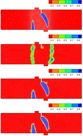
Figure 6: Single-edge-notched beam – damage contours for CMSD = 0.04 mm, fine non-adaptive mesh, coarse non-adaptive mesh, h -adaptive mesh andh/r-adaptive mesh (top to bottom)

An indirect displacement control procedure is used to apply the load [27], whereby the crack mouth sliding dis-placement (CMSD) is used as the control parameter. The CMSD is defined as the difference in vertical dis-placement between the two top nodes at either side of the notch. Two non-adaptive meshes have been used, one consisting of 11419 elements and one of 1761 elements. The finer mesh is selected such that is has an element

size of 1.5 mm in the

cen-tral region. Furthermore, a

combined h/r-adaptive

anal-ysis has also been carried out whereby the coarse non-adaptive mesh is taken as the initial mesh. The desired el-ement size is computed with

h0 = 7 mm, h1 = 3 mm and

h2 = 1 mm. An h-adaptive

step is carried out whenever the refinement ratio of an ele-ment exceeds the value 1.5 or when the aspect ratio exceeds the value 4. As a comparison,

also anh-adaptive analysis is

carried out where remeshing

is performed whenRR >1.5.

Figure 6 shows the damage contours for the four analyses for CMSD = 0.04 mm. A first

x (y=x-160)

d

a

m

a

g

e

[-]

200 210 220 230 240

0 0.2 0.4 0.6 0.8 1

x (y=x-160)

d

a

m

a

g

e

[-]

140 150 160 170 180

0 0.2 0.4 0.6 0.8 1

Figure 7: Single-edge-notched beam – damage profiles for CMSD = 0.04 mm along the linesy=x−160 (left) andy= 20 (right), fine Lagrangian analysis (solid),h-adaptive analysis (dotted) and h/r-adaptive analysis (dashed)

literature [11], the coarser mesh predicts a completely different failure mode. Due to the coarse discretisation at the notch tip, the stress singularity cannot be captured properly and the dominant, curved crack cannot develop. Alternatively, two bending cracks appear at either side of the beam. Obviously, this is due to the incapabilities of the mesh to describe the correct failure pattern.

The situation is different for the two adaptive analyses. For these two cases, the crack pattern is predicted correctly, while also the damage values inside the cracked zone corre-spond well with those of the fine non-adaptive mesh. Figure 7 offers a closer inspection of

the crack patterns, namely the damage profiles along the linesy=x−160 andy= 20 for

the fine non-adaptive mesh and the two adaptive meshes. Although both adaptive meshes overestimate the crack width somewhat, the basic trends are captured reasonably well.

Figure 8 shows the number of elements during the analysis for the two adaptive

compu-tations. Horizontal line segments denote that no remeshing is performed (h-adaptive test)

or thatr-adaptive remeshing is carried out (h/r-adaptive test). The number ofh-adaptive

remeshings is 69 in the h-adaptive test and 58 in the h/r-adaptive test. From Figure 8

it can be seen that in the middle stages of the computation the number of h-remeshings

is approximately the same for both tests. This corresponds to the stage where the cracks

propagate relatively fast. Then, r-adaptivity is less suited for remeshing purposes. In the

final stages of the computation, when little additional cracking takes place, r-adaptivity

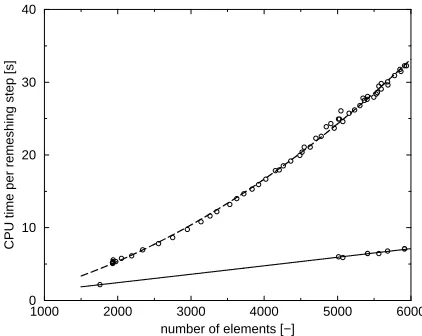
is better suited to optimize the mesh. In Figure 9 the CPU time per remeshing step is

plotted as a function of the number of elements forr-adaptive steps andh-adaptive steps

in the combinedh/r-adaptive analysis. A least squares approximation has been used to fit

a parabolic curve through the data. It can be seen that for theh-adaptive steps the CPU

0 0.2 0.4 0.6 0.8 1 time [s]

0 2000 4000 6000 8000

number of elements [

−

]

Figure 8: Single-edge-notched beam – number of elements during the analysis, h-adaptive mesh (dashed) andh/r-adaptive mesh (solid)

1000 2000 3000 4000 5000 6000 number of elements [−]

0 10 20 30 40

CPU time per remeshing step [s]

Figure 9: Single-edge-notched beam – CPU time per remeshing step versus number of elements in the combinedh/r-adaptive test,h-adaptive steps (dashed) andr-adaptive steps (solid)

hand, for the r-adaptive steps the CPU time is virtually a linear function of the number

of elements. Figure 9 confirms the O(N) computer costs of r-adaptivity as compared to

the higher costs involved with h-adaptivity.

6 CONCLUSIONS

Remeshing strategies are formulated and tested for the analysis of crack propagation. The nonlocal damage model is used to simulate the softening material behaviour. Based on the dispersive properties of the material, heuristic formulae are proposed to compute the desired element size as a function of the strain level. The desired element size is used as

input for r-adaptive remeshing and for a combination of r-adaptivity with h-adaptivity.

r-adaptivity is very cheap, while h-adaptivity is more flexible. Examples are presented

which show that r-adaptivity is able to optimize a given mesh topology. The accuracy

of a fine non-adaptive mesh can be approximated by a simple adjustment of the nodal

coordinates. However, the applicability of r-adaptivity is limited. The combined h/r

-adaptive approach is more flexible than a fullyr-adaptive approach in the sense that the

number of elements can be changed during the analysis. On the other hand, the combined

h/r-adaptive approach reduces the number of h-remeshings needed, so that computer

costs are limited.

ACKNOWLEDGEMENTS

REFERENCES

[1] L.J. Sluys, Wave propagation, localisation and dispersion in softening solids,

Disser-tation, Delft University of Technology, 1992.

[2] G. Pijaudier-Cabot and Z.P. Baˇzant, ‘Nonlocal damage theory’, ASCE Journal of

Engineering Mechanics, 113, 1512–1533 (1987).

[3] A. Huerta, A. Rodr´ıguez-Ferran, P. D´ıez, and J. Sarrate, ‘Adaptive finite element

strategies based on error assessment’, International Journal for Numerical Methods

in Engineering,46, 1803–1818 (1999).

[4] O.C. Zienkiewicz and J.Z. Zhu, ‘Adaptivity and mesh generation’, International

Journal for Numerical Methods in Engineering, 32, 783–810 (1991).

[5] A. Rodr´ıguez-Ferran, F. Casadei, and A. Huerta, ‘ALE stress update for transient and

quasistatic processes’, International Journal for Numerical Methods in Engineering,

43, 241–262 (1998).

[6] H. Askes and L.J. Sluys, ‘Remeshing strategies for adaptive ALE analysis of strain

localisation’, European Journal of Mechanics A/Solids, accepted for publication.

[7] H. Askes, Advanced spatial discretisation strategies for localised failure — mesh

adap-tivity and meshless methods, Dissertation, Delft University of Technology, 2000.

[8] A. Huerta and G. Pijaudier-Cabot, ‘Discretization influence on the regularization

by two localization limiters’, ASCE Journal Engineering Mechanics,120, 1198–1218

(1994).

[9] L.J. Sluys, M. Cauvern, and R. de Borst, ‘Discretization influence in strain-softening

problems’, Engineering Computations,12, 209–228 (1995).

[10] H. Askes and L.J. Sluys, ‘An alternating r-adaptive and h-adaptive strategy with

application to localized failure’, Mechanics of Cohesive-Frictional Materials,

submit-ted.

[11] R.H.J. Peerlings, R. de Borst, W.A.M. Brekelmans, and M.G.D. Geers,

‘Gradient-enhanced damage modelling of concrete fracture’, Mechanics of Cohesive-Frictional

Materials, 3, 323–342 (1998).

[12] L. Bod´e, Strat´egies num´eriques pour la pr´evision de la ruine des structures du g´enie

civil, Dissertation, E.N.S. de Cachan / CNRS / Universit´e Paris 6, 1994.

[13] R.H.J. Peerlings, Enhanced damage modelling for fracture and fatigue, Dissertation,

[14] R.H.J. Peerlings, R. de Borst, W.A.M. Brekelmans, J.H.P. de Vree, and I. Spee, ‘Some

observations on localisation in non-local and gradient damage models’, European

Journal of Mechanics, A/Solids, 15, 937–953 (1996).

[15] H. Askes, A. Rodr´ıguez-Ferran, and A. Huerta, ‘Adaptive analysis of yield line

patterns in plates with the arbitrary Lagrangian-Eulerian method’, Computers and

Structures,70, 257–271 (1999).

[16] H. Askes and L.J. Sluys, ‘Adaptive ALE analyses of crack propagation with a

con-tinuum material model’, in W. Wunderlich, editor,European Conference on

Compu-tational Mechanics — Solids, Structures and Coupled Problems in engineering. TU

M˝unchen, 1999.

[17] J. Don´ea, ‘Arbitrary Lagrangian-Eulerian finite element methods’, in T. Belytschko

and T.J.R. Hughes, editors, Computational methods for transient analysis,

chap-ter 10, pages 474–516. Elsevier, 1983.

[18] T.J.R. Hughes, W.K. Liu, and T.K. Zimmermann, ‘Lagrangian-Eulerian finite

el-ement formulation for incompressible viscous flows’, Computer Methods in Applied

Mechanics and Engineering, 29, 329–349 (1981).

[19] A. Huerta and F. Casadei, ‘New ALE applications in non-linear fast-transient solid

dynamics’, Engineering Computations, 11, 317–345 (1994).

[20] P. D´ıez and A. Huerta, ‘A unified approach to remeshing strategies for finite element

h-adaptivity’, Computer Methods in Applied Mechanics and Engineering,176, 215–

229 (1999).

[21] G. Pijaudier-Cabot, L. Bod´e, and A. Huerta, ‘Arbitrary Lagrangian-Eulerian finite

element analysis of strain localization in transient problems’, International Journal

for Numerical Methods in Engineering, 38, 4171–4191 (1995).

[22] L. Bod´e, G. Pijaudier-Cabot, and A. Huerta, ‘ALE finite element analysis of strain

localisation – consistent computational strategy and remeshing issues’, in D.R.J.

Owen, E. O˜nate, and E. Hinton, editors, Computational Plasticity IV, pages 587–

598. Pineridge Press, Swansea, UK, 1995.

[23] A. Huerta, F. Casadei, and J. Don´ea, ‘ALE stress update in transient plasticity

prob-lems’, in D.R.J. Owen, E. O˜nate, and E. Hinton, editors, Computational Plasticity

IV, pages 1865–1876. Pineridge Press, Swansea, UK, 1995.

[24] H. Askes, L. Bod´e, and L.J. Sluys, ‘ALE analyses of localization in wave propagation

[25] M. Ortiz and J.J. Quigley, ‘Adaptive mesh refinement in strain localization problems’,

Computer Methods in Applied Mechanics and Engineering,90, 781–804 (1991).

[26] H. Askes and A. Rodr´ıguez-Ferran, ‘A combinedrh-adaptive scheme based on domain

subdivision – Formulation and linear examples’, International Journal for Numerical

Methods in Engineering, submitted.

[27] R. de Borst, ‘Computation of post-bifurcation and post-failure behavior of