This is a repository copy of
Neural networks in geophysical applications
.
White Rose Research Online URL for this paper:
http://eprints.whiterose.ac.uk/325/
Article:
Van der Baan, M. and Jutten, C. (2000) Neural networks in geophysical applications.
Geophysics, 65 (4). pp. 1032-1047. ISSN 0016-8033
https://doi.org/10.1190/1.1444797
eprints@whiterose.ac.uk
https://eprints.whiterose.ac.uk/
Reuse
See Attached
Takedown
If you consider content in White Rose Research Online to be in breach of UK law, please notify us by
GEOPHYSICS, VOL. 65, NO. 4 (JULY-AUGUST 2000); P. 1032–1047, 7 FIGS., 1 TABLE.
Neural networks in geophysical applications
Mirko van der Baan
∗and Christian Jutten
‡ABSTRACT
Neural networks are increasingly popular in geo-physics. Because they are universal approximators, these tools can approximate any continuous function with an arbitrary precision. Hence, they may yield important contributions to finding solutions to a variety of geo-physical applications.
However, knowledge of many methods and tech-niques recently developed to increase the performance and to facilitate the use of neural networks does not seem to be widespread in the geophysical community. There-fore, the power of these tools has not yet been explored to their full extent. In this paper, techniques are described for faster training, better overall performance, i.e., gen-eralization, and the automatic estimation of network size and architecture.
INTRODUCTION
Neural networks have gained in popularity in geophysics this last decade. They have been applied successfully to a va-riety of problems. In the geophysical domain, neural networks have been used for waveform recognition and first-break pick-ing (Murat and Rudman, 1992; McCormack et al., 1993); for electromagnetic (Poulton et al., 1992), magnetotelluric (Zhang and Paulson, 1997), and seismic inversion purposes (R ¨oth and Tarantola, 1994; Langer et al., 1996; Calder ´on–Mac´ıas et al., 1998); for shear-wave splitting (Dai and MacBeth, 1994), well-log analysis (Huang et al., 1996), trace editing (McCormack et al., 1993), seismic deconvolution (Wang and Mendal, 1992; Calder ´on–Mac´ıas et al., 1997), and event classification (Dowla et al., 1990; Romeo, 1994); and for many other problems.
Nevertheless, most of these applications do not use more re-cently developed techniques which facilitate their use. Hence, expressions such as “designing and training a network is still more an art than a science” are not rare. The objective of this paper is to provide a short introduction to these new
Manuscript received by the Editor January 20, 1999; revised manuscript received February 3, 2000.
∗Formerly Universit ´e Joseph Fourier, Laboratoire de G ´eophysique Interne et Tectonophysique, BP 53, 38041 Grenoble Cedex, France; currently
University of Leeds, School of Earth Sciences, Leeds LS2 9JT, UK. E-mail: mvdbaan@earth.leeds.ac.uk.
‡Laboratoire des Images et des Signaux, Institut National Polytechnique, 46 av. F ´elix Viallet, 38031 Grenoble Cedex, France. E-mail: chris@lis-viallet.inpg.fr.
c
2000 Society of Exploration Geophysicists. All rights reserved.
techniques. For complete information covering the whole do-main of neural networks types, refer to excellent reviews by Lippmann (1987), Hush and Horne (1993), H ´erault and Jutten (1994), and Chentouf (1997).
The statement that “designing and training a network is still more an art than a science” is mainly attributable to sev-eral well-known difficulties related to neural networks. Among these, the problem of determining the optimal network config-uration (i.e., its structure), the optimal weight distribution of a specific network, and the guarantee of a good overall per-formance (i.e., good generalization) are most eminent. In this paper, techniques are described to tackle most of these well-known difficulties.
Many types of neural networks exist. Some of these have already been applied to geophysical problems. However, we limit this tutorial to static, feedforward networks. Static im-plies that the weights, once determined, remain fixed and do not evolve with time; feedforward indicates that the output is not feedback, i.e., refed, to the network. Thus, this type of network does not iterate to a final solution but directly trans-lates the input signals to an output independent of previous input.
Moreover, only supervised neural networks are consi-dered—in particular, those suited for classification problems. Nevertheless, the same types of neural networks can also be used for function approximation and inversion problems (Poulton et al., 1992; R ¨oth and Tarantola, 1994). Super-vised classification mainly consists of three different stages (Richards, 1993): selection, learning or training, and classifica-tion. In the first stage, the number and nature of the different classes are defined and representative examples for each class are selected. In the learning phase, the characteristics of each individual class must be extracted from the training examples. Finally, all data can be classified using these characteristics.
Nevertheless, many other interesting networks exist—un-fortunately, beyond the scope of this paper. These include the self-organizing map of Kohonen (1989), the adaptive resonance theory of Carpenter and Grossberg (1987), and the Hopfield network (Hopfield, 1984) and other recurrent
networks. See Lippmann (1987) and Hush and Horne (1993) for a partial taxonomy.
This paper starts with a short introduction to two types of static, feedforward neural networks and explains their general way of working. It then proceeds with a description of new tech-niques to increase performance and facilitate their use. Next, a general strategy is described to tackle geophysical problems. Finally, some of these techniques are illustrated on a real data example—namely, the detection and extraction of reflections, ground roll, and other types of noise in a very noisy common-shot gather of a deep seismic reflection experiment.
NEURAL NETWORKS: STRUCTURE AND BEHAVIOR
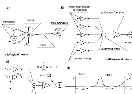
The mathematical perceptron was conceived some 55 years ago by McCulloch and Pitts (1943) to mimic the behavior of a biological neuron (Figure 1a). The biological neuron is mainly composed of three parts: the dendrites, the soma, and the axon. A neuron receives an input signal from other neurons con-nected to its dendrites by synapses. These input signals are attenuated with an increasing distance from the synapses to the soma. The soma integrates its received input (over time and space) and thereafter activates an output depending on the total input. The output signal is transmitted by the axon and distributed to other neurons by the synapses located at the tree structure at the end of the axon (H ´erault and Jutten, 1994).
FIG.1. The biological and the mathematical neuron. The mathematical neuron (b) mimics the behavior of the biological neuron
(a). The weighted sum of the inputs is rescaled by an activation function (c), of which several examples are shown in (d). Adapted from Lippmann (1987), H ´erault and Jutten (1994), and Romeo (1994).
The mathematical neuron proceeds in a similar but simpler way (Figure 1b) as integration takes place only over space. The weighted sum of its inputs is fed to a nonlinear transfer function (i.e., the activation function) to rescale the sum (Figure 1c). A constant biasθis applied to shift the position of the activation function independent of the signal input. Several examples of such activation functions are displayed in Figure 1d.
Historically, the Heaviside or hard-limiting function was used. However, this particular activation function gives only a binary output (i.e., 1 or 0, meaning yes or no). Moreover, the optimum weights were very difficult to estimate since this particular function is not continuously differentiable. Thus, e.g., first-order perturbation theory cannot be used. Today, the sigmoid is mostly used. This is a continuously differentiable, monotonically increasing function that can best be described as a smooth step function (see Figure 1d). It is expressed by
fs(α)=(1+e−α)−1.
[image:3.666.81.537.365.690.2]To gain some insight in the working of static feedforward networks and their ability to deal with classification prob-lems, two such networks will be considered: one composed of a single neuron and a second with a single layer of hidden neurons. Both networks will use a hard-limiting function for simplicity.
classes are separated by an (n−1)-dimensional hyperplane for ann-dimensional input.
More complex distributions can be handled if a hidden layer of neurons is added. Such layers lie between the input and out-put layers, connecting them indirectly. However, the general way of working does not change at all, as shown in Figures 3a and 3b. Again, each neuron in the hidden layer divides the input space in two half-spaces. Finally, the last neuron com-bines these to form a closed shape or subspace. With the ad-dition of a second hidden layer, quite complex shapes can be formed (Romeo, 1994). See also Figure 14 in Lippmann (1987).
Using a sigmoidal instead of a hard-limiting function does not change the general picture. The transitions between classes are smoothed. On the other hand, the use of a Gaussian activa-tion funcactiva-tion implicates major changes, since it has a localized response. Hence, the sample space is divided in two parts. The part close to the center of the Gaussian with large outputs is enveloped by the subspace at its tails showing small output
FIG.2. (a) Single perceptron layer and (b) associated decision boundary. Adapted from Romeo (1994).
FIG.3. (a) Single hidden perceptron layer and (b) associated decision boundary. Adapted from Romeo (1994).
values. Thus, only a single neuron with a Gaussian activation function and constant variance is needed to describe the gray class in Figure 3 instead of the depicted three neurons with hard-limiting or sigmoidal activation functions. Moreover, the Gaussian will place a perfect circle around the class in the mid-dle (if a common variance is used for all input parameters).
exact number of neurons needed since these are asymptotic re-sults. Moreover, applications exist where neural networks with two hidden layers produce similar results as a single hidden layer neural networks with a strongly reduced number of links and, therefore, a less complicated weight optimization prob-lem, i.e., making training much easier (Chentouf, 1997).
Two types of activation functions are used in Figure 1d. The hard-limiter and the sigmoid are monotonically increas-ing functions, whereas the Gaussian has a localized activation. Both types are commonly used in neural networks applications. In general, neural networks with monotonically increasing ac-tivation functions are called multilayer perceptrons (MLP) and neural networks with localized activation functions are called radial basis functions (RBF) (Table 1).
Hence, MLP networks with one output perceptron and a single hidden layer are described by
fMLP(x)=σ
nh1
k=1
wkσw(k)·x−θ(k)−θ
(1)
withσ(.) the sigmoidal activation function,xthe input,wkthe weight of linkkto the output node,nh1the number of nodes
in the hidden layer,w(k) the weights of all links to nodek in
the hidden layer, andθthe biases. Boldface symbols indicate vectors. Equation (1) can be extended easily to contain several output nodes and more hidden layers.
Likewise, RBF networks with a single hidden layer and one output perceptron are described by
fRBF(x)=σ
nh1
k=1
wkK
sk x−c(k)
−θ
(2)
with K(.) the localized activation function,. a (distance) norm,c(k)the center of the localized activation function in
hid-den nodek, andskits associated width (spread).
It is important to be aware of the total number (ntot) of
inter-nal variables determining the behavior of the neural networks structure used, as we show hereafter. Fortunately, this number is easy to calculate from equations. (1) and ( 2). For MLP net-works it is composed of the number of links plus the number of perceptrons to incorporate the number of biases. Ifnidenotes the number of input variables,nhithe number of perceptrons in theith hidden layer, andnothe number of output perceptrons, thenntotis given by
ntot=(ni+1)∗nh1+(nh1+1)∗no (3)
for an MLP with a single hidden layer and
ntot=(ni+1)∗nh1+(nh1+1)∗nh2+(nh2+1)∗no (4)
for an MLP with two hidden layers. The number of internal variables is exactly equal for isotropic RBF networks since each Gaussian is described byni+1 variables for its position and variance, i.e., width. Moreover, in this paper only RBF
net-Table 1. Abbreviations.
MLP Multilayer Perceptrons
NCU Noncontributing Units
OBD Optimal Brain Damage
OBS Optimal Brain Surgeon
PCA Principal Component Analysis
RBF Radial Basic Functions
SCG Scaled Conjugate Gradient
works with a single hidden layer are considered. In addition, only RBF neurons in the hidden layer have Gaussian activa-tion funcactiva-tions. The output neurons have sigmoids as activaactiva-tion functions. Hence,ntotis also given by equation (3).
As we will see, the rationtot/mdetermines if an adequate
network optimization can be hoped for, wheremdefines the number of training samples.
NETWORK OPTIMIZATION
Known problems
The two most important steps in applying neural networks to recognition problems are the selection and learning stages, since these directly influence the overall performance and thus the results obtained. Three reasons can cause a bad perfor-mance (Romeo, 1994): an inadequate network configuration, the training algorithm being trapped in a local minimum, or an unsuitable learning set.
Let us start with the network configuration. As shown in Figures 2 and 3, the network configuration should allow for an adequate description of the underlying statistical distribution of the spread in the data. Since the number of input and out-put neurons is fixed in many applications, our main concern is with the number of hidden layers and the number of neurons therein.
No rules exist for determining the exact number of neurons in a hidden layer. However, Huang and Huang (1991) show that the upper bound of number of neurons needed to reproduce exactly the desired outputs of the training samples is on the order ofm, the number of training samples. Thus, the number of neurons in the hidden layer should never exceed the num-ber of training samples. Moreover, to keep the training prob-lem overconstrained, the number of training samples should always be larger than the number of internal weights. In prac-tice,m≈10ntotis considered a good choice. Hence, the number
of neurons should be limited; otherwise, the danger exists that the training set is simply memorized by the network (overfit-ting). Classically, the best configuration is found by trial and error, starting with a small number of nodes.
A second reason why the network may not obtain the desired results is that it may become trapped in a local minimum. The misfit function is very often extremely complex (Hush et al., 1992). Thus, the network can easily be trapped in a local min-imum instead of attaining the sought-for global one. In that case even the training set cannot be fit properly.
Remedies are simple. Either several minimization attempts must be done, each time using a different (random or nonran-dom) initialization of the weights, or other inversion algorithms must be considered, such as global search.
Finally, problems can occur with the selected training set. The two most frequent problems are overtraining and a bad, i.e., unrepresentative, learning set. In the latter case, either too many bad patterns are selected (i.e., patterns attributed to the wrong class) or the training set does not allow for a good generalization. For instance, the sample space may be incomplete, i.e., samples needed for an adequate training of the network are simply missing.
[image:5.666.56.297.656.729.2]is often split into a training and a validation set. Weights are optimized using the training set. However, crossvalidation with the second set ensures an overall good performance.
In the following subsections, all of these problems are con-sidered in more detail, and several techniques are described to facilitate the use of neural networks and to enhance their performance.
Network training/weight estimation: An optimization problem
If a network configuration has been chosen, an optimal weight distribution must be estimated. This is an inversion or optimization problem. The most common procedure is a so-called localized inversion approach. In such an approach, we first assume that the outputycan be calculated from the input
xusing some kind of functionf, i.e.,y=f(x). Output may be contaminated by noise, which is assumed to be uncorrelated to the data and to have zero mean. Next, we assume that the function can be linearized around some initial estimatex0 of the input vectorxusing a first-order Taylor expansion, i.e.,
y=f(x0)+∂f(x0)
∂x x. (5)
If we write y0=f(x0), y=y−y0, and A(x)=∂f/∂x,
equa-tion (5) can also be formulated as
y=A(x)x, (6)
where the JacobianA(x)= ∇
xfcontains the first partial deriva-tives with respect tox. To draw an analogy with a better known inversion problem, in a tomography applicationywould con-tain the observed traveltimes,xthe desired slowness model, andAi jthe path lengths of rayiin cellj.
However, there exists a fundamental difference with a to-mography problem. In an neural networks application, both the outputyand the inputxare known, sincey(i)represents
the desired output for training samplex(i). Hence, the problem
is not the construction of a modelxexplaining the observations, but the construction of the approximation functionf. Since this function is described by its internal variables, it is another linear system that must be solved, namely,
y=A(w)w, (7)
where the JacobianA(w)= ∇
wfcontains the first partial deriva-tives with respect to the internal variables w. The vector w
contains the biases and weights for MLP networks and the weights, variances, and centers for RBF networks. For the ex-act expression ofA(w), we refer to Hush and Horne (1993)
and H ´erault and Jutten (1994). Nevertheless, all expressions can be calculated analytically. Moreover, both the sigmoid and the Gaussian are continuously differentiable, which is the ulti-mate reason for their use. Thus, no first-order perturbation the-ory must be applied to obtain estimates of the desired partial derivatives, implying a significant gain in computation time for large neural networks.
In general, the optimization problem will be ill posed since
A(w)suffers from rank deficiency, i.e., rank (A(w))≤n tot. Thus,
system (7) is underdetermined. However, at the same time, any well-formulated inversion problem will be overconstrained becausem≫ntot, yielding that there are more training samples
than internal variables.
Since system (7) is ill posed, a null space will exist. Hence, the internal variables cannot be determined uniquely. If, in addition,ntot≫mthen the danger of overtraining, i.e.,
mem-orization, increases considerably, resulting in suboptimal per-formance. Two reasons causeAto be rank deficient. First, the sample space may be incomplete, i.e., some samples needed for an accurate optimization are simply missing and some training samples may be erroneously attributed to a wrong class. Sec-ond, noise contamination will prevent a perfect fit of both pro-vided and nonpropro-vided data. For example, in a tomographic problem, rank deficiency will already occur if no visited cells are present, making a correct estimate of the true velocities in these cells impossible.
To give an idea of the number of training samples required, the theoretical study of Baum and Haussler (1989) shows that for a desired accuracy level of (1−ǫ), at leastntot/ǫexamples
must be provided, i.e.,m≥ntot/ǫ. Thus, to classify 90% of the
data correctly, at least 10 times more samples must be provided than internal variables are present, i.e.,m≥10ntot.
How can we solve equation (7)? A possible method of esti-mating the optimalwis by minimizing the sum of the squared differences between the desired and the actual output of the network. This leads to the least-mean-squares solution, i.e., the weights are determined by solving the normal equations
w=(AtA)−1Aty, (8)
where the superscript (w) is dropped for clarity.
This method, however, has the well-known disadvantage that singularities in AtA cause the divergence of the Euclidean norm|w|of the weights, since this norm is inversely propor-tional to the smallest singular value ofA. Moreover, ifAis rank deficient, then this singular value will be zero or at least effec-tively zero because of a finite machine precision. The squared norm|w|2is also often called the variance of the solution.
To prevent divergence of the solution variance, very often a constrained version of equation (8) is constructed using a positive damping variableβ. This method is also known as Levenberg–Marquardt or Tikhonov regularization, i.e., sys-tem (8) is replaced by
w=(AtA+βI)−1Aty, (9)
withIthe identity matrix (Lines and Treitel, 1984; Van der Sluis and Van der Vorst, 1987).
The matrixAtA+βIis not rank deficient in contrast toAtA. Hence, the solution variance does not diverge but remains con-strained. Nevertheless, the method comes at an expense: the solution will be biased because of the regularization parame-terβ. Therefore, it does not provide the optimal solution in a least-mean-squares sense. The exact value ofβmust be cho-sen judiciously to optimize the trade-off between variance and bias (see Van der Sluis and Van der Vorst, 1987; Geman et al., 1992).
More complex regularization can be used on bothwand
Just as in tomography problems, equations (8) and (9) are rarely solved directly. More often an iterative approach is ap-plied. The best known method in neural networks applications is the gradient back-propagation method of Rumelhart et al. (1986) with or without a momentum term, i.e., a term analogous to the function of the regularization factorβ. It is a so-called first-order optimization method which approximates (AtA)−1
in equations (8) and (9) byαIwithβ=0.
This method is basically a steepest descent algorithm. Hence, all disadvantages of such gradient descent techniques apply. For instance, in the case of curved misfit surfaces, the gradient will not always point to the desired global minimum. Therefore, convergence may be slow (see Lines and Treitel, 1984). To ac-celerate convergence, the calculated gradients are multiplied with a constant factorα,0< α <2. However, a judicious choice ofαis required, since nonoptimal choices will have exactly the opposite effect, i.e., convergence will slow even further. For instance, ifαis too large, strongly oscillating misfits are ob-tained that do not converge to a minimum; choosing too small a value will slow convergence and possibly hinder the escape from very small local minima. Furthermore, convergence is not guaranteed within a certain number of iterations. In addition, previous ameliorations in the misfit can be partly undone by the next iterations.
Although several improvements have been proposed con-cerning adaptive modifications of bothα(Dahl, 1987; Jacobs, 1988; Riedmiller and Braun, 1993) and more complex regular-ization terms (Hanson and Pratt, 1989; Weigend et al., 1991; Williams, 1995), the basic algorithm remains identical. For-tunately, other algorithms can be applied to solve the inver-sion problem. As a matter of fact, any method can be used which solves the normal equations (8) or (9), such as Gauss– Newton methods. Particularly suited are scaled conjugate gra-dient (SCG) methods, which are proven to converge within min(m,ntot) iterations, automatically estimate (AtA+βI)−1
without an explicit calculation, and have a memory of previous search directions, since the present gradient is always conjugate to all previously computed (Møller, 1993; Masters, 1995).
Furthermore, in the case of strongly nonlinear error sur-faces with, for example, several local minima, both genetic algorithms and simulated annealing (Goldberg, 1989; Hertz et al., 1991; Masters, 1995) offer interesting alternatives, and hybrid techniques can be considered (Masters, 1995). For in-stance, simulated annealing can be used to obtain several good initial weight distributions, which can then be optimized by an SCG method. A review of learning algorithms including second-order methods can be found in Battiti (1992). Reed (1993) gives an overview of regularization methods.
A last remark concerning the initialization of the weights. Equation (5) clearly shows the need to start with a good initial guess of these weights. Otherwise, training may become very slow and the risk of falling in local minima increases signifi-cantly. Nevertheless, the most commonly used procedure is to apply a random initialization, i.e.,wi∈[−r,r]. Even some op-timum bounds forr have been established [see, for example, Nguyen and Widrow (1990)].
As mentioned, an alternative procedure is to use a global training scheme first to obtain several good initial guesses to start a localized optimization. However, several theoretical methods have also been developed. The interested reader is referred to the articles of Nguyen and Widrow (1990), who
use a linearization by parts of the produced output of the hid-den neurons; Denœux and Lengell ´e (1993), who use prototypes (selected training examples) for an adequate initialization; and Sethi (1990, 1995), who uses decision trees to implement a four-layer neural networks. Another interesting method is given by Karouia et al. (1994) using the theoretical results of Gallinari et al. (1991), who show that a formal equivalence exists be-tween linear neural networks and discriminant or factor anal-yses. Hence, they initialize their neural networks so that such an analysis is performed and start training from there on.
All of these initialization methods make use of the fact that although linear methods may not be capable of solving all con-sidered applications, they constitute a good starting point for a neural networks. Hence, a linear initialization is better than a random initialization of weights.
Generalization
Now that we are able to train a network, a new question arises: When should training be stopped? It would seem to be a good idea to stop training when a local minimum is at-tained or when the convergence rate has become very small, i.e., improvement of iteration to iteration is zero or minimal. However, Geman et al. (1992) show that this leads to over-training, i.e., memorization of the training set: now the noise is fitted, not the global trend. Hence, the obtained weight distri-bution will be optimal for the training samples, but it will result in bad performance in general. A similar phenomenon occurs in tomography problems, where it is known as overfit (Scales and Snieder, 1998).
Overtraining is caused by the fact that system (7) is ill posed, i.e., a null space exists. The least-mean-squares solution of sys-tem (7), equation (8), will result in optimal performance only if a perfect and complete training set is used without any noise contamination. Otherwise, any solution is nonunique because of the existence of this null space. Regularization with equa-tion (9) reduces the influence of the null space but also results in a biased solution, as mentioned earlier.
The classical solution to this dilemma is to use a split set of examples. One part is used for training; the other part is used as a reference set to quantify the general performance (Figure 4). Training is stopped when the misfit of the reference set reaches a minimum. This method is known as holdout crossvalidation. Although this method generally produces good results, it results in a reduced training set that may pose a problem if only a limited number of examples is available. Because this method
FIG. 4. Generalization versus training error. Adapted from
requires subdivision of the number of existing examples, the final number of used training samples is reduced even further. Hence, the information contained in the selected examples is not optimally used and the risk of underconstrained training increases.
It is possible to artificially increase the number of training samplesm by using noise injection or synthetic modeling to generate noise-free data. However, caution should be used when applying such artificial methods. In the former, small, random perturbations are superimposed on the existing train-ing data. Mathematically, this corresponds to weight regular-ization (Matsuoka, 1992; Bishop, 1995; Grandvalet and Canu, 1995), thereby only reducing the number of effective weights. Moreover, the noise parameters must be chosen judiciously to optimize again the bias/variance trade-off. In addition, a bad noise model could introduce systematic errors. In the latter case, the underlying model may inadequately represent the real situation, thus discarding or misinterpreting important mech-anisms.
To circumvent the problem of split data sets, some other techniques exist: generalized crossvalidation methods, resid-ual analysis, and theoretical measures which examine both ob-tained output and network complexity.
The problem of holdout crossvalidation is that information contained in some examples is left out of the training process. Hence, this information is partly lost, since it is only used to measure the general performance but not to extract the funda-mentals of the considered process. As an alternative,v-fold crossvalidation can be considered (Moody, 1994; Chentouf, 1997).
In this method, the examples are divided into v sets of (roughly) equal size. Training is then donevtimes onv−1 sets, in which each time another set is excluded. The individual misfit is defined as the misfit of the excluded set, whereas the total misfit is defined as the average of thevindividual misfits. Training is stopped when the minimum of the total misfit is reached or convergence has become very slow. In the limit of
v=m, the method is called leave one out. In that case, training is done onm−1 examples and each individual misfit is calcu-lated on the excluded example.
The advantage ofv-fold crossvalidation is that no exam-ples are ultimately excluded in the learning process. Therefore, all available information contained in the training samples is used. Moreover, training is performed on a large part of the data, namely on (m−m/v) examples. Hence, the optimization problem is more easily kept overconstrained. On the other hand, training is considerably slower because of the repeated crossvalidations. For further details refer to Stone (1974) and Wahba and Wold (1975). Other statistical methods can also be considered, such as the jackknife or the bootstrap (Efron, 1979; Efron and Tibshirani, 1993; Masters, 1995)—two statisti-cal techniques that try to obtain the true underlying statististatisti-cal distribution from the finite amount of available data without posing a priori assumptions on this distribution. Moody (1994) also describes a method called nonlinear crossvalidation.
Another possible way to avoid a split training set is to min-imize theoretical criteria relating the network complexity and misfit to the general performance (Chentouf, 1997). Such cri-teria are based on certain theoretical considerations that must be satisfied. Some well-known measures are the AIC and BIC criteria of Akaike (1970). Others can be found in Judge et al.
(1980). For instance, the BIC criterion is given by
BIC=ln σ2
r m
+ntot
lnm
m , (10)
whereσ2
r denotes the variance of the error residuals (misfits). The first term is clearly related to the misfit; the second is re-lated to the network complexity.
These criteria, however, have been developed for linear sys-tems and are not particularly suited to neural networks because of their nonlinear activation functions. Hence, several theoret-ical criteria had to be developed for such nonlinear systems (MacKay, 1992; Moody, 1992; Murata et al., 1994). Like their predecessors, they are composed of a term related to the misfit and a term describing the complexity of the network. Hence, these criteria also try to minimize both the misfit and the com-plexity of a network simultaneously.
However, these criteria are extremely powerful if the under-lying theoretical assumptions are satisfied and in the limit of an infinite training set, i.e.,m≫ntot. Otherwise they may yield
erroneous predictions that can decrease the general perfor-mance of the obtained network. Moreover, these criteria can be used only if the neural networks is trained and its structure is adapted simultaneously.
A third method has been proposed in the neural networks literature by Jutten and Chentouf (1995) inspired by statisti-cal optimization methods. It consists of a statististatisti-cal analysis of the error residuals, i.e., an analysis of the misfit for all output values of all training samples is performed. It states that an op-timally trained network has been obtained if the residuals and the noise have the same characteristics. For example, if noise is assumed to be white, training is stopped if the residuals have zero mean and exhibit no correlations (as measured by a sta-tistical test). The method can be extended to compensate for nonwhite noise (Hosseini and Jutten, 1998). The main draw-back of this method is that a priori assumptions must be made concerning the characteristics of the noise.
Configuration optimization: Preprocessing and weight regularization
The last remaining problem concerns the construction of a network configuration yielding optimal results. Insight in the way neural networks tackle classification problems already al-low for a notion of the required number of hidden layers and the type of neural networks. Nevertheless, in most cases only vague ideas of the needed number of neurons per hidden layer exist.
Classically, this problem is solved by trial and error, i.e., sev-eral structures are trained and their performances are exam-ined. Finally, the best configuration is retaexam-ined. The main prob-lem with this approach is its need for extensive manual labor, which may be very costly, although automatic scripts can be written for construction, training, and performance testing.
of required links and nodes can be reduced easily using pre-processing techniques to highlight the important information contained in the input or by using local connections and weight sharing.
Many different preprocessing techniques are available. However, one of the best known is principal component analy-sis, or the Karhunen–Lo `eve transform. In this approach, train-ing samples are placed as column vectors in a matrixX. The covariance matrixXXt is then decomposed in its eigenvalues and eigenvectors. Finally, training samples and, later, data are projected upon the eigenvectors of the plargest eigenvalues (p<m). These eigenvectors span a new set of axes displaying a decreasing order of linear correlation between the training samples. In this way, any abundance in the input may be duced. Moreover, only similarities are extracted which may re-duce noise contamination. The ratio of the sum of theplargest eigenvalues (squared) over the total sum of squared eigenval-ues yields an accurate estimate of the information contained in the projected data. More background is provided in Richards (1993) and Van der Baan and Paul (2000).
The matrixXmay contain all training samples, the samples of only a single class, or individual matrices for each existing class. In the latter case, each class has its own network and particular preprocessing of the data. The individual networks are often called expert systems, only able to detect a single class and therefore requiring repeated data processing to extract all classes.
Use of the Karhunen–Lo `eve transform may pose problems if many different classes exist because it will become more dif-ficult to distinguish between classes using their common fea-tures. As an alternative, a factor or canonical analysis may be considered. This method separates the covariance matrix of all data samples into two covariance matrices of training samples within classes and between different classes. Next, a projec-tion is searched that simultaneously yields minimum distances within classes and maximum distances between classes. Hence, only a single projection is required. A more detailed descrip-tion can be found in Richards (1993).
The reason why principal component and factor analyses may increase the performance of neural networks is easy to explain. Gallinari et al. (1991) show that a formal equivalence exists between linear neural networks (i.e., with linear activa-tion funcactiva-tions) and discriminant or factor analyses. Strong indi-cations exist that nonlinear neural networks (such as MLP and RBF networks) are also closely related to discriminant yses. Hence, the use of a principal component or a factor anal-ysis allows for a simplified network structure, since part of the discrimination and data handling has already been performed. Therefore, local minima are less likely to occur.
Other interesting preprocessing techniques to reduce input can be found in Almeida (1994). All of these are cast in the form of neural networks structures. Notice, however, that nearly always the individual components of the input are scaled to lie within well-defined ranges (e.g., between−1 and 1) to put the dynamic range of the input values within the most sen-sitive part of the activation functions. This often results in a more optimal use of the input. Hence, it may reduce the num-ber of hidden neurons. For instance, Le Cun et al. (1991) show that correcting each individual input value for the mean and standard deviation of this component in the training set will increase the learning speed. Furthermore, for data displaying
a large dynamic range, often the use of log(x) instead ofxis recommended.
Another possible way to limit the number of internal vari-ables is to make a priori assumptions about the neural net-works structure and, in particular, about the links between the input and the first hidden layer. For instance, instead of using a fully connected input and hidden layer, only local connections may be allowed for, i.e., it is assumed that only neighboring in-put components are related. Hence, links between these inin-put nodes and a few hidden neurons will be sufficient. The disad-vantage is that this method may force the number of hidden neurons to increase for an adequate description of the problem. However, if the use of local connections is combined with weight sharing, then a considerable decrease ofntot may be
achieved. Thus, grouped input links to a hidden node will have identical weights. Even grouped input links to several nodes may be forced to have identical weights. For large networks, this method may considerably decrease the total number of free internal variables (see Le Cun et al., 1989). Unfortunately, results depend heavily on the exact neural networks structure, and no indications exist for the optimal architecture.
The soft weight-sharing technique of Nowlan and Hinton (1992) constitutes an interesting alternative. In this method it is assumed that weights may be clustered in different groups exhibiting Gaussian distributions. During training, network performance, centers and variances of the Gaussian weight dis-tributions, and their relative occurrences are optimized simul-taneously. Since one of the Gaussians is often centered around zero, the method combines weight sharing with Tikhonov regularization. One of the disadvantages of the method is its strong assumption concerning weight distributions. More-over, no method exists for determining the optimal number of Gaussians, again yielding an architecture problem.
Configuration optimization: Simplification methods
This incessant architecture problem can be solved in two dif-ferent ways, using either constructive or destructive, i.e., sim-plification, methods. The first method starts with a small net-work and simultaneously adds and trains neurons. The second method starts with a large, trained network and progressively removes redundant nodes and links. First, some simplification methods are described. These methods can be divided into two categories: those that remove only links and those that remove whole nodes. All simplification methods are referred to as pruning techniques.
The simplest weight pruning technique is sometimes referred to as magnitude pruning. It consists of removing the smallest present weights and thereafter retraining the network. How-ever, this method is not known to produce excellent results (Le Cun et al., 1990; Hassibi and Stork, 1993) since such weights, though small, may have a considerable influence on the perfor-mance of the neural network.
A better method is to quantify the sensitivity of the misfit function to the removal of individual weights. The two best known algorithms proceeding in such a way are optimal brain damage or OBD (Le Cun et al., 1990) and optimal brain sur-geon or OBS (Hassibi and Stork, 1993).
by a second-order Taylor expansion, i.e.,
δE =
i ∂E ∂wi
wi+ 1 2
i ∂2E
∂wi2(wi)
2
+1
2
i=j ∂2E ∂wi∂wj
wiwj. (11)
Higher order terms are assumed to be negligible. Removal of weightwi implieswi= −wi. Since all pruning techniques are only applied after neural networks are trained and a local minimum has been attained, the first term on the right-hand side can be neglected. Moreover, the OBD algorithm assumes that the off-diagonal terms (i=j) of the Hessian∂E2/∂w
i∂wj are zero. Hence, the sensitivity (or saliency)si of the misfit function to removal of weightwiis expressed by
si = 1
2 ∂2E
∂w2iw
2
i. (12)
Weights with the smallest sensitivities are removed, and the neural network is retrained. Retraining must be done after suppressing a single or several weights. The exact expression for the diagonal elements of the Hessian is given by Le Cun et al. (1990).
The OBS technique is an extension of OBD, in which the need for retraining no longer exists. Instead of neglecting the off-diagonal elements, this technique uses the full Hessian ma-trixH, which is composed of both the second and third terms in the right-hand side in equation (11). Again, suppression of weight wi yieldswi= −wi, which is now formulated as
et
iw+wi=0, where the vectorei represents theith column of the identity matrix. This leads to a variationδEi,
δEi= 1 2w
tHw+λ
et
iw+wi
(13)
(withλ a Lagrange multiplier). Minimizing expression (13) yields
δEi = 1 2
wi2
Hii−1 (14)
and
w= − wi
Hii−1H
−1e
i. (15)
The weightwi resulting in the smallest variation in misfit
δEi in equation (14) is eliminated. Thereafter, equation (15) tells how all the other weights must be adapted to circumvent the need for retraining the network. Yet, after the suppression of several weights, the neural networks is usually retrained to increase performance.
Although the method is well based on mathematical princi-ples, it does have a disadvantage: not only the full Hessian but also its inverse must be calculated. Particularly for large net-works, this may require intensive calculations and may even pose memory problems. However, the use of OBS becomes very interesting if the inverse of the Hessian or (AtA+βI)−1
has already been approximated from the application of a second-order optimization algorithm for network training. The exact expression for the full Hessian matrix can be found in Hassibi and Stork (1993).
Finally, note that equation (11) is only valid for small per-turbationswi. Hence, OBD and OBS should not be used
to remove very large weights. Moreover, Cottrell et al. (1995) show that both OBD and OBS amount to removal of statisti-cally null weights. Furthermore, their statistical approach can be used to obtain a clear threshold to stop pruning with the OBD and OBS techniques because they propose not to re-move weights beyond a student’stthreshold, which has clear statistical significance (H ´erault and Jutten, 1994).
Instead of pruning only links, whole neurons can be sup-pressed. Two techniques which proceed in such a way are those of Mozer and Smolensky (1989) and Sietsma and Dow (1991). The skeletonization technique of Mozer and Smolensky (1989) prunes networks in a way similar to OBD and OBS. However, the removal of whole nodes on the misfit is quantified. Again, nodes showing small variations are deleted.
Sietsma and Dow (1991) propose a very simple procedure to prune nodes, yielding excellent results. They analyze the output of nodes in the same layer to detect noncontributing units (NCU). Nodes that produce a near-constant output for all training samples or that have a correlated output to other nodes are removed, since such nodes are not relevant for network per-formance. A correlated output implies that these nodes always have identical or opposite output. Removal of nodes can be cor-rected by a simple adjustment of biases and weights of all nodes they connect to. Hence, in principle no retraining is needed, al-though it is often applied to increase performance. Alal-though Sietsma and Dow (1991) do not formulate their method in sta-tistical terms, a stasta-tistical framework can easily be forged and removal can be done on inspection of averages and the covari-ance matrix. Moreover, this allows for a principal component analysis within each layer to suppress irrelevant nodes.
Both the skeletonization and NCU methods also allow for pruning input nodes. Hence, they can significantly reduce the number of internal variables describing the neural networks, which is of particular interest in the case of limited quantities of training samples.
All pruning techniques increase the generalization capacity of the network because of a decreased number of local min-ima. Other pruning techniques can be found in Karnin (1990), Pellilo and Fanelli (1993), and Cottrell et al. (1995). A short review of some pruning techniques, including weight regular-ization methods, is given in Reed (1993).
During pruning, a similar problem occurs as during train-ing: When should pruning be stopped? In practice, pruning is often stopped when the next neural networks cannot attain a predefined maximum misfit. However, this may not be an op-timum choice. A better method is to use any of the techniques described in the subsection on generalization. The nonlinear theoretical criteria may be especially interesting because they include the trade-off of network complexity versus misfit.
Configuration optimization: Constructive methods
Nowadays, constructive algorithms exist for both MLP and RBF networks and even combinations of these, i.e., neu-ral networks using mixed activation functions. Probably the best known constructive algorithm is the cascade correlation method of Fahlman and Lebiere (1990). It starts with a fully connected and trained input and output layer. Next, a hidden node is added which initially is connected only to the input layer. To obtain a maximum decrease of the misfit, the output of the hidden node and the prediction error of the trained net-work are maximally correlated. Next, the node is linked to the output layer, weights from the input layer to the hidden node are frozen (i.e., no longer updated), and all links to the output layer are optimized. In the next iteration, a new hidden node is added, which is linked to the input layer and the output of all previously added nodes. Again, the absolute covariance of its output and the prediction error of the neural networks is maxi-mized, after which its incoming links are again kept frozen and all links to the output nodes are retrained. This procedure con-tinues until convergence. Each new node forms a new hidden layer. Hence, the algorithm constructs very deep networks in which each node is linked to all others. Moreover, the original algorithm does not use any stopping criterion because input is assumed to be noiseless.
Two proposed techniques that do not have these drawbacks are the incremental algorithms of Moody (1994) and Jutten and Chentouf (1995). These algorithms differ from cascade corre-lation in that only a single hidden layer is used and all links are updated. The two methods differ in the number of neurons added per iteration [one (Jutten and Chentouf, 1995) or several (Moody, 1994)] and their stopping criteria. Whereas Moody (1994) uses the generalized prediction error criterion of Moody (1992), Jutten and Chentouf (1995) analyze the misfit residu-als. Further construction is ended if the characteristics of the measured misfit resemble the assumed noise characteristics.
A variant (Chentouf and Jutten, 1996b) of the Jutten and Chentouf algorithm also allows for the automatic creation of neural networks with several hidden layers. Its general way of proceeding is identical to the original algorithm. However, it evaluates if a new neuron must be placed in an existing hid-den layer or if a new layer must be created. Another variant (Chentouf and Jutten, 1996a) allows for incorporating both sigmoidal and Gaussian neurons. It evaluates which type of ac-tivation function yields the largest reduction in the misfit (see also Chentouf, 1997).
The dynamic decay adjustment method of Berthold and Diamond (1995) is an incremental method for RBF networks that automatically estimates the number of neurons and the centers and variances of the Gaussian activation functions best providing an accurate classification of the training samples. It uses selected training samples as prototypes. These training samples define the centers of the Gaussian activation functions in the hidden-layer neurons. The weight of each Gaussian rep-resents its relative occurrence, and the variance reprep-resents the region of influence. To determine these weights and variances, the method uses both a negative and a positive threshold. The negative threshold forms an upper limit for the output of wrong classes, whereas the positive threshold indicates a minimum value of confidence for correct classes. That is, after training, training samples will at least produce an output exceeding the positive threshold for the correct class and no output of the wrong classes will be larger than the negative threshold.
During training, the algorithm presents the training samples consecutively to the network. If a training sample cannot be correctly classified by the existing network, then this training sample is used as a new prototype. Otherwise, the weight of the nearest prototype is increased to increase its relative oc-currence. The variances of all Gaussians describing conflicting classes are reduced such that no conflicting class produces val-ues larger than the negative threshold for this training sample. Output is not bounded because of the linear activation func-tions which exist in the output nodes. Hence, this is a decision-making network, i.e., it only gives the most likely class for a given training sample but not its exact likelihood.
The dynamic decay adjustment algorithm of Berthold and Diamond (1995) has some resemblance to the probabilistic neural network of Specht (1990). This network creates a Gaus-sian centered at each training sample. During training, only the optimum, common variance for all Gaussians must be esti-mated. However, the fact that a hidden node is created for each training sample makes the network more or less a referential memory scheme and will render the use of large training sets very cumbersome. Dynamic decay adjustment, on the other hand, creates new nodes only when necessary.
Other incremental algorithms include orthogonal least squares of Chen et al. (1991), resource allocating network of Platt (1991), and projection pursuit learning of Hwang et al. (1994). A recent review of constructive algorithms can be found in Kwok and Yeung (1997).
PRACTICE
A general strategy
How can these methods and techniques be used in a geo-physical application? The following list contains some relevant points to be considered for any application. Particular attention should be paid to the following.
Choice of neural network.—For static problems, a prelimi-nary data analysis or general considerations may already indi-cate the optimum choice whether to use an MLP or RBF net-work. For instance, clusters in classification problems are often thought to be localized in input space. Hence, RBF networks may yield better results than MLP networks. However, both types of neural networks are universal approximators, capable of producing identical results. Nevertheless, one type may be better suited for a particular application than the other type be-cause these predictions are asymptotic results. If no indications exist, both must be tried.
Choice of input parameters.—In some problems, this may be a trivial question. In extreme cases, any parameter which can be thought may be included, after which a principal component analysis (PCA) or factor analysis may be used to reduce input space and thereby any redundancy and irrelevant parameters. Nevertheless, an adequate selection of parameters significantly increases performance and quality of final results.
Suitable preprocessing techniques.—Any rescaling, filtering, or other means allowing for an more effective use of the input parameters should be considered. Naturally, PCA or a factor analysis can be included here.
never exceed the number of training samples. The largest fully connected neural networks can be calculated using equa-tions (3) and (4). Naturally, such limitaequa-tions will not exist if a very large training set is available.
Training algorithm and generalization measure.—Naturally, a training algorithm has to be chosen. Conjugate gradient methods yield better performance than the standard backprop-agation algorithm since the first is proven to converge within a limited number of iterations but the latter is not. Furthermore, a method has to be chosen to guarantee a good performance in general. This can be any general method—crossvalidation, theoretical measure, or residual analysis. However, these mea-sures must be calculated during training and not after conver-gence.
Configuration estimation.—The choice between the use of a constructive or a simplification method is important. An in-creasingly popular choice is using any constructive algorithm to obtain a suitable network configuration and thereafter apply-ing a prunapply-ing technique for a minimal optimum configuration. Sometimes, reinitialization and retraining of a neural networks may improve a misfit and allow for continued pruning of the
FIG.5. Common shot gather plus 31 pick positions. (a) Original data, (b) fourteen reflection picks, (c) three prearrival noise plus
six ground roll picks, (d) six picks on background noise plus bad traces, and (e) two more picks on bad traces.
network. In such cases, the reinitialization has allowed for an escape of a local minimum.
An example
To illustrate how some of these methods and techniques can be put in a general methodology, we consider a single example that can be solved relatively easily using a neural networks without the need for complicated processing schemes. Our example concerns the detection and extraction of reflections, ground roll, and other types of noise in a deep seismic reflection experiment to enhance data quality.
were put as column vectors in a matrixX, and a PCA was applied using only a single eigenvector. The first eigenvector ofXXt was calculated, and henceforth all amplitude spectra were projected upon this vector to obtain a single scalar in-dicating resemblance to the 14 training samples. Once all 14 amplitude spectra were transformed into scalars, their average and variance were calculated. The presence of reflection en-ergy was then estimated by means of (1) a sliding window to calculate the local amplitude spectra, (2) a projection of this spectrum upon the first eigenvector, and (3) Gaussian statis-tics described by the scalar mean and variance to determine the likelihood of the presence of a reflection for this particular time and offset. Amplitude spectra were used because it was assumed that a first distinction between signal types could be made on their frequency content. In addition, samples were in-sensitive to phase perturbations. Extraction results (obtained by means of a multiplication of the likelihood distribution with the original data) are shown in Figure 6a. More details can be found in Van der Baan and Paul (2000).
To obtain a good idea of the possible power of neural net-works, we extended their method to detect and extract two other categories of signal: ground roll and all remaining types of noise (including background noise, bad traces, and prear-rival noise). To this end, more picks were done on such nonre-flections. Hence, ground roll (Figure 5c), background and pre-arrival noise (Figures 5c and 5d), and bad traces (Figures 5d and 5e) were selected. This resulted in a total training set con-taining 14 reflections [identical to those used in Van der Baan and Paul (2000)] and 17 nonreflections.
Next, the two other categories of signal were extracted in a similar way as the reflections, i.e., Gaussian statistics were ap-plied to local amplitude spectra after a PCA. Figures 6b and 6c show the results. A comparison of these figures with Figure 5a shows that good results are obtained for the extracted ground roll. However, in Figure 6c many laterally coherent reflection events are visible. Hence, the proposed extraction method did not discern the third category of signals, i.e., all types of noise except ground roll.
Fortunately, the failure to extract all remaining types of noise is easy to explain. Whereas both reflections and ground roll are characterized by a specific frequency spectrum, the remaining types of noise display a large variety in frequency spectra con-taining both signals with principally only high or low frequen-cies. Therefore, the remaining types of noise have a multimodal distribution that cannot be handled by a simple Gaussian dis-tribution. To enhance extraction results, the remaining types of noise should be divided into several categories such that no multimodal distributions will exist.
In the following we show how different neural networks are able to produce similar and better results using both MLP and RBF networks. However, we did not want to test the influence of different generalization measures. Hence, results were se-lected manually—a procedure we do not recommend for gen-eral use.
As input parameters, the nine frequencies in the local am-plitude spectra are used. These nine frequencies resulted from the use of 16 points (128 ms) in the sliding window. All simu-lations are performed using the SNNS V.4.1 software package [available from ftp.informatik.uni-stuttgart.de (129.69.211.2)], which is suited for those who do not wish to program their own applications and algorithms.
Equations (3) and (4) indicate that for a training set con-taining 31 samples and having nine input parameters and three output nodes, already three hidden nodes result in an under-constrained training problem. Two hidden layers are out of the question. Even if expert systems are used (networks capable of recognizing only a single type of signal), then three hidden nodes also result in an underconstrained training problem. On the other hand, expert systems for extracting reflections and ground roll may benefit from PCA data preprocessing because it significantly reduces the number of input parameters and thereby allows for a larger number of hidden neurons.
The first network we used was a so-called 9-5-3 MLP net-work, i.e., nine input, five hidden, and three output nodes. The network was trained until convergence. The fact that this may have resulted in an overfit is unimportant since the network obtained was pruned using the (NCU) method of Sietsma and Dow (1991). This particular method was chosen because it re-moves whole nodes at a time (including input nodes), resulting in a 4-2-3 neural networks. The four remaining input nodes con-tained the second to the fifth frequency component of the am-plitude spectra. The resulting signal extractions are displayed in Figure 7. A comparison with the corresponding extraction results of the method of Van der Baan and Paul (2000) shows that more reflection energy has been extracted (Figure 6a ver-sus 7a). Similar results are found for the ground roll (Figure 6b versus 7b). However, the extraction results for the last cate-gory containing all remaining types of noise has been greatly improved (compare Figure 6c and 7c). Nevertheless, some lat-erally coherent energy remains visible in Figure 7c, which may be attributable to undetected reflective energy. Hence, results are amenable to some improvement, e.g., by including lateral information.
The second network to be trained was a 9-5-3 RBF network. Again, the network was trained until convergence and there-after pruned using NCU. The final network structure consisted of a 5-2-3 neural networks producing slightly worse results than Figure 7c for the remaining noise category, as some ground roll was still visible after extraction. The five remaining input nodes were connected to the first five frequency components of the local amplitude spectra.
Hence, both MLP and RBF networks can solve this particu-lar problem conveniently and efficiently, whereas a more con-ventional approach encountered problems. In this particular application, results did not benefit from PCA data preprocess-ing because the distributions were too complicated (mixed and multimodal). However, the use of a factor analysis might have been an option.
Although neither network was able to produce extraction results identical to those obtained by Van der Baan and Paul (2000) for the reflection energy, highly similar results could be obtained using different expert systems with either four input and a single output node or a single input and output node (af-ter PCA preprocessing of data). Thus, similar extraction results could be obtained using very simple expert systems without hidden layers.
DISCUSSION AND CONCLUSIONS
0
4
4
V
a
n
d
e
r
B
a
a
n
a
n
d
J
u
tte
n
e
u
ra
l
N
e
tw
o
rk
s
in
G
e
o
p
h
y
s
ic
s
1
0
4
5
FIG.7. Extraction results using an MLP network for (a) reflections, (b) ground roll, and (c) other types of noise. Notice the improvement of extraction results for the
Therefore, they constitute a powerful tool for the geophysi-cal community to solve problems for which no or only very complicated solutions exist.
We have described many different methods and techniques to facilitate their use and to increase their performance. The last principal issue is related to the training set. As in many other methods, the quality of the obtained results stands or falls with the quality of the training data.
Furthermore, one should first consider whether the use of neural networks for the intended application is worth the ex-pensive research time. Generally, this question reduces to the practical issue of whether enough good training samples can be obtained to guarantee an overconstrained training procedure. This problem may hinder their successful application even after significant preprocessing of the data and reduction of the num-ber of input parameters. If a negative answer must be given to this pertinent question, then a better alternative is the contin-ued development of new and sound mathematical foundations for the particular application.
ACKNOWLEDGMENTS
M. v. d. B thanks Philippe Lesage for an introduction to the domain of neural networks and for pointing to the existence of SNNS. In addition, discussions with Shahram Hosseini are acknowledged. We are grateful for the reviews of Bee Bednar, an anonymous reviewer, and S. A. Levin to whom the note of caution about the use of synthesized data is due.
REFERENCES
Akaike, H., 1970, Statistical predictor identification: Ann. Inst. Statist. Math.,22, 203–217.
Almeida, L. B., 1994, Neural preprocessing methods,inCherkassy, V., Frieman, J. H., and Wechsler, H., Eds., From statistics to neural networks: Theory and pattern recognition applications: Springer-Verlag, 213–225.
Battiti, R., 1992, First and second order methods for learning between steepest descent and Newton’s methods: Neural Comp.,4, 141–166. Baum, E. B., and Haussler, D., 1989, What size network gives valid
generalization?: Neural Comp.,1, 151–160.
Berthold, M. R., and Diamond, J., 1995, Boosting the performance of RBF networks with dynamic decay adjustment,inTesauro, G., Touretzky, D. S., and Leen, T. K., Eds., Advances in neural processing information systems7: MIT Press, 521–528.
Bishop, C. M., 1995, Training with noise is equivalent to Tikhonov regularization: Neural Comp.,7, 108–116.
Calder ´on–Mac´ıas, C., Sen, M. K., and Stoffa, P. L., 1997, Hopfield neu-ral networks, and mean field annealing for seismic deconvolution and multiple attenuation: Geophysics,62, 992–1002.
——– 1998, Automatic NMO correction and velocity estimation by a feedforward neural network: Geophysics,63, 1696–1707.
Carpenter, G. A., and Grossberg, S., 1987, Art2: Self-organization of stable category recognition codes for analog input patterns: Appl. Optics,26, 4919–4930.
Chen, S., Cowan, C. F. N., and Grant, P. M., 1991, Orthogonal least squares learning algorithm for radial basis function networks: IEEE Trans. Neural Networks,2, 302–309.
Chentouf, R., 1997, Construction de r ´eseaux de neurones multicouches pour l’approximation: Ph.D. thesis, Institut National Polytechnique, Grenoble.
Chentouf, R., and Jutten, C., 1996a, Combining sigmoids and radial ba-sis functions in evolutive neural architectures: Eur. Symp. Artificial Neural Networks, D Facto Publications, 129–134.
——– 1996b, DWINA: Depth and width incremental neural algorithm: Int. Conf. Neural Networks, IEEE, Proceedings, 153–158. Cottrell, M., Girard, B., Girard, Y., Mangeas, M., and Muller, C., 1995,
Neural modeling for time series: A statistical stepwise method for weight elimination: IEEE Trans. Neural Networks,6, 1355–1364. Cybenko, G., 1989, Approximation by superpositions of a sigmoidal
function: Math. Control, Signals and Systems,2, 303–314.
Dahl, E. D., 1987, Accelerated learning using the generalized delta rule: Int. Conf. Neural Networks, IEEE, Proceedings,2, 523–530.
Dai, H., and MacBeth, C., 1994, Split shear-wave analysis using an artificial neural network?: First Break,12, 605–613.
Denœux, T., and Lengell ´e, R., 1993, Initializing back-propagation net-works with prototypes: Neural Netnet-works,6, 351–363.
Dowla, F. U., Taylor, S. R., and Anderson, R. W., 1990, Seismic dis-crimination with artificial neural networks: Preliminary results with regional spectral data: Bull. Seis. Soc. Am.,80, 1346–1373. Efron, B., 1979, Bootstrap methods: Another look at the Jackknife:
Ann. Statist.,7, 1–26.
Efron, B., and Tibshirani, R. J., 1993, An introduction to the bootstrap: Chapman and Hall.
Fahlman, S. E., and Lebiere, C., 1990, The cascade-correlation learning architecture,inTouretzky, D. S., Ed., Advances in neural information processing systems 2: Morgan Kaufmann, 524–532.
Gallinari, P., Thiria, S., Badran, F., and Fogelman–Soulie, F., 1991, On the relations between discriminant analysis and multilayer percep-trons: Neural Networks,4, 349–360.
Geman, S., Bienenstock, E., and Doursat, R., 1992, Neural networks and the bias/variance dilemma: Neural Comp.,4, 1–58.
Goldberg, D. E., 1989, Genetic algorithms in search, optimization and machine learning: Addison-Wesley Publ. Co.
Grandvalet, Y., and Canu, S., 1995, Comments on “Noise injection into inputs in back propagation learning”: IEEE Trans. Systems, Man, and Cybernetics,25, 678–681.
Hanson, S. J., and Pratt, L. Y., 1989, Comparing biases for minimal net-work construction with backpropagation,inTouretzky, D. S., Ed., Advances in neural information processing systems1: Morgan Kauf-mann, 177–185.
Hassibi, B., and Stork, D. G., 1993, Second order derivatives for net-work pruning: Optimal brain surgeon,inHanson, S. J., Cowan, J. D., and Giles, C. L., Eds., Advances in neural information processing systems5: Morgan Kaufmann, 164–171.
H ´erault, J., and Jutten, C., 1994, R ´eseaux neuronaux et traitement de signal: Herm `es ´edition, Traitement du signal.
Hertz, J., Krogh, A., and Palmer, R. G., 1991, Introduction to the theory of neural computation: Addison-Wesley Publ. Co.
Hopfield, J. J., 1984, Neurons with graded response have collective computational properties like those of two-state neurons: Proc. Natl. Acad. Sci. USA,81, 3088–3092.
Hosseini, S., and Jutten, C., 1998, Simultaneous estimation of signal and noise in constructive neural networks: Proc. Internat. ICSC/IFAC Symp. Neural Computation, 412–417.
Huang, S. C., and Huang, Y. F., 1991, Bounds on the number of hidden neurons in multilayer perceptrons: IEEE Trans. Neur. Networks,2, 47–55.
Huang, Z., Shimeld, J., Williamson, M., and Katsube, J., 1996, Per-meability prediction with artificial neural network modeling in the Ventura gas field, offshore eastern Canada: Geophysics,61, 422–436. Hush, D. R., and Horne, B. G., 1993, Progress in supervised neural networks—What’s new since Lippmann?: IEEE Sign. Process. Mag.,
10, No. 1, 8–39.
Hush, D., Horne, B., and Salas, J. M., 1992, Error surfaces for multi-layer perceptrons: IEEE Trans. Systems, Man and Cybernetics,22, 1152–1161.
Hwang, J. N., Lat, S. R., Maechler, M., Martin, D., and Schimert, J., 1994, Regression modeling in back-propagation and projection pursuit learning: IEEE Trans. Neural Networks,5, 342–353.
Jacobs, R. A., 1988, Increased rates of convergence through learning rate adaptation: Neural Networks,1, 295–308.
Judge, G. G., Griffiths, W. E., Hill, R. C., and Lee, T., 1980, The theory and practice of econometrics: John Wiley & Sons, Inc.
Jutten, C., and Chentouf, R., 1995, A new scheme for incremental learning: Neural Proc. Letters,2, 1–4.
Karnin, E., 1990, A simple procedure for pruning backpropagation trained neural networks: IEEE Trans. Neural Networks,1, 239–242. Karouia, M., Lengell ´e, R., and Denœux, T., 1994, Weight initializa-tion in BP networks using discriminant analysis techniques: Neural Networks and Their Applications, Proceedings, 171–180.
Kohonen, T., 1989, Self-organization and associative memory, 3rd ed.: Springer-Verlag New York, Inc.
Kwok, T.-Y., and Yeung, D.-Y., 1997, Constructive algorithms for struc-ture learning in feedforward neural networks for regression prob-lems: IEEE Trans. Neural Networks,8, 630–645.
Langer, H., Nunnari, G., and Occhipinti, L., 1996, Estimation of seismic waveform governing parameters with neural networks: J. Geophys. Res.,101, 20 109–20 118.
Le Cun, Y., Boser, B., Denker, J. S., Henderson, D., Howard, R. E., Hubbard, W., and Jackel, L. D., 1989, Backpropagation applied to handwritten zip code recognition: Neural Comp.,1, 541–551. Le Cun, Y., Denker, J. S., and Solla, S. A., 1990, Optimal brain damage,
inTouretzky, D., Ed., Advances in neural information processing systems2: Morgan Kaufmann, 598–605.