Abstract— This study aims to propose a methodology to develop the mathematical models of a model scaled surface ship, the Nedlloyd Hoorn, with low-cost sensors through free running tests. The computing platform, namely myRIO, and corresponding software LabVIEW were used to control the model scaled vessel and collect data from low-cost sensors, including an accelerometer, gyroscope, digital compass, and GPS, during the free running tests. The logged data was processed by the smoothing spline method and employed to estimate the unknown hydrodynamic coefficients by the Least Square Method. Modelling was conducted by using the proposed 1st and 2nd order Nomoto’s manoeuvring models in MATLAB. The simulation data and the experimental data were compared to validate the rationality of the mathematical models. It was found that the 1st and 2nd order Nomoto’s manoeuvring models were capable of predicting the manoeuvring features of the model scaled vessel and the 2nd order model yielded more accurate prediction than the 1st order model.
Keywords— Surface vessel, free running test, low cost sensors, myRIO, modeling and simulation.
I. INTRODUCTION
Developing mathematical models and simulations in terms of motions of surface vessels has been more important due to growing demands of autonomous control such as autopilots, dynamic positioning and automatic berthing to achieve more economical and accurate manoeuvrability. Therefore, a great number of researches have been undertaken to develop mathematical models of vessels.
In order to develop reliable mathematical models, it is required to obtain correct hydrodynamic derivatives which can be drawn from experiments with scaled ship models since full-scale trials necessitate considerable resources.
The captive model test is commonly employed to find the derivatives, but it requires high-cost facilities and the accuracy is highly dependent on the loading conditions [1]. An alternative is to use the approach named Computational Fluid Dynamics (CFD). It demands less expenses than the captive model and has been developing remarkably in terms of the accuracy [2]. However, the required computational time is substantial even with high-performance computers [2].
Jihwan Kim was with the National Centre for Maritime Engineering and Hydrodynamics, Australian Maritime College, University of Tasmania , Australia (e-mail: jhkim8@utas.edu.au).
Yuanyuan Wang is with the National Centre for Maritime Engineering and Hydrodynamics, Australian Maritime College, University of Tasmania , Australia (e-mail: Yuanyuan.Wang@utas.edu.au).
Hung Nguyen is with the National Centre for Maritime Engineering and Hydrodynamics Australian Maritime College, University of Tasmania, Australia (phone: +61 3 6324 9350; fax: +61 3 6324 9337; e-mail: H.D.Nguyen@utas.edu.au), and IEEE member.
On the other hand, free-running model tests are cost-effective and provide an intuitive result [3].
Thus, it has been proposed by some researchers to estimate hydrodynamic derivatives from free running tests with low-cost sensors. Moreira and Guedes Soares conducted free running tests with a self-propelled scaled ship equipped with low-cost sensors and NI-DAQ [1]. The attempt to control the ship model was successful, but the accuracy of the sensors was low on the low speed. In addition, Im and Seo carried out a similar study and succeeded to obtain reasonable data from the Inertial Measurement Unit (IMU) and Global Positioning System (GPS) [4]. These studies opened up prospects for developing mathematical models with the obtained data.
Consequently, developing mathematical models from free running tests of a scaled fast-ferry model with sensors was conducted [5]. The 1st and 2nd order Nomoto models were developed and the 2nd model was validated with the experimental heading data from the digital compass, but the trajectory from GPS. Another study [6] undertook the zig-zag tests and measured the motions of the scaled ship with IMU. Then, they identified the 2nd order Nomoto models by means of a Least Squares Support Vector Machines algorithm (LS-SVM). The experimental data and the simulation results were highly validated in terms of yaw rate and sway velocity. Additionally, it was recommended to validate the results in trajectories with GPS [6]. For this reason, this paper attempted developing mathematical models and validation from free-running tests by tracking.
In this paper, the 1st and 2nd order Nomoto models are defined briefly in the second section. The third section describes the experiment platform, model scaled ship and free running tests. In the fourth section, data processing of collected data are to be explained. The system identification of unknown coefficients is to be defined in the fifth section. In the sixth section, completed Nomoto models are simulated and validated with experimental data. Lastly, the seventh section highlights conclusions and discusses recommendations for further study.
II. FIRST AND SECOND NOMOTO’S MODELS A. Reference Frames
The motions of the scaled vessel can be defined in two reference frame systems as shown in Fig. 1 [7].
The body-fixed frame (BFF) that the coordinate is fixed on the centre of the gravity (CG) of the vessel was employed to describe the motions of the ship and the Earth-fixed frame (EFF) originating the centre of the earth was employed for
Modelling and Simulation of a Surface Vessel by Experimental
Approach with Low-Cost Sensors
obtaining the positions relative to the BFF.
Fig. 1. Body-fixed and earth-fixed reference frame. B. Nomoto’s Steering Models
The Nomoto model is one of the convenient models to express the yaw response of a ship to rudder deflection [8] since it is linearised and consists of only one Degree of Freedom (DOF).
The 1st and 2nd order Nomoto models [9] were employed to identify the yaw motion of the scaled ship since the 4th order model can display an overshoot causing inapposite simulation results [10]. The 2nd order model in the transfer function form can be expressed as
1 3 ( )
1 1
1 2
K T s r s
T s T s
(1)
where r is yaw rate, is a rudder angle, K is gain, T1, T2, and T3 are time constants. It can be written in the time domain as
T T r1 2(T1T r2) r K(T3) (2) When the slew rate of the servo motor is higher than 20deg/s, the rate of the rudder deflection can be neglected. Thus, the model in (2) can be expressed as
T T r1 2(T1T r r K2) (3) The 2nd order model can be simplified to be the 1st order model by the assumption of T T 1 T2T3. The transfer function of the first model can be stated as
( )
1
s
r K
Ts
(4) And it can be expressed in the time domain as
Tr r K (5) The above defined models are to be identified through free running tests in the following sections.
III. SCALED MODEL (HOORN) AND FREE RUNNING TESTS A scaled model of a container ship (P&O Hoorn) built by the Australian Maritime College (AMC) was employed as a platform for the experiments. The hull parameters of the model in full loading conditions are listed in Table I.
TABLEI MAIN PARTICULARS OF THE HOORN
Symbol Full-Scale Vessel Scaled ship model (1:100) Perpendicular
Length (LBP)
247m 2.47m
Breadth (B) 32m 0.32m
Draught (T) 12m 0.12m
Displacement 64000tonnes 63.4kg Metacentric height
(GM)
- 8.75mm
KG - 153mm
[image:2.595.322.559.181.386.2]LCG - 1160mm
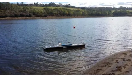
Fig. 2. The configuration of the scaled ship, Hoorn [5].
The allocation of the equipment in the model is illustrated in Fig. 2. The myRIO-1900 [11] is a real-time embedded evaluation board to drive actuators (including the rudder and twin propellers) and collect data from low-cost sensors by running LabVIEW programs. The router for the communication between offshore and onshore was installed on the model. Two motors, encoders and six batteries were installed as drag equipment. Moreover, the servo motor was employed to control the rudder at the aft.
TABLEIIDESCRIPTION OF SENSORS IN THE HOORN
Item Measurement Model
Accelerometer Surge, sway and heave
acceleration ADXL345 Gyroscope Roll, pitch and yaw rate L3G4200D Digital Compass Heading angle HMC5883L
The motions of the ship were measured by the low-cost sensors and GPS listed Table II. All the sensors were calibrated and tested in different ways before the experiments.
The free running tests were carried out in a lake in Tasmania. The standard manoeuvring tests defined by the International Towing Tank Conference (ITTC) [12] were conducted. The rudder angle was set to 10°, 20°, and 30° for the portside and starboard turning circle tests, and 20° to 20° for the zig-zag tests. The sight of proposed tests can be seen in Fig. 3.
IV. DATA PROCESSING
test of 20-degrees rudder and 540 RPM motor speed were employed for data processing and system identification.
[image:3.595.64.293.190.322.2]The data obtained from the digital compass were processed since it was more accurate and compatible with yaw angle and yaw rates for system identification than the gyroscope.
Fig. 3. Condition in the experiment site.
The noisy raw data from the free running test fit into a smooth curve using a spline function by minimizing the Penalized Sum of Squares (PSS). The first term indicates the usual sum of squares and the second term defines a roughness penalty [13].
2 2 2
( ) (1 ) d s2
PSS p y s xi i p dx
dx
(6)
where p is the specified smoothing parameter, yi is the raw
[image:3.595.56.301.526.675.2]data, and s(x) is the smoothing spline. The smoothing parameter, p was determined to 0.9 and 0.998 for each test which smoothing the raw data reasonably. The smoothed data by the method are compared to the raw data in yaw rate as shown in Fig. 4.
Fig. 4. Smoothed yaw rate of the 20-degrees turning circle test. The smoothed data are to be used for the system identification to compute the unknown coefficients and complete the proposed models in the next section.
V. SYSTEM IDENTIFICATION
The K, T1 and T2 were estimated using the measured data in matrix form by the Least Square Method through
MATLAB [14]. The second model can be expressed as
1
1 2 1 2
T T T T
r r r
K K K
(7) And it can be expressed in matrix form as below [15].
1 2
1 2
1
T T K
T T
r r r K
K
(8)
The constant vector
can be calculated by (8).( ) ( )
inv
(9) Then, the estimated coefficients for the turning circle test were calculated to T11.5205, T2 3.7887, and
0.5501
K . Therefore, the identified 2nd order model in the transfer function form was calculated as
( ) 0.5501
1.5205 1 3.7887 1
s
r
s s
(10)And the identified 1st order model in transfer function was computed as
( ) 0.5501
5.3092 1
s
r
s
(11) Furthermore, the estimated coefficients for the zig-zag test were calculated to T10.1766, T2 4.1985, and
0.6338
K . Therefore, the identified 2nd order model in the transfer function form was calculated as
( ) 0.6338
0.1766 1 4.1985 1 s
r
s s
(12)
And the identified 1st order model in transfer function was computed as
( ) 0.6338
4.3731 1
s
r
s
(13)
VI. SIMULATION AND VERIFICATION
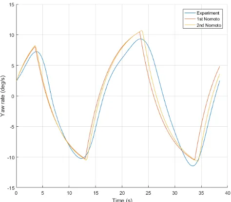
The identified models were transferred to the state space forms to set the initial values, and the speed of the ship for the turning circle test was calculated to be 1.46m/s from the trajectory and running time. The models were simulated through Simulink [14] for the same time as the experiment. The compared yaw rates between the experiment result and simulation result of the turning circle test were shown in Fig. 5. It can be noticed that the experimental data and the simulation result have a good agreement. Furthermore, the 2nd order model showed the faster turning response than 1st order model due to the additional term, T1T2 in the function.
degrees per second respectively. It should be noted that, a disagreement was found from the start to 10 seconds, it can be explained by the unknown current generated by the wind at the experimental site.
Fig. 5. Comparison in yaw rate between the experimental data and simulated data of the 20-degrees turning circle test.
[image:4.595.324.552.211.403.2]The trajectories between the experiment result and simulation results were compared as shown in Fig. 6. The 2nd order model displayed much more agreement with the experimental data than the 1st order model due to the faster response.
Fig. 6. Comparison in trajectory between the experimental data and simulated data of the 20-degrees turning circle test.
Furthermore, the compared heading angle between the experiment result and simulation results of the zig-zag test were shown in Fig. 7 and Fig. 8. Generally, the both simulation results showed faster turning response than the experimental result due to the current in the lake. It can be
noticed that the experimental data and the simulation results have small disagreements in the maximum angle at the first turning, but the figure showed great agreements in the maximum angle since the second turning as shown in Fig. 7. Furthermore, the 2nd order model showed more agreement in terms of the maximum values and respond than the 1st order model due to the due to the additional term, T1T2 in the
[image:4.595.70.286.470.688.2]function.
Fig. 7. Comparison in heading angle between the experimental data and simulated data of the 20-degrees zig-zag test.
The yaw rates between the experiment result and simulation results were compared as shown in Fig. 8. They showed less agreement than the heading angle in the maximum value due to the influence from the current. Moreover, the 2nd order model had a better agreement than the 1st order model in terms of the turning response.
Fig. 8. Comparison in yaw rate between the experimental data and simulated data of the 20-degrees zig-zag test.
[image:4.595.322.559.520.728.2]order Nomoto models can predict them more accurately than the 1st order model.
VII. CONCLUSION
This paper suggested a new method to develop the Nomoto mathematical models by employing free running test with low-cost sensors. The mathematical models were developed and the unknown coefficients were estimated successfully by the Least Square Method and smoothened data using the smooth spline method. The simulation results validated the identified parameters compared with experimental data although environmental conditions generated some uncontrollable disturbances. Furthermore, the 2nd order Nomoto model agreed with the experimental data much more than the 1st order model due to more accurate responsiveness generated from the term, T1T2. Thus,
it can be stated that the 2nd Nomoto model is more appropriate to predict the behaviour of the model scaled vessel.
For the further study, repetitive free-running tests would be demanded in order to acquire more correct data. Furthermore, the sensitivity and accuracy of all the sensors would be adjusted and improved. In addition, more experiments with less experimental disturbances would be conducted.
ACKNOWLEDGMENT
The authors wish to express thanks to Michael Underhill and Jock Ferguson of Australian Maritime College (AMC) for all the assistance with the experiments. This research would not have been completed well without their efforts.
REFERENCES
[1] L. Moreira and C. Guedes Soares, "Autonomous Ship Model to Perform Manoeuvring Tests," Journal of Maritime Research, vol. VIII, no. 2, pp. 29-46, 2011.
[2] M. Araki, H. Sadat-Hosseini, Y. Sanada, N. Umeda and F. Stern, "System Identification using CFD Captive and Free Running Tests in Severe Stern Waves," in Proceedings of the 13th International Ship Stability Workshop, Brittany, 2013.
[3] S. Phillips, I. Shin, C. Armstrong and D. Kyle-Spearman, "Instrumented Free-running Model Tests - Their Application to Small High Speed Craft," Surveillance, Search and Rescue Craft, vol. 8, no. 1, pp. 20-21, 2013.
[4] N. Im and J. Seo, "Ship Manoeuvring Performance Experiments Using a Free Running Model Ship," International Journal on Marine Navigation and Safery of Sea Transportation, vol. IV, no. 1, pp. 1-5, 2010.
[5] F. J. Velasco, E. Revestido, E. López, E. Moyano and M. Haro Casado, "Simulations of an Autonomous In-scale Fast-ferry Model," International Journal of Systems Applications, Engineering & Development, vol. 2, no. 3, pp. 114-121, 2008.
[6] D. Moreno-Salinas, D. Chaos, J. M. d. l. Cruz and J. Aranda, "Identification of a Surface Marine Vessel Using LS-SVM," Journal of Applied Mathematics, vol. 2013, no. Hindawi Publishing Corporation, p. 11, 2013.
[7] T. I. Fossen, Guidance and Control of Ocean Vehicles, New York: John Wiley & Sons, 1994.
[8] M. Fujino and N. Daoud, "Investigation into Ship Maneuverability in Shallow Water by Free-running Model Tests," The Univercity of Michigan, Ann Arbor, 1978.
[9] K. Nomoto, "Paper 1. Problems and Requirements of Directional Stability and Control of Surface Ships," Journal of Mechanical Engineering Science, vol. 14, pp. 1-5, 1972.
[10] N. S and V. Manikandan, "Model Predictive Controller for Ship Heading Control," International Journal of Industrial Electronics and Electrical Engineering, vol. 2, no. 6, pp. 6-10, 2014.
[11] National Instruments, "LabVIEW myRIO 2014, version 14.0, software," Austin, 2013.
[12] ITTC, "Full Scale Manoeuvring Trials Procedure," ITTC, Kongens Lyngby, 2002.
[13] G. Rodriguez, "Smoothing and Non-Parametric Regression," Princeton University, Princeton, 2001.
[14] MathWorks, "MATLAB R2016a, version 9.0.0.341360, software," Natick, 2016.
![Fig. 2. The configuration of the scaled ship, Hoorn [5].](https://thumb-us.123doks.com/thumbv2/123dok_us/8409559.327454/2.595.322.559.181.386/fig-configuration-scaled-ship-hoorn.webp)