Extending space time with property

(1)

University of Tasmania School of Physical Sciences

Extending Space-time with Property

Paul Stack

October 2014

Supervisors: Dr. Peter Jarvis Em. Prof. Robert Delbourgo

(2)

(3)

Declaration of Originality

This thesis contains no material which has been accepted for a degree or diploma by the University or any other institution, except by way of background information and duly

ac-knowledged in the thesis, and to the best of my knowledge and belief no material previously

published or written by another person except where due acknowledgment is made in the text of the thesis, nor does the thesis contain any material that infringes copyright.

Signed:

(4)

(5)

Authority of Access

The publisher of the paper summarising Chapter 4 and 5 hold the copyright for that content, and access to the material should be sought from the respective journals. The remaining

non published content of the thesis may be made available for loan and limited copying and

communication in accordance with the Copyright Act 1968.

Signed:

(6)

(7)

Statement of Co-Authorship

The following people contributed to the publication of work undertaken as a result of this thesis:

Paper based onChapter 4: Where-When-What: the general relativity of space-time-property

Authors:

Candidate: Stack, P.D.,School of Physical Sciences, University of Tasmania Author 1: Delbourgo, R., University of Tasmania

Candidate was the secondary author on the paper with Author 1 writing most of the wording. The content of the paper in terms of equations was done primarily by the Candidate, with

some by Author 1. Similarly the derivation of these equations in Mathematica was done

solely by the candidate. The development of the background formalism was shared between the Candidate and Author 1, with some assistance from Dr. Peter Jarvis who also provided

feedback and suggestions along the way. In terms of the content present in Chapter 4 of this

thesis, the Candidate was responsible for nearly all of it, except the section on Matter fields at the end.

Paper: Candidate (50%), Author 1 (50%).

(8)

Authors:

Candidate: Stack, P.D.,School of Physical Sciences, University of Tasmania Author 1: Delbourgo, R., University of Tasmania

Candidate was the primary author on the paper, writing it, providing equation content and

deriving the content using Mathematica. Author 1 provided feedback and contributed to the writing and content. The development of the formalism was again shared between the

Candidate and Author 1, with some assistance from Dr. Peter Jarvis. In terms of the content

present in Chapter 5 of this thesis, the Candidate was responsible for nearly all of it, except the section on Matter fields at the end.

Paper: Candidate (70%), Author 1 (30%).

Thesis chapter: Candidate (90%), Author 1 (10%).

Signed:

Dr. Peter Jarvis Prof. John Dickey Supervisor Head of School

School of Physical Sciences School of Physical Sciences

University of Tasmania University of Tasmania

(9)

Abstract

Space-time does an excellent job of describing a “when” and “where” of an event; however it fails to describe “what” was involved. Normally this is achieved by including quantum fields

with their own labels and associated properties. Conservation of these properties is then

achieved according to what experiment dictates. We propose to add additional coordinates to space-time that describe the “what” which is missing. We choose these coordinates to

be complex anti-commuting Lorentz scalars and attach various quantum numbers to them

as indicated by experimental observation. With 5 such coordinates we can accommodate all known particles in the Standard Model and can reduce the number of fundamental parameters

involved. We also develop formalism to deal with the inclusion of these coordinates into

general relativity, and look at the cases of 1 and 2 property coordinates. This results in the Einstein-Maxwell equations for 1 coordinate and the Einstein-Yang Mills equations for 2

coordinates. The Mathematica code used in this thesis, which was essential for the algebraic

(10)

(11)

Acknowledgments

Firstly I would like to thank my supervisors Bob and Peter for their continuous guidance over the last few years. Bob’s enthusiasm really made this feel like a group project, where

every result I got really mattered. The weekly meetings provided motivation but I never felt

like I was under high pressure, which made the whole process highly enjoyable and engaging. Next I would like to thank my peers, in particular Courtney, Dave and Vasaant for keeping

office life interesting and putting up with my fairly sketchy attendance. Perhaps some days

we weren’t the most productive, but those days were also the most fun. I would also like to thank the department in general for their support over the years, in particular Simon, Karen

and J.D. for always making time to help me when I had administration related issues. Lastly

but certainly not least, I would like to thank my family for their unconditional support and care over the years. They were my rock, though their support meant everything always went

so smoothly I never needed a rock.

(12)

(13)

Introduction

This thesis outlines an attempt to unify gravity with the other forces as well as explain some

aspects of of the Standard Model of particle physics. We do this by introducing complex anti-commuting Lorentz scalar coordinates into space-time. We assign to these coordinates

“property” or attribute, for example charge, isospin, colour etc. Particle fields are then

obtained by considering products of these coordinates and we can construct superfields by performing series expansions in the property coordinates. Conservation of property in

inter-actions is then achieved by performing Grassmann integration over the property coordinates,

rather than by needing to explicitly enforce conservation laws. The introduction of these coor-dinates results in a space-time-propertyZ2 graded manifold. We develop a systematic way of

tackling this in terms of general relativity and then apply this to 1 and 2 property coordinates.

The rest of this thesis fills in the details of the above paragraph. Chapter 1 will discuss

the Standard Model of particle physics, some other models like Kaluza-Klein theory and

supersymmetry and then describe the previous work that has been done on property coor-dinates. Chapter 2 will more formally introduce the property coordinates and explain how

superfield expansions can be done, resulting in mass matrices for particles. Chapter 3 covers

the systematic development of general relativity on aZ2 graded manifold. In Chapters 4 and 5 we look at introducing 1 and 2 property coordinates to space-time and the resulting field

equations. The outcome of this is a unification of gravity with electromagnetism and then SU(2) Yang Mills.

1.1 The Standard Model

The Standard Model of particle physics is tried and tested and provides us with the ability

to calculate the results of particle physics experiments to high levels of accuracy. There are many textbooks that discuss the Standard Model, for instance Griffiths (2008) provides a

solid introduction starting at a basic post-graduate level and Srednicki (2007) is a bit more

advanced and covers the basics of quantum field theory. Here we will just discuss some points

(18)

of the Standard Model that are relevant to the work done in this thesis.

The standard model is based on the gauge group SU(3) ×SU(2)L ×U(1). Each of these groups in the product have their own associated coupling constant and gauge bosons mediating the corresponding force. The strong nuclear force is mediated by 8 gluons which are

the gauge bosons of theSU(3) colour group, the weak nuclear force is mediated by the three

W±andZ bosons which are gauge bosons of theSU(2)Lgroup, and finally electromagnetism is mediated by the photon of the U(1) group. There is one other boson under the standard

model, the Higgs boson, which will be discussed soon. The fermions are as follows:

6 Leptons: e µ τ + antiparticles

6 Neutrinos: νe νµ ντ + antiparticles 18 “Up” quarks: u c t ×3 colours + antiparticles 18 “Down” quarks: d s b ×3 colours + antiparticles

This results in a total of 61 elementary particles. Note the repetition in sets of 3; 3 types

of lepton, 3 types of neutrino, 3 types of each of the quarks, this repetition is referred to as generations. Each successive generation is more massive than the previous generation, except

possibly for neutrinos where the masses aren’t yet known precisely. The latter generations of particles (except neutrinos) decay very quickly down to the lighter first generation, so in

everyday life we only come across matter that is composed of electrons, Up quarks and Down

quarks.

It should be noted that theL inSU(2)L refers to the fact that the weak force only acts

on left handed particles. This means that the νR and νL neutrinos, which are both right

handed, do not interact at all under the standard model. Originally there was a question as to whether or not they existed, however neutrino oscillations have been observed which

firstly indicates neutrinos have mass, and that these sterile non-interacting neutrinos exist as

well. However this is under the assumption that neutrinos are Dirac fermions like the other fermions in the standard model. It is also possible that neutrinos are Majorana fermions,

where the anti particle is the same as the particle. This removes the need for sterile neutrinos

but also removes the distinction between matter and antimatter. The question of whether neutrinos are Dirac or Majorana is still an open question today.

Under the Standard Model, particles get their masses via the Higgs mechanism. The Higgs

mechanism makes use of spontaneous symmetry breaking. As a demonstration consider the following Lagrangian for a scalar field φ:

2L= (∂φ)2+µ2φ2−1

2λ

2_φ4 _(1.1)

This Lagrangian has a spontaneously broken Z2 symmetry, resulting in a non-zero classical

expectation value for the scalar field of φ=±µ_λ. The Higgs mechanism involves electro-weak spontaneous symmetry breaking by considering a complex scalar Higgs doublet and enforcing

a local left handed SU(2)L gauge symmetry with a Lagrangian similar to the one above, this

(19)

1.2. KALUZA-KLEIN THEORY 3

Other fermions can then get their masses via interaction with the Higgs field. This

interaction between a Dirac field and a scalar field is called a Yukawa interaction. The

Lagrangian for a fermionψ of mass m with a Yukawa term is:

L=iψ /¯∂ψ−mψψ¯ −αφψψ¯ (1.2) The coupling strength αis different for each type of fermion. Ifφhas a non zero expectation value, for example like theφin Equation 1.1 then it can be rewritten in terms of shifted field

η =φ+µ_λ. The Yukawa term in Equation 1.2 then becomes a mass term plus an interaction

term, resulting in the following Lagrangian for the fermionic field:

L=iψ /¯∂ψ−αµ

λψψ¯ −αηψψ¯ (1.3)

The mass term from Equation 1.2 has been dropped, as it is now replaced by the term resulting from the expectation value of the scalar field φ. Note however that while this

gives us a mechanism for giving fermions mass, since each fermion has its own coupling α to

the scalar Higgs field it doesn’t allow us to calculate the masses of fermions or reduce the number of free parameters. When considering the full Standard Model Lagrangian we have

6 quarks, 3 leptons, 3 neutrinos and the Higgs Boson each of which has its own mass; there

is also the CKM quark mixing matrix and the MNS neutrino mixing matrix each of which is described by 4 parameters and finally 3 coupling constants for electromagnetism and the

strong/weak nuclear forces. This results in at least 24 parameters that have to be determined

experimentally.

The Standard Model is incapable of explaining why we observe 3 generations of particles, nor does it give any hints as to whether there are more. There are also no candidates for

Dark matter in the Standard Model, which is the current leading explanation for galactic

rotation curves. The large number of parameters along with the open questions regarding the Standard Model leads many to think there must be some underlying theory that produces

the Standard Model. Gravity is not included in the Standard Model either. Though this poses

its own set of challenges, there is no solid theory of quantum gravity yet. Unifying gravity with the other forces has been attempted in the past and one of the most notable attempts

is that of Kaluza-Klein theory.

1.2 Kaluza-Klein theory

Kaluza-Klein theory involves attaching an extra spatial dimension to space-time in an attempt

to unify gravity and electromagnetism. The original papers by Kaluza and Klein in 1921 and 1926 are in German, however Overduin and Wesson (1997) provides an introduction and

review of Kaluza-Klein theories. The additional spatial dimension is typically compactified

(20)

dimension does not directly appear in the laws of physics. The starting point for Kaluza-Klein

is to choose a form for the metric in 5 dimensions as follows:

GM N =

gmn+k2φ2AmAn kφ2Am

kφ2An φ2

!

(1.4)

We have used some slightly non-standard notation here, to be consistent with the notation

used later in this thesis. The 5 dimensional metric is written as GM N, where capital letters

M, N, etc run over 1 to 5. The 4 dimensional metric is written as gmn, where lower case letters m, n, etc run over the standard space-time dimensions 1 to 4. φis a scalar field and

Am is the gauge field for electromagnetism with scaling factor k. We take this metric and

then consider the gravitational part of the Einstein-Hilbert action:

S = 1

2κ

Z √

−G R d5x (1.5)

where R is the 5 dimensional Ricci “superscalar” and√−G is the volume element on the 5 dimensional manifold. If we consider the case where φ= constant, which is essentially what will be done later in this thesis, variation of this action produces the following field equations:

Rmn− 1

2GmnR= 1 2k

2_φ2_T

mn (1.6)

Fmn;n= 0 (1.7)

where Tmn = FmsFsn− 1₄gmnFklFkl is the electromagnetic stress-energy tensor. The first of these equations is the Einstein field equations for electromagnetism. Without explicitly

including gauge fields in the action we now have the gauge fields appearing correctly as a part of the geometry. The second of these equations is the Maxwell equations in curved space. The

result of all this is that in the case of pure electromagnetism we now have the equations that

govern both gravity and electromagnetism produced by considering a single action, in effect unifying those forces. Work has also been done on higher dimensional Kaluza-Klein theories in

an attempt to unify the other forces with gravity as well. One of the issues with Kaluza-Klein

theories is the infinite number of Fourier modes in the 5th coordinate, potentially resulting in an infinite number of particles with increasing mass. Kaluza got around this by only

considering the ground modes, but this causes problems for higher dimensional Kaluza-Klein

theories that make use of compactification.

1.3 Georgi-Glashow SU(5) model

The Standard Model is a gauge theory based on the group SU(3)×SU(2)L×U(1), with 3 separate coupling constants for the SU(3) colour force, SU(2)L weak force, and U(1)

electromagnetism. Georgi and Glashow (1974) proposed a model to unify these forces with 1

(21)

1.4. EXTENDED GENERAL RELATIVITY 5

group of the Standard Model. The Standard Model we observe is due to a spontaneous

symmetry breaking of the overall SU(5) group, resulting in the Standard Model for low

energies. Particles are fitted into various representations of SU(5), though this model also predicts some other particles like super-heavy coloured vector bosons. The presence of these

bosons allows the proton to decay, which is disallowed under the Standard Model. The fact that they are super-heavy means the lifetime of the proton is quite long; however experiments

have been performed to measure the decay rate of the proton and no decays have been

observed. Clark (2007) for instance looked for proton decays in 4 different channels and found the lifetime of the proton has to be at least order 1033 _{years, which essentially rules}

out the original Georgi-Glashow model. The model is still worth mentioning however as it is

used as the basis for several modern theories which have greatly increased proton half-lives. For a review of grand unified theories, including SU(5), SO(10) andSU(2)×SU(2)×SU(4) see Baez and Huerta (2010).

1.4 Extended General Relativity

Attempts to unify gravity with the other forces in a manner similar to Kaluza-Klein by extending general relativity on a higher dimensional supermanifold have been studied quite

extensively. This work makes extensive use of concepts from topology, like fibre bundles on

differential manifolds. Trautman (1970) provides an introduction to these ideas aimed at physicists, and then suggests how they can be used to extend Kaluza-Klein theory to non

abelian groups. These ideas are used by several authors to attempt to unify the non abelian

gauge forces with gravity. For instance Cho (1975) extends Kaluza-Klein type unifications by using non abelian gauge fields, and produces an Einstein-Hilbert action which results in the

unification of gravity with a non abelian gauge field plus a cosmological constant. Tabensky

(1976) takes a slightly different approach, but produces a similar result. Tabensky (1976) also notes that they have spin-1 bosons of the Yang-Mills type and spin-0 bosons, which are

coupled to spin-2 gravitons, but no fermions. One way to introduce fermions in a theory

like this is by including transformations that mix fermions and bosons, this is what leads to supersymmetry.

1.5 Supersymmetry

Supersymmetry is currently one of the leading areas of research into physics beyond the Standard Model. Zee (2010) provides an introductory chapter on supersymmetry; some of

the basic concepts will be outlined here. The underlying idea behind supersymmetry is to

introduce a symmetry between bosons and fermions. Currently we do not observe any such symmetries in nature, but this doesn’t necessarily mean they don’t exist at some higher

energy our accelerators have not managed to reach yet. The first step is to define some

(22)

In extended supersymmetry there are N of these generators. Increasing N results in more supersymmetry, which constrains the field content. For N > 8 there are massless fields of spin >2 that are produced, which cause issues for the theory. As a result of this N = 8 is considered to be maximally supersymmetric. We will now look atN = 1 supersymmetry, for which we have the following commutation relations:

[Pµ, Qα] = 0 (1.8)

[Jµν, Qα] =−i(σµν)αβQβ (1.9) [Jµν,Q¯α˙] =−i(¯σµν)α˙_β˙Q¯

˙

β _(1.10)

n

Qα,Q¯_β˙

o

= 2(σµ)_α_β˙Pµ (1.11)

{Qα, Qβ}=

n

¯

Qα˙,Q¯_β˙

o

= 0 (1.12)

These operators are independent of space-time coordinates, and so commute with the

momentum operator Pµ, giving the first commutation relation. They transform as Weyl spinors, which gives the second and third commutation relations with the Lorentz generators

Jµν. The last two lines give the supersymmetry algebra, which essentially comes out as the

only possibility for the Grassmann Qα.

The momentum operator can be thought of as generating translation in space-time. The

corresponding idea for supersymmetry generators would be to generate translation in some Grassmann coordinates θα and ¯θβ˙. This leads to the concept of a superspace, with

coordi-nates (xµ, θα,θ¯β˙). The xµ are the standard space-time coordinates and are bosonic, the θα

and ¯θβ˙ are fermionic and transform as 2 component Weyl spinors. Superfields can then be constructed on this superspace, Φ(xµ, θα,θ¯β˙).

One can also define operators Dα and ¯D_β˙ which anticommute with Qα and ¯Q_β˙. A superfield that satisfies ¯D_β˙Φ = 0 is called a chiral superfield. We can then define

yµ= (xµ+iθα(σµ)αα˙θ¯α˙), which satisfies ¯D_β˙yµ = 0. Thus if we have a superfield Φ(yµ, θα),

that depends only on y and θ it will automatically satisfy ¯D_β˙Φ = 0 and hence be a chiral superfield. When constructing Φ(y, θ) we perform a power series expansion in θ. As these

are two component Grassmann objects the highest power possible is θθ, the power series

terminates here. Thus Φ(y, θ) takes the form:

Φ(y, θ) =φ(y) +√2θψ(y) +θθF(y) (1.13) This superfield contains a Weyl fermion field ψ as well as two complex scalar fields, φ and

F. This superfield can be used to construct an action invariant under supersymmetry. One

example action is as follows:

S =

Z

d4x

h

Φ†Φi D

−[1 2mΦ

2₊1 3gΦ

3_]

F +

[1 2mΦ

2₊1 3gΦ

(23)

1.6. PROPERTY COORDINATES 7

where [X]D refers to only using the θθθ¯θ¯coefficient, [X]F refers to only using the θθ

coeffi-cient. This action can then be used to find the equations of motion for the fields and their

interactions.

While supersymmetry is one of the leading areas of research into physics beyond the

Standard Model, we have not yet discovered any experimental evidence for it. The data from

the LHC has been used to search for supersymmetric partners to known particles but so far nothing has come up, forcing theorists to keep raising the mass of the lightest superpartner

in their theories. Even those involved in the research of supersymmetry are starting to ask at what point should we give up on it. The fact that supersymmetry hasn’t worked out so

far means searching for alternative theories warrants serious consideration. This thesis is an

attempt to develop one of these theories, which borrows some ideas from the other theories discussed here but is different to anything done before.

1.6 Property coordinates

We now reach the model considered in this thesis. The following section will consist of two

aspects, first describing the historical development of the theory and then secondly describing its state before the commencement of this thesis. This will allow us to then demonstrate the

original work carried out in this thesis extending work on the model. The specific details

of the theory will be described in later chapters, so as to allow a consistent build up of the concepts involved.

One of the first papers considering the addition of Grassman coordinates to spacetime

is Arnowitt and Nath (1976). Using some of the ideas of supersymmetry Grassman coor-dinates are included in spacetime and local gauge symmetry is applied. By considering the

Einstein-Hilbert Lagrangian, this results in unification of gravity with electromagnetism. The

work by Arnowitt and Nath (1976) is later expanded upon by Delbourgo and Zhang (1988a), Delbourgo et al. (1988) and Delbourgo and Zhang (1988b). These papers consider including

5 complex Grassmann variables ζ to the standard 4 of space-time to produce the Standard

Model and also the possibility of unifying gravity and the other forces. Particles are repre-sented by monomials in these coordinates, with the observed particles of the Standard Model

accommodated easily. There were however a reasonably large excess of particle states, some of which produced anomalies. Delbourgo and White (1990) suggested a method of cutting

down on these states via self-duality. This was implemented by Delbourgo et al. (1991) to

reduce the number of particle states for the 5 coordinate model; the anomalies could be dealt with while still having enough room for the Standard Model. Delbourgo et al. (1993)

con-sidered in detail the various Lie algebras and representations that could be constructed from

N Lorentz scalar Grassmann variables and their derivatives. Two models with N = 5 were considered and by applying duality restrictions both were made anomaly free. The first took

odd monomials (products of an odd number of Grassmann coordinates) to be right-handed

(24)

Delbourgo (2006a) associated the 5 Grassmann coordinates with specific quantum

num-bers, like charge and fermion number, making them carriers of the property of particles. The

assignments are as follows:

Property coordinate: ζ0 ζ1 ζ2 ζ3 ζ4

Charge (units of e): 0 1/3 1/3 1/3 -1

Fermion number: 1 -1/3 -1/3 -1/3 1 Colour: None Red Green Blue None

Fermions are made up from odd monomials in the property coordinates and bosons are

made up from even monomials. This arrangement preserves spin-statistics. A self-duality

restriction is then applied to reduce the number of particle states and to eliminate anomalies. The resulting fermions include 3 up-type quarks, 8 down-type quarks, 6 charged leptons, 4

neutrinos and a corresponding set of antiparticles. The fermions of the Standard Model are

accommodated, along with some extra particles that have not been observed yet. There are also 9 Higgs-like neutral scalars. These could in theory impart masses to the fermions via

their 9 expectation values, resulting in less parameters than the Standard Model. Superfields can also be constructed: Φ(x, ζ,ζ¯) is a superfield describing bosons, which contains the

even monomials in the property coordinates that survive the duality restrictions; similarly

Ψ(x, ζ,ζ¯) is a superfield describing fermions and contains the odd monomials of the property coordinates.

Unification of gravity with electromagnetism was also attempted in this paper, by

con-sidering general relativity with 1 property coordinate. However rather than appending one complex anti-commuting Lorentz scalar ζ and its conjugate ¯ζ to space-time, two real

coor-dinates (ξ, η) were considered instead. Two supermetrics GM N were considered, the first

includes curvature in the property sector but no gauge fields:



 

Gmn Gmξ Gmη

Gξn Gξξ Gξη

Gηn Gηξ Gηη

  =   

gmn(1 +if ξη) 0 0

0 0 −iΛ2(1 +igξη) 0 iΛ2(1 +igξη) 0





 (1.15)

The Einstein-Hilbert action produced from this metric included the standard gravitational

action plus a cosmological constant. The other supermetric considered involved gauge fields but no property sector curvature:



 

Gmn Gmξ Gmη

Gξn Gξξ Gξη

Gηn Gηξ Gηη

  =   

gmn(1 +if ξη) + 2iΛ2ξAmAnη iΛ2Amξ iΛ2Amη

iΛ2Anξ 0 −iΛ2

iΛ2Anη iΛ2 0





 (1.16)

This supermetric produces an Einstein-Hilbert action containing the gravitational curvature plus the electromagnetic Lagrangian. The inclusion of the gauge fields in the space-property

section of the supermetric is similar to the Kaluza-Klein model, with a similar result as well,

(25)

1.7. ORIGINAL THESIS WORK 9

Some formalism for considering general relativity on a graded manifold was also developed

in this paper. However there were some small self-consistency issues that will be elaborated

on in Chapter 3 of this thesis.

Delbourgo (2006b) considered the Yukawa interactions present in model from Delbourgo (2006a). The 9 neutral Higgs fields are assumed to have independent expectation values,

resulting in an expectation value for the Higgs superfield hΦi. Flavor mixing and mass matrices are produced by considering a Yukawa term of the form:

Z

d5ζd5ζ¯Ψ¯hΦiΨ (1.17) Terms from this expansion can then be selected to give flavor mixing matrices, 8×8 for down quarks, 6×6 for leptons etc. An attempt was made to give numerical values for the 9 Higgs expectation values to see if a sensible mass spectrum could be obtained. While the quark masses were satisfactory, the mixing matrices didn’t work out so well, nor the masses of the

light leptons. The possible space of values was not searched completely, so there is still room

for the model to work out. If the duality restriction were dropped from the Higgs superfield Φ then there would be 18 possible Higgs expectation values to play with, however this is

nearly as many parameters that the Standard Model has in the first place!

1.7 Original Thesis work

This thesis updates, verifies and builds on the previous work regarding property coordinates. Here we will outline the original research conducted as a part of this thesis.

The most significant contribution is the development of Mathematica code designed to

deal with the large amount of algebra required. Previous work on property coordinates had

been done by hand, which limited what could be achieved. Many of the results found in this thesis would not have been possible without the significant amount of time invested into

developing Mathematica code. The code itself is available from the UTAS library digital

repository and is discussed in Appendix B.

The 9 Higgs fields mentioned in Delbourgo (2006b) have their expectation values treated as independent variables, when in theory they should be produced by spontaneous symmetry

breaking. In this Chapter 2 we perform the algebra to determine the spontaneous symmetry

breaking for the Higgs fields. For a renormalisable theory this requires evaluation of Φ2, Φ3 and Φ4, where Φ is the superfield expansion containing the 9 Higgs fields. These are used

to produce the Higgs potential which is then minimised to get conditions on the expectation

values of the Higgs fields. The number of parameters in the model is greatly reduced by this process, as all fermion masses are then dependent on the 3 parameters in the Higgs

Lagrangian instead of the 9 Higgs expectation values.

Delbourgo (2006a) included a section outlining how to deal with general relativity on a

(26)

this thesis, however there are some issues with the formalism developed in that paper. The

formalism is re-derived in Chapter 3, with several checks performed for self-consistency.

That paper also looked at General Relativity with 1 property coordinate. However instead of using a complex Grassmann coordinate and its conjugate, 2 real coordinates were used.

Since the algebra involved was so difficult to perform by hand two separate cases were consid-ered, a supermetric with curvature in property only and another with gauge fields only. These

were also only determined in the case of Minkowski space-time, the gravitational factors were

then included by assuming the tensors had to be generally covariant. Chapter 4 considers the case of 1 property coordinate included in space-time, but does so with complex Grassmann

coordinates, developing the formalism required. A general supermetric is used that includes

both curvature in the property sector and gauge fields at the same time. Using the Mathe-matica code developed, the Einstein-Hilbert action is then determined in the general case of

curved space-time. The field equations are also considered for both space-time and the gauge

field. This is all repeated in Chapter 5, except with 2 property coordinates. The additional formalism required to deal with non-abelian gauge fields as well as the supermetric, resulting

Einstein-Hilbert action and field equations are all included.

The vast majority of the remaining sections of this thesis represent original research. The parts that are repeated from Delbourgo (2006a) and Delbourgo (2006b) are re-derived to

(27)

Chapter 2

Property coordinates, Superfields

Space-time forms a solid framework in which we can describe the position and time of events

and interactions. We can also describe the momentum and energy transfers that occur in these events, but when it comes to describing the properties of the particles and fields involved

space-time falls short. Usually we just assign some external labels to specify what particles

are involved in any given interaction, but what if we didn’t have to do this? The focus of this thesis is to see what happens when extra coordinates are appended to space-time in an

attempt to describe particle properties in one coherent framework. Note that it is assumed the reader has at least a passing familiarity with the concepts of superspaces and superfield

expansions. For background reading any good supersymmetry textbook should suffice, for

example Wess and Bagger (1992) provides an introduction to these ideas and Weinberg (2000) provides a more involved explanation.

2.1 Property model

The model presented in this thesis is constructed as follows:

1. We attach to space-time N complex property coordinates ζ = (ζ1, ζ2, ..., ζN) and their

complex conjugates ¯ζ = (ζ¯1, ζ2¯, ..., ζN¯) to form a 4 + 2N dimensional superspace X =

(x, ζ,ζ¯).

2. We choose these coordinates to be anti-commuting, ζµζν = −ζνζµ. This results in a graded superspace; the 4 dimensional space-time part is even graded and the 2N

dimensional property sector is odd graded. The property sector is an Sp(2N) group, for a detailed discussion of the group structure see Delbourgo et al. (1993).

3. Anti-commutativity also this ensures that superfield expansions will terminate with a

finite number of terms since ζµζµ =−ζµζµ, which is true if and only if ζµζµ= 0. So for example a superfield expansion with one property coordinate would take the form:

S(x) = a(x) +b(x)ζ +c(x) ¯ζ +d(x) ¯ζζ, with a, b, c and d being space-time dependent

particle fields.

(28)

4. Any term in a superfield expansion can only contain one of eachζor ¯ζ, this is also where

the idea of a property comes in, a particle can only either have or not have a particular

property associated with a given ζ or ¯ζ. Add the quantum numbers of individualζ and ¯

ζ to get the overall quantum numbers.

5. We choose to have the conjugates providing the opposite property of their type. This

leads naturally to anti-particles with complex conjugation being associated with charge conjugation, swapping between a particle and its anti-particle. Since a property and

its complex conjugate cancel each other out this also produces generations of

parti-cles, where the same quantum numbers are present but extra property/conjugate pairs change the coupling to the Higgs field and hence the masses.

6. An odd number of property coordinates is overall anti-commuting, while an even number

of property coordinates commutes. To satisfy spin-statistics we associate odd numbers of property coordinates with fermionic particle fields, and even ones with bosonic fields.

7. We choose these coordinates to be Lorentz scalar, this separates our scheme from

super-symmetry and greatly simplifies the algebra when we begin to consider general relativity on the superspace in later chapters.

We now want to know how many coordinates are required to include all known particles

from the standard model. This is done by considering superfield expansions; which are power series expansions in the property coordinates, where each term represents a particle field. It

is clear there must be at least 3 such coordinates, one for each colour to model quarks. We

can assign colour to 3 property coordinates as follows:

Coordinate ζ1 _ζ2 _ζ3

Colour Red Green Blue (2.1)

This is sufficient to model the strong force. However to produce a colourless fermionic particle,

like an electron or neutrino with an odd number of property coordinates, the only possible combination is to include all three of them, ζ1ζ2ζ3. This means we don’t have the ability to

produce both electrons and neutrinos, so we need at least 4 coordinates. The questions of whether 4 is enough is a bit more subtle, but if you assign charge and colour to 4 coordinates

it isn’t possible to produce three generations of electron, neutrino, down quark and up quark

made up ofodd numbers of property coordinates. This means we are forced to use 5 property coordinates (ζ0_{, ζ}1_{, ζ}2_{, ζ}3_{, ζ}4 _{and conjugates} _ζ0¯_{, ζ}¯1_{, ζ}¯2_{, ζ}¯3_{, ζ}¯4_{), which easily includes all the}

particles of the standard model but also many more. Let us count the number of property

coordinatesζ that make up a term in the superfield expansion and call thatp, then count the number of conjugate coordinates ¯ζ and call thatq. We can then group terms in the superfield

expansion by their corresponding (p, q) pair. The number of possible particle states for a given

(29)

2.2. NOTATION 13

Number of terms in superfield expansion of type (p,q)

p=

0 1 2 3 4 5

0 1 5 10 10 5 1

1 5 25 50 50 25 5 2 10 50 100 100 50 10

q = 3 10 50 100 100 50 10

4 5 25 50 50 25 5

5 1 5 10 10 5 1

(2.2)

For example this means there are 50 possible superfield terms and hence particles of type

(2,1), that is with 2 ζ and 1 ¯ζ present.

2.2 Notation

Before considering our model further we first need to establish some notational convention. Products of ζ and their conjugates ¯ζ will appear frequently in this chapter. To reduce the

amount of space taken up, and to allow a clearer picture of what is going on, a shorthand

notation will be used. First the products are arranged into a canonical order; with ζµ’s arranged into increasing order of µ followed by the conjugate coordinates ζµ¯ arranged in

increasing order of ¯µ. This arrangement can always be done as the coordinates anti-commute

with each other, with a sign produced depending on the sign of the permutation required to form the canonical order. For example:

Unordered Product Ordered Product

ζ2ζ3ζ1 =ζ1ζ2ζ3

ζ¯1ζ2ζ3ζ4 =−ζ2ζ3ζ4ζ¯1 (2.3)

ζ¯4ζ1ζ¯3ζ¯2ζ¯1 =−ζ1ζ¯1ζ¯2ζ¯3ζ¯4

The repeated ζ and ¯ζ do not provide any useful extra information, so the product can be written in shorthand removing these repeated symbols. For example:

Full product Shorthand (2.4)

ζ1ζ2ζ3 =ζ123 (2.5)

ζ2ζ3ζ4ζ¯1 =ζ234¯1 (2.6)

ζ1ζ¯1ζ¯2ζ¯3ζ¯4 =ζ1¯1¯2¯3¯4 (2.7)

This process can always be reverted by simply filling in the missing ζ symbols. Finally

(30)

R

dζ = 0,R _¯

ζdζ = 0,R _¯

ζζdζdζ¯= 1 etc. See Berezin (1987); DeWitt (1984) for more

back-ground on Grassmann coordinates.

2.3 Charge conjugation

We take the charge operator cto act like a Hermitian conjugate on the property coordinates.

The order of the property coordinates is reversed and then they are swapped between ζ ↔ζ¯. This changes between particles and anti-particles as the conjugate property coordinates have

the opposite quantum numbers. For example (ζ123)c = (ζ3)c(ζ2)c(ζ1)c = ζ¯3ζ¯2ζ1¯ = −ζ¯1¯2¯3. In terms of Table 2.2 charge conjugation is represented by a swapping of p and q, so for a particle state belonging to the group (2,1) its anti-particle will belong to (1,2). This produces

a symmetry about the p = q line on the table, halving the number of fermions we have to

consider. To further reduce the number of particle states we will apply another symmetry condition we call anti selfduality.

2.4 Self duality

Following the work done by Delbourgo et al. (1991) and Delbourgo et al. (1993), we can

impose a symmetry restraint on the possible particle states using the dual operator. The

dual operator is effectively a reflection in the cross diagonal of Table 2.2, taking (p, q) to (5−q,5−p). It can be constructed from the 5-dimensional Levi-Civita as follows:

(ζa1...apb¯1...b¯q₎×₌_εa1...apap+1..a5_ε¯b1...¯bq¯bq+1...¯b5_ζbq+1...b5¯ap+1...¯a5_/₍₍₅₋_p_)!(5₋_q_)!)_. _(2.8)

Here rather than the standard Einstein summation over repeated “up” and “down” indices

we have summation over repeated indices and their conjugates (sum over ai and ¯ai, bj and ¯

bj). The factor of 1/(5−p)!(5−q)! is for counting, as there arep! ways of permutingpindices. The following table lists general forms of duals for a few example (p, q) types as well as some

specific examples:

Product Type Dual Dual type

1 (0,0) εijklm_εa¯¯b¯cd¯¯e_ζabcde¯i¯j¯k¯lm¯_/_{(5!5!) =}_ζ01234¯0¯1¯2¯3¯4 _(5,5)

ζi (1,0) εijklmε¯a¯b¯cd¯¯eζabcde¯j¯k¯lm¯/(4!5!) (5,4)

ζij¯a (2,1) εijklmε¯a¯bc¯d¯e¯ζbcde¯k¯lm¯/(3!4!) (4,3)

ζijk¯a¯b (3,2) εijklmε¯a¯bc¯d¯e¯ζcde¯lm¯/(2!3!) (3,2)

ζ123 (3,0) ε12304ε¯0¯1¯2¯3¯4ζ01234¯0¯4 = -ζ01234¯0¯4 (5,2)

ζ234¯1 (3,1) ε23401ε¯1¯0¯2¯3¯4ζ0234¯0¯1 = -ζ0234¯0¯1 (4,2)

ζ1¯1¯2¯3¯4 (1,4) ε10234ε¯1¯2¯3¯4¯0ζ0¯0¯2¯3¯4 = -ζ0¯0¯2¯3¯4 (1,4)

ζ12¯3¯4 (2,2) ε12034ε¯3¯4¯0¯1¯2ζ012¯0¯3¯4 =ζ012¯0¯3¯4 (3,3)

Note that we use the convention thatε01234=ε¯0¯1¯2¯3¯4 = 1. It is important that the dual

(31)

2.5. FIVE COORDINATE MODEL 15

can be written asζ12¯3¯4ζ0¯0, theζ0¯0 part does not change the property as it is a conjugate pair.

Since the dual operator preserves property it can be used to place a symmetry restriction on

the superfield expansions. We now require that the superfield expansions are anti selfdual. So for instance ζ12¯3¯4 would be grouped with its dual to form a single term: (ζ12¯3¯4−ζ012¯0¯3¯4) which under the dual operator changes sign. This effectively cuts the number of possible particle states from Table 2.2 in half. Terms that are selfdual are eliminated by this process,

for instance the product ζ01234 goes to itself under the dual operation, so to maintain anti

selfduality this term becomes zero. Similarly terms of the form ζ0123¯4 or ζ012¯3¯4 where there are no conjugate pairs are also eliminated.

Number of terms in superfield expansion of type (p, q) after symmetry reduction

p=

0 1 2 3 4 5

0 1 5 10 10 5 0

1 ∗ 25 50 50 10 ×

2 ∗ ∗ 100 45 × ×

q = 3 ∗ ∗ ∗ × × ×

4 ∗ ∗ ∗ ∗ × ×

5 ∗ ∗ ∗ ∗ ∗ ×

(2.9)

The * are the anti-particles and the × are equivalent under the anti selfduality condition. Delbourgo et al. (1993) go into more detail regarding how the duality and charge operators

arise from the algebra of Lie group automorphisms, though the actual model we use is similar

to Delbourgo (2006b).

2.5 Five coordinate model

Quantum numbers We can now assign quantum numbers to our property coordinates ζ and ¯

ζ

Property ζ0 ζ1 ζ2 ζ3 ζ4

Charge 0 −1/3 −1/3 −1/3 1

Colour None Red Green Blue None

Lepton Number 1 0 0 0 −1

(32)

Property ζ¯0 ζ¯1 ζ¯2 ζ¯3 ζ¯4

Charge 0 +1/3 +1/3 +1/3 −1 Colour None AntiRed AntiGreen AntiBlue None

Lepton Number −1 0 0 0 1

Fermion Number −1 −1/3 −1/3 −1/3 1 Similar to Anti Neutrino Anti Down Anti Down Anti Down Electron

(2.10)

The charge listed is in units of the charge of a proton. The above assignment of quantum

numbers is based on SU(5) and SO(10) grand unified theories, see Georgi and Glashow (1974) and Georgi (1975) for the original papers, and neatly produces all the observed particles in the

standard model. By requiring that the superfield expansions are anti selfdual some “bad”

quantum states are eliminated, for instance ζ0123¯4 which would have been a particle with fermion number 3 and charge −2. We can list where the standard model fermions appear in Table 2.9, writing: L for charged leptons, N for neutrons, D for down quarks, U for up

quarks and including c for charge conjugates.

Standard model fermions by (p, q) pair

p=

0 1 2 3 4 5

0 N1, Lc1, D1 L5, Dc7, U3

1 ∗ N2,3, Lc2,3, D2,3,4, U1c L6, Dc8, U4 2 ∗ Lc₄, N4, D5,6, U2c ×

q = 3 ∗ ∗ ×

4 ∗ ∗ ×

5 ∗ ∗ ∗

(2.11)

The above table lists the particle states similar to those of standard model particles with the

correct colour, charge and fermion number. We have 4 generations of Neutrino, 6 generations of charged Leptons, 8 generations of Down quarks and 4 generations of Up quarks. It appears

this breaks the symmetry between the Leptons, as we no longer have a neutrino paired up

with every charged lepton, but 2 of the charged “leptons” are produced by the combination

ζ123 _{which makes them have a lepton number of zero. We also have 8 generations of Down}

quarks which is excessive, but required to allow for enough generations of Up quark. There

are many other types of exotic particles present. Overall including both standard model and exotic particles, but not anti-particles, we have the following fermions:

Charge −4/3 −1 −2/3 −1/3 0 1/3 2/3 1 4/3 5/3

Count 6 20 12 6 20 30 12 2 6 6 (2.12)

This extra abundance of charged particles does provide a test for our model, by considering

(33)

2.6. SUPERFIELD EXPANSIONS 17

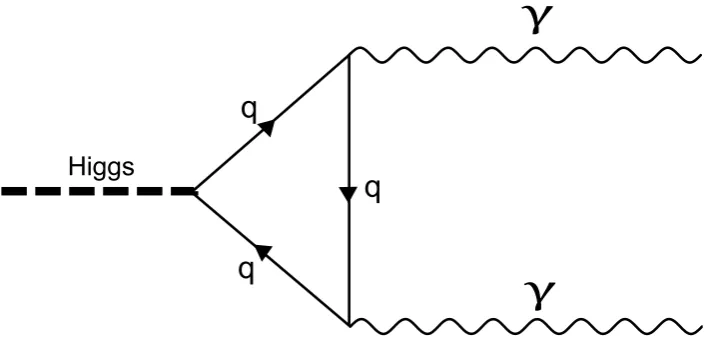
Higgs

γ

q

[image:33.595.66.420.73.246.2]

q

Figure 2.1: Higgs decay into two photons via quark loop

this decay is dependent on the charge squared of the quark in the loop and the mass of the

quark involved (Egede 1998). Only the top quark is heavy enough to provide any significant contribution under the standard model, our model however admits new particles that we

haven’t observed yet, so they must be heavier than the top. If we assume these new particles are very heavy, the mass dependence becomes weak and we can simply sum the squares of

the charges to get an estimate of the expected decay rate. Performing this for our model

gets a back of the envelope estimate of ∼10×the Higgs decay rate, however observations of the Higgs boson at the LHC indicate that the decay width to two photons is close to the

standard model rate, see ATLAS Collaboration (2014). This is evidence against our current

model, though any unified theory that introduces heavy charged fermions is going to have to deal with this issue. Note that in this analysis we have not included the loops of charged

W’s that can affect theH →2γ rate.

2.6 Superfield expansions

To construct explicit superfield expansions we perform a series expansion in the property

coordinates, multiplying each term by the corresponding space-time dependent field. We

want the superfields to have no property overall, so we match up the terms in the series expansion with particle fields that have the opposite quantum numbers. For instance ζ4

pairs with Lc not L. The last step is to include anti-particles and also the anti selfduality

condition. We will list here the superfield expansion ΨN for the neutrinos:

2ΨN = ζ

¯ 0_N

1+N1cζ0

1−ζ12341234

+ ζ¯0N2+N2cζ0

ζ4¯4+ζ123123

+ ζ¯0N3+N3cζ0

ζi¯i−ζ0¯0ζj¯jζk¯k/2

/√3 + ζ¯0N4+N4cζ0

ζi¯iζ4¯4−ζj¯jζk¯k/2

(2.13)

where the repeated indices are summed over 1, 2 and 3; for instance ζi¯i =ζ1¯1+ζ2¯2+ζ3¯3.

(34)

colour group, so for the colourless parts of the superfield expansion to be invariant under

transformations to the colour group we require the use of the SU(3) invariantζi¯i. It is useful

to note that ΨN satisfy

R

d5ζd5ζ¯( ¯ΨNΨN) = ¯N1N1+ ¯N2N2+ ¯N3N3+ ¯N4N4 as expected. The superfield expansions for the other fermions can be found in Delbourgo (2006b), and have

similar properties.

Colourless neutral bosons (Higgs-like)

p=

0 1 2 3 4 5

0 M H

1 A,B,C ×

2 ∗ D,E,F,G ×

q= 3 ∗ × ×

4 ∗ ∗ ×

5 ∗ ∗ ×

(2.14)

We can also perform a superfield expansion in colourless chargeless scalar bosons, which are Higgs-like particle fields. There are 9 such possible fields, which are shown in Table 2.14.

All of these fields can act like the Higgs if they have non-zero expectation values. If we

assume each of these fields takes on their expectation value then the full superfield expansion of the expectation value of the Higgs superfield Φ is:

2hΦi=M(1−ζ0123401234) +A(ζ0¯0+ζ12341234)

+B(ζi¯i−ζ0404ζj¯jζk¯k/2)/√3 +C(ζ4¯4−ζ01230123)

+D(ζ0¯0ζi¯i+ζ4¯4ζj¯jζkk¯/2)/√3 +E(ζ4¯4ζi¯i+ζ0¯0ζj¯jζk¯k/2)/√3 (2.15) +F(ζi¯iζj¯j/2−ζ0404ζk¯k)/√3 +G(ζ0404+ζ123123)

+ (Hζ1234+H?ζ1234)(1 +ζ0¯0).

Note that all the expectation values other than H are real. Checking this we see that 2R d5ζd5ζ¯hΦi2 = M2 ₊_A2₊_B2 ₊_C2 ₊_D2 ₊_E2 ₊_F2 ₊_G2 _{+ 2}_H?_H_{. Like the standard} model Higgs, our scalar fields can acquire non-zero expectation values via spontaneous

sym-metry breaking if we assume the following Lagrangian for the Higgs superfield:

L=

Z

d5ζd5ζ¯

(∂Φ)2/2 +µ2Φ2/2−√2fΦ3/3−gΦ4/6

(2.16)

Note the cubic term which is included for generality, the standard spontaneous symmetry breaking Lagrangian does not use it. Using Mathematica we can expand out this Lagrangian

fully and then take the variation with respect to each of the expectation values. Equating

(35)

2.6. SUPERFIELD EXPANSIONS 19

conditions are as follows:

0 =Mµ2−f

A2₊_B2₊_C2₊_D2₊_E2₊_F2₊_G2_{+ 2}_H2₊ 3M2 2

−g

− ABD − BCE −2BDE√

3 −

B2_F

√

3 − CDF − AEF − ACG − BF G − AH 2

+A2M+B2M+C2M+D2M+E2M+F2M+G2M+ 2H2M+2M 3

3

.

0 =Aµ2−f −BD − EF − CG − H2+ 2AM

−g

B2_E

√

3 +BCF − BDM − EF M − CGM − H

2_M₊_AM2

0 =Bµ2−f

−AD − CE − 2√DE

3 − 2BF

√

3 − F G+ 2BM

−g 2BCD √ 3 + 2ABE √

3 +ACF+

B2_G

√

3 − ADM − CEM −

2DEM √

3 −

2BF M √

3 − F GM+BM 2

0 =Cµ2−f(−BE − DF − AG+ 2CM)−g

_B2_D

√

3 +ABF − BEM − DF M − AGM+CM 2

0 =Dµ2−f

−AB − 2√BE

3 − CF+ 2DM

−g

B2_C

√

3 − ABM −

2BEM √

3 − CF M+DM 2

0 =Eµ2−f

−BC −2√BD

3 − AF + 2EM

−g

_AB2

√

3 − BCM −

2BDM √

3 − AF M+EM 2

0 =Fµ2−f

−B

2

√

3− CD − AE − BG+ 2F M

−g

ABC − B

2_M

√

3 − CDM − AEM − BGM+F M 2

0 =Gµ2−f(−AC − BF + 2GM)−g

B3

3√3 − ACM − BF M+GM 2

0 =Hµ2−f(−AH+ 2HM)−g −AHM+HM2

(2.17)

The Mathematica code to derive these conditions is in the associated code for this thesis.

Note that from now on we assumeHis real to help make the conditions easier to work with. This system of equations can be used to calculate the expectation values of the 9 Higgs fields

in our model. The benefit of doing all this is that we can have just one Higgs coupling, unlike

the standard model where particle masses are essentially set by their independent coupling strengths to the Higgs field. In principle particle masses are derivable from a set of algebraic

conditions, with only 3 free parameters from the Higgs superfield Lagrangian. In practice

this system is quite hard to solve, especially when coupled with the fermionic mass matrices in an attempt to derive sensible particle masses. One extra complication to consider is that

of not requiring the Higgs superfield to be anti selfdual, this would result in a doubling of the possible Higgs fields to 18. This would be a system of 18 simultaneous equations to solve,

(36)

2.7 Mass matrices

We can consider a Yukawa term describing the interaction between the fermion superfield and the Higgs superfield to get masses for fermions.

L_yukawa=

Z

d5ζd5ζ¯

¯ ΨhΦiΨ

(2.18)

Expanding this out leads to a series of terms, which can be arranged into mass matrices. The

elements of the mass matrix for a particleX are the coefficients of ¯XrXs and ¯XcrXsc, for row

r and column s. For example the Yukawa Lagrangian for neutrinos contains the following

terms:

Lyukawa ⊃(A/2 +M) ¯N1N1+ (A/2 +M) ¯Nc1N1c+ (C/2− G/2) ¯N2N1+ (C/2− G/2) ¯Nc2N1c This means the neutrino mass matrix has row 1, column 1 contain (A/2 +M) + (A/2 +M) =

A+ 2Mand row 2, column 1 contain (C/2− G/2) + (C/2− G/2) =C − G. The same pattern follows for the other terms and then other types of particle. The full set of mass matrices for the neutrinos, charged leptons, up and down quarks can be found over the page. The code

used to derive them is available in the associated code with this thesis. A similar list can

be found in Delbourgo (2006b), though there are a few small errors in that set as they were calculated by hand.

The mass matrices for the quarks and charged leptons are almost in a block diagonal

structure, with the blocks linked byH. These different blocks actually correspond to different lepton number, with the smaller block for down quarks and charged leptons having the

incorrect number. These “different” states are still required as otherwise there would not

be enough generations of up quark in our model. If the expectation value H is zero these blocks totally decouple from each other, indicating they could be considered a different type

of particle. Rather than considering these to be exotic states, we need to keep in mind that this model does not include chirality yet, nor weak isospin quantum numbers. The lepton

numbers given should only be thought of as a guide to be expanded on in the future.

The next step is to attempt to find a sensible set of masses for particles, we started by targeting the splitting between the neutrino masses and the top quark mass, which should be

on the order of 1011(≤1 eV for three lightest neutrinos, 173 GeV for the top quark). This was done by using the numerical equation solver in Mathematica to solve the system of conditions for the Higgs expectation values for a given f andg and then determining the eigenvalues of

the mass matrices. The top quark mass would be the third highest eigenvalue of the up quark

mass matrix, while the sum of the three smallest eigenvalues of the neutrino mass matrix needs to be on order ∼1 eV or smaller. We can then try this again with a different value of

(37)

2.7. MASS MATRICES 21

for future work to re-examine this system and find a sensible set of parameters. This will

hopefully lead to the discovery that the masses of fermions can be calculated from the 3

parameters in the Higgs Lagrangian. A more sophisticated take on solving the system will be required, for instance the numerical method used to solve the system of non-linear conditions

on the expectation values did not pick out all possible solutions. It may also be possible to further analyse the eigenvalues of the mass matrices, through the quite nasty eigenvalue

equations.

The mass matrices for the standard model fermions are as follows:

M(Neutrino) =

     

A+ 2M C − G B − D E − F C − G 2M F −B B − D F √2E

3 + 2M 2B √

3 − C

E − F −B √2B

3 − C 2M

      (2.19)

M(Lepton) =

          

C+ 2M −A+G −B+E D − F −H −H −A+G 2M F B −H 0

−B+E F √2D

3 + 2M A − 2B √

3 0 0

D − F B A − √2B

3 2M 0 0

−H −H 0 0 −G+ 2M −A − C −H 0 0 0 −A − C 2M

           (2.20)

M(Red up quarks) =

      

−√E

3 + 2M − B √

3 − C −H 0

−√B

3 − C 2M 0 0

−H 0 −√F

3 + 2M − 2B √

3

0 0 −√2B

3 2M

       (2.21)

M(Red down quarks) = (2.22)

                   

−√B

3 −2M A − D √

3 E √

3− C

q

2

3(F − B)

q

2

3(D − E) G − F √

3 −H −H

A − √D

3 −2M

F √ 3 q 2 3E q 2

3B C −H 0

E √

3 − C

F √

3 −2M −

q

2 3D

q

2

3B −A 0 0

q

2

3(F − B)

q

2 3E −

q

2

3D −G −2M −A+C

q

2

3B 0 0

q

2

3(D − E)

q

2 3B

q

2

3B −A+C −2M 0 0 0

G − √F

3 C −A

q

2

3B 0 −2M 0 0

−H −H 0 0 0 0 √D

3−2M A+ B √ 3

−H 0 0 0 0 0 A+√B

3 −2M

(38)

1

0

-1

-2

2

Lagr ang

ian P aram

eter g

-2 -1 0 1 2

Lagrangian Parameter f

Ratio of Top quark mass to sum of three lightest neutrino masses

Numerical search through variable space for Lagrangian parameters f and g.

Step size 0.01

Note the spike of about 40 at f = 0.6, g = -1.1

0 10

20 30

40

Mass Ra

tio

1.5x107

1.0x107

0.5x107

0

0.60820 0.60825 0.60830 0.60835 0.60840

-1.1105 -1.1100

M

ass Ra

tio

Lagrangian Parameter f

La gr

ang ia

n P ar

am eter

g

Zoomed region of above figure on spike at f = 0.6, g = -1.1

Step size 0.000001

Results of a numerical search through the parameter space of f and g from the Bosonic

lagrangian in Equation 2.16 as described in Section 2.7. Note the spikes of up to ∼107 when the resolution was increased sufficiently. It is quite likely further numerical analyses would be able to reach the ratios of 1011required, the next step would be to place further restrictions

(39)

2.8. CONCLUSIONS 23

2.8 Conclusions

In this chapter we have described a grand unified model, through the introduction of property

coordinates to space-time. Five such coordinates are required to produce all known observed particles, though this does introduce several exotic particles as well. The number of states

is cut down by the use of an anti selfduality condition, but even with this the extra charged

particles introduced should in theory increase the decay rate of the Higgs Boson into two pho-tons by a factor of∼10×. This is not matched by experiments performed at the LHC, which indicate the Higgs decays at the standard model rate. This will be a significant challenge

for most grand unified theories however, and so should not be seen as too discouraging. We can perform explicit superfield expansions in the property coordinates to get fermionic and

bosonic superfields. We can also construct a Higgs like superfield, with 9 possible Higgs like

particles. These Higgs fields can obtain non-zero expectation values through spontaneous symmetry breaking, and then via a Yukawa interaction with fermion fields produce

parti-cle masses. We attempted to analyse the system of mass matrices produced and got some

promising results, with indication that the neutrino and up quark masses can be separated. This leaves an opportunity for future work to explore this and also to perhaps consider other

(40)

(41)

Chapter 3

General Relativity on a graded

manifold

The most studied types of supergravity theories are those involving additional commutative

coordinates like Kaluza-Klein or the spinorial coordinates introduced by supersymmetry.

Manifolds with just an even/odd grading structure, like those produced by including property coordinates, have been studied far less. Both Arnowitt and Nath (1976) and Asorey and

Lavrov (2009) consider the properties of such graded manifolds but make use of right handed

derivatives. With a graded manifold the side a derivative acts from becomes important, we wish to only use left handed derivatives in this work as they are more familiar. This also

allows us to use tensor comma notation unambiguously. As a result of this the starting point

for this chapter is Delbourgo (2006a) which uses left handed derivatives exclusively.

3.1 Notation

The addition of extra anticommutative coordinates to space time results in a graded manifold,

where the standard space time is even and the property sector is odd. The notation used in this thesis will be to define uppercase roman indices (M,N,L, etc) to run over all the

dimen-sions of space, time and property and hence have mixed grading. Lower case roman indices (m,n,l, etc) will correspond to even graded space time, and Greek characters (µ,ν,λ, etc)

will correspond to the odd graded property sector. As the grading of the general uppercase

roman indices isn’t specified, expressions involving those indices may depend on the grading of the index. For example for a given space-time-property coordinate XM _{= (}_Xm_{, X}µ_):

XmXN =XNXm, (3.1)

XµXν =−XνXµ. (3.2) The coordinates commute if one of them is graded even, and anti-commute if both are

graded odd. This can be expressed as follows:

(42)

XMXN = (−1)Grading[M]Grading[N]XNXM (3.3) where Grading[M] = 0 if M is even graded (i.e. M = m) or Grading[M] = 1 if M is odd

graded (i.e. M = µ). Now as a shorthand because these type of expressions will show up a

lot, the Grading function will not be written out explicitly. Whenever an expression contains uppercase roman indices in the exponent of (−1) these will be assumed to be the gradings of those indices. Hence the above expression can be written as:

XMXN = (−1)M NXNXM. (3.4) We call this factor of (−1)M N a sign factor. Now for comparison Asorey and Lavrov (2009) use the notation (−1)εmεn _{and Delbourgo (2006a) uses the notation (}₋₁₎[M][N]_{, we will use}

(−1)M N _{in this work as the meaning is still clear and there is less clutter involved.}

Note that Einstein summation applies in this thesis, but not to gradings present in the

exponent of (−1). For example (−1)N MXNXM involves no summation, but (−1)NXNXN = XnXn−XνXν has summation over the X’s present, with the grading of N just carried along to give the correct sign.

3.2 Vectors

General vectors have the same commutation properties as the corresponding

space-time-property coordinates, i.e:

VMVN = (−1)M NVNVM. (3.5) This also extends to covariant vectors and products between covariant and contravariant

vectors.

VMVN = (−1)M NVNVM (3.6) Any permutation of a product of vectors can be considered in the same way.

VMVNVLVP = (−1)P(L+N+M)VPVMVNVL= (−1)P(L+N+M)+M(N+L)VPVNVLVM

(3.7)

Raising and lowering of vector indices via the metric is the same as standard GR, except

an order has to be specified due to non-commutation. The convention we adopt is to always have an “up” index followed by a summed “down” index. For example:

VMGM N =VN, GN MVM =VN, (3.8)

where Einstein summation is performed as usual. In some cases it will not be possible to have

sums with an up index followed immediately by its down index, in these cases a sign factor

(43)

3.3. DIFFERENTIATION 27

occurs. This rule will be discussed more in Section 3.5.

3.3 Differentiation

The order expressions appear in becomes very important when dealing with differentiation

of a manifold with graded symmetry. The standard convention is for differentiation to act

on the left, i.e: f,M = _∂X∂fM =

∂

∂XMf and so that is what we will use here. The chain rule is

then given by

∂f ∂X0N =

∂XL

∂X0N

∂f

∂XL =

∂

∂X0N X

L ∂

∂XLf, (3.9)

with differentials written as

df =dXL ∂f

∂XL, (3.10)

in that particular order. Note that if the order of the terms is to be swapped then a sign factor must be introduced based on the grading of the terms present, i.e:

df =dXL ∂f

∂XL = (−1)

(Grading[f]+L)L ∂f

∂XLdX

L_{= (}₋₁₎Grading[f]L+L ∂f

∂XLdX

L_, _(3.11)

∂XL ∂X0N

∂f

∂XL = (−1)

(Grading[f]+L)(L+N) ∂f

∂XL

∂X0N. (3.12) In terms of differentials the product rule is done as usual:

d(f gh) =df g h+f dg h+f g dh. (3.13)

However when differentiation with respect to a variable is introduced, sign factors have

to be included as the differential operator is permuted through the expression:

∂(f gh)

∂XM =

∂f

∂XMgh+ (−1)

Grading[f]M_f ∂g

∂XMh+ (−1)

M(Grading[f]+Grading[g])_{f g} ∂h

∂XM. (3.14)

As the gradings can only be 0 or 1, and (−1)2 = 1 = (−1)0, this means the gradings act as the additive group of integers modulo 2. This allows for simplification of sign factors, for example (−1)N+N = 1.

3.4 Contravariant and Covariant Vectors

The chain rule gives how dXM transforms, dX0M ₌ _dXN ∂X0M

∂XN . If we require that a

con-travariant vector VM transforms like dXM we get

V0M =VN∂X

0M

∂XN and similarly V

M ₌_V0N∂XM

∂X0N (3.15)

Extending space time with property