Development of Pasture Growth Models for
Grassland Fire Danger Risk Assessment
By
Helen Glanville Daily B. App. Sc. (Ag.) (Hons.)
(University of Adelaide)
Submitted in fulfillment of the requirements for the Degree of
Doctor of Philosophy
School of Agricultural Science
University of Tasmania
Declaration
This thesis contains no material that has been accepted for a degree or diploma by the University of Tasmania or any other institution, except by way of background information and duly acknowledged in this thesis. To the best of my knowledge and belief this thesis contains no material previously published or written by another person except where due acknowledgement is made in the text of the thesis, nor does the thesis contain any material that infringes copyright.
Helen Glanville Daily
This thesis may be made available for loan and limited copying in accordance with the Copyright Act 1968.
Abstract
Assessment of grassland curing (the proportion of dead to total material in a grassland fuel complex) is of great importance to fire authorities, which use it as an input into fire behaviour models and to calculate the Grassland Fire Danger Index. Grass curing assessments require improved accuracy to better define fire danger periods and improve management of resources, particularly around the use of prescribed burns.
This project investigated the suitability of existing plant growth models in three agricultural decision support tools (DST), namely, APSIM, GrassGro™ and the SGS Pasture Model, to estimate curing in a range of grass growth types. Simulations using appropriate DST were developed for phalaris (perennial
introduced), annual ryegrass (annual introduced), or perennial native pastures, and for wheat (annual cereal) crops. The DST were not able to produce reliable curing estimates compared to the field assessments of curing, in part because the current state of knowledge on the senescence stage of leaf development has not been easy to incorporate into DST algorithms.
A Leaf Curing Model was developed for the same species grown under glasshouse conditions. The Leaf Curing Model was based on the proportion of cured leaf material over time but was not suitable for estimating curing in the field because it lacked responsiveness to plant leaf development and assumed
irreversibility of curing.
rate (LER), leaf life span (LLS), leaf length, and leaf senescence rate (LSR) with leaf position on the plants were determined.
The effect of terminal water stress imposed early, mid-way, or late in spring in glasshouse-grown plants was contrasted to LSR and leaf length of field-grown plants. In most conditions, water stress increased LSR but did not affect leaf length. The relationship between the leaf rates and leaf position was maintained under conditions of water stress.
Finally, a Bayesian model was developed from the full range of leaf turnover characteristics calculated from glasshouse-grown plants under optimal conditions. The Bayesian model predicted green leaf biomass and percentage of dead material (curing percentage) over thermal time. A derivative of the curing output of the Bayesian model was successfully validated against field methods, and would provide a higher level of accuracy of grass curing prediction than the pasture growth models currently incorporated into commonly-available DST.
Acknowledgements
I would like to thank my supervisors for their support, encouragement and trust during this journey, particularly when the going got tough; in no particular order, Dr Peter Lane, Dr Shaun Lisson, Mr Stuart Anderson, Dr Kerry Bridle, and Dr Ross Corkrey. Each brought a different perspective and expertise to this work, which was of benefit to me personally, and increased the value of the work.
This work would not have been possible without the financial support of the University of Tasmania, and the Bushfire Cooperative Research Centre (CRC). Access to laboratory and glasshouse facilities at The University of Adelaide and South Australian Research and Development Institute campuses is greatly appreciated. Special thanks go to Phil Holmes (Landmark Clare), Warren and Sonia Baum (Farrell Flat), and Dr Nick Edwards and John Cooper (SARDI, Struan) for access to field sites. Darren Callaghan, Fire Prevention Officer for the Naracoorte Lucindale Council was kind enough to provide visual curing estimates for the region. Ross Corkrey deserves a big thank-you for his work on the
Bayesian model, and his patience in training and guiding me through the statistical analyses.
Lastly, I want to thank my good friends for their support, and Tim, Rose and Bob (the four-legged friends) for maintaining my sanity.
Table of Contents
Declaration ... iii
Abstract ...v
Acknowledgements ... vii
Table of Contents ... ix
Abbreviations ... xiii
Table of Figures ...xiv
Table of Tables ...xix
1 Introduction ...1
1.1 Temperate grasslands ...2
1.1.1 Australian climatic zones ...2
1.1.2 Extent of grasslands in Australia ...3
1.1.3 Grassland types ...4
1.2 Phenology of grasses ...7
1.2.1 Grass development phenostages ...7
1.2.2 Curing ... 12
1.2.3 Curing as a function of leaf growth processes ... 15
1.3 Fire ... 20
1.3.1 Bushfire ... 21
1.3.2 Grassfire ... 23
1.4 Fuel moisture content ... 23
1.4.1 Dead fuel moisture content ... 24
1.4.2 Live fuel moisture content ... 26
1.4.3 The effect of fuel moisture content on grassfire behaviour ... 26
1.4.4 Uses of fuel moisture content in bushfire management ... 28
1.5 Curing as a surrogate for fuel moisture content in grasses ... 34
1.5.1 Current curing measurements and their limitations ... 36
1.6 Plant growth models ... 38
1.6.1 Previous attempts to use models for curing assessment ... 40
1.6.2 The ability of current models to assess curing... 41
1.7 Thesis aims and structure ... 50
2 General materials and methods ... 55
2.1 Introduction... 55
2.2 Species selection ... 55
2.2.1 Annual cereal crop ... 55
2.2.2 Annual introduced pasture grass ... 56
2.2.3 Perennial introduced pasture grass ... 56
2.2.4 Perennial native grass ... 57
2.3 Glasshouse experiments ... 57
2.3.1 Leaf growth under optimal growth conditions ... 58
2.3.2 Leaf growth under conditions of water stress ... 59
2.4 Field trials ... 59
2.4.1 Site selection ... 59
2.4.2 Plant selection ... 62
2.5 Thermal time ... 62
2.5.1 Calculation ... 62
2.5.2 Base temperature ... 63
2.6 Leaf measurements ... 65
2.6.1 Glasshouse experiments ... 65
2.6.2 Leaf turnover measurements at field sites ... 67
2.7 Calculation of leaf rates ... 67
2.8 Traditional curing assessments ... 70
2.8.1 Visual assessment ... 70
2.8.2 Modified Levy Rod ... 70
2.8.3 Destructive sampling ... 71
2.9 Computer simulations of field sites ... 72
2.9.1 Soil inputs ... 73
2.9.2 Weather inputs ... 73
2.9.3 GrassGro™ ... 73
2.9.4 APSIM ... 74
2.9.5 The SGS Pasture Model ... 74
2.10 Statistical analyses ... 74
3 Evaluation of agricultural DST for curing estimation ... 79
3.1 Introduction ... 79
3.2 Materials and methods ... 79
3.2.1 Simulation of South Australian field sites ... 80
3.2.2 Simulation of the Australian Capital Territory field sites ... 89
3.2.3 Statistical analyses... 93
3.3 Results ... 94
3.3.1 Simulation of South Australian field sites ... 94
3.3.2 Simulation of ACT field sites ... 98
3.4 Discussion ... 100
4 Development of a Leaf Curing Model ... 107
4.1 Introduction ... 107
4.2 Materials and methods ... 107
4.2.1 Glasshouse measurement of plant growth ... 107
4.2.2 Calculation of leaf curing percentage ... 108
4.2.3 Statistical analysis and development of Leaf Curing Models... 108
4.2.4 Performance of the Leaf Curing Model against other sources ... 108
4.3 Results ... 110
4.3.1 Leaf Curing Models... 110
4.3.2 Validation of Leaf Curing Model against field data ... 112
4.4 Discussion ... 117
5 Characterisation of leaf growth rates in four grass species ... 123
5.1 Introduction ... 123
5.2 Materials and methods ... 124
5.2.1 Statistical analysis ... 125
5.3 Results ... 126
5.3.1 Leaf senescence rate ... 126
5.3.2 Leaf length ... 127
5.3.3 Leaf elongation rate ... 128
5.3.4 Leaf life span... 130
5.3.5 Leaf appearance rate ... 131
5.3.6 Leaf and tiller number ... 133
5.4 Discussion ... 133
5.4.1 Leaf senescence rate ... 135
5.4.3 Leaf elongation rate ... 137
5.4.4 Leaf life span ... 138
5.4.5 Leaf appearance rate ... 139
5.4.6 Leaf and tiller number ... 141
5.4.7 Phenological effects ... 142
6 Effect of water stress on leaf length and senescence ... 145
6.1 Introduction... 145
6.2 Materials and methods... 148
6.2.1 Field monitoring... 148
6.2.2 Glasshouse water stress experiment ... 149
6.2.3 Statistical analysis ... 150
6.3 Results ... 152
6.3.1 Leaf senescence rate response to water stress ... 152
6.3.2 Leaf length response to water stress ... 157
6.4 Discussion ... 162
7 A Bayesian approach to modelling curing ... 169
7.1 Introduction... 169
7.2 Materials and methods... 170
7.2.1 Development of a Bayesian model ... 170
7.2.2 Performance of the Bayesian model ... 176
7.3 Results ... 179
7.3.1 Bayesian model ... 179
7.3.2 Validation of the Bayesian model ... 184
7.4 Discussion ... 190
7.4.1 Bayesian model development ... 191
7.4.2 Performance of the Bayesian model against leaf curing observed in the glasshouse ... 192
7.4.3 Performance of the logistic curve against field curing observations 194 7.4.4 Application of the Bayesian model in the field ... 195
7.4.5 Potential improvements in the Bayesian model ... 196
8 Discussion ... 201
8.1 Decision Support Tools to model curing ... 201
8.2 The Leaf Curing Model ... 203
8.3 Characterisation of leaf turnover ... 204
8.4 The relationship between LSR and leaf length with leaf position under water stress ... 207
8.5 The Bayesian model ... 209
8.6 Approaches to parameterising new species ... 211
8.6.1 Similarities between growth types ... 212
8.6.2 Parameterising within a season ... 213
8.7 Can models assist in the manipulation of curing? ... 218
8.8 Curing in native grasses ... 219
8.9 Conclusion ... 220
[image:13.595.122.529.61.754.2]9 References ... 223
Table of Appendix Tables... 245
Appendix A. ... 248
Appendix B. ... 255
Appendix C. ... 256
Appendix E. ... 261 Appendix F. ... 262 Appendix G. ... 263
Abbreviations
APSIM Agricultural Production Systems Simulator BCRC Bushfire Cooperative Research Centre CFA Country Fire Authority (Victoria) CFS Country Fire Service (South Australia)
DM Dry matter
DST Decision Support Tool(s) FDI Fire Danger Index/Indices FMC Fuel moisture content FFDI Forest Fire Danger Index gdd Growing degree days
GFDI Grassland Fire Danger Index
GG GrassGro™
LAR Leaf appearance rate LER Leaf elongation rate
LL Leaf length
LLS Leaf life span LSR Leaf senescence rate ME Metabolisable energy
MJ megajoules
ODW Oven dried weight ROS Rate of spread
Table of Figures
Figure 1.1. Climatic regions of Australia (Munro et al. 2007). ... 3 Figure 1.2. Feekes scale of wheat development (Large 1954). ... 8 Figure 1.3. Generalized diagram of annual pasture life cycle in a Mediterranean environment (Parrott 1964). ... 10 Figure 1.4. Curing progress across Victoria 2007/8 (source: Country Fire
Authority, Victoria) ... 13 Figure 1.5. Components of fire risk (after Perestrello de Vasconcelos 1995). ... 30 Figure 1.6. The effect of degree of curing on the rate of fire spread (Cheney et al.
1998). ... 32 Figure 1.7. Relationship between percentage of dead grass (grass curing index) and fuel moisture content (after Barber 1990) (Dilley et al. 2004). ... 35 Figure 1.8. Turnover between sward components (horizontal axis) and
digestibility classes (percentage dry matter digestibility on vertical axis) and soil layers in GrassGro™ (Anonymous 2010). ... 45 Figure 1.9. Schematic representation of tissue turnover in SGS Pasture Model (Johnson 2008). ... 46 Figure 2.1. Partial map of South Australia with location of field sites. ... 61 Figure 2.2. Temperatures inside and outside Glasshouse 22 at Waite campus during the period of the glasshouse experiment: where cross represents daily SILO temperatures for Waite (Bureau of Meteorology 2009), dash is glasshouse temperature recorded by Digitech datalogger, filled square is glasshouse
temperature recorded by Hobie datalogger, and open diamond is adjusted
Figure 4.1. Observations (box plot) and model (line) of Leaf Curing with thermal time (gdd (Tbase=0C) for species grown in the glasshouse: a) annual ryegrass; b) wallaby grass; c) phalaris; d) wheat. The upper and lower bounds of the solid lines correspond to 75th and 25th percentiles respectively. Dotted lines forming upper and lower whiskers extend the upper and lower quartiles by 1.5 times the interquartile distance, to identify outliers beyond the whiskers, which are
reproductive at leaf appearance but did not progress towards maturity during leaf elongation; dashed line represents maturity model where tillers were reproductive at leaf appearance and progressed towards maturity. Models are presented only for leaf positions where data was collected. The structure of the boxplots is described in the caption of Figure 5.1. ... 129 Figure 5.4. Observed (boxplot) and modelled (line) LLS (gdd (Tbase = 0ºC)) with leaf position: a) annual ryegrass; b) wallaby grass; c) phalaris; d) wheat. The structure of the boxplots is described in the caption of Figure 5.1. ... 131 Figure 5.5. Observed (boxplot) and modelled (line) LAR (leaves/gdd (Tbase = 0ºC)): a) annual ryegrass; b) wallaby grass; c) phalaris; d) wheat. The structure of the boxplots is described in the caption of Figure 5.1. ... 132 Figure 6.1. Field observations (box plot) and modelled (line) LSR (mm/gdd (Tbase = 0ºC)) plotted on a logarithmic scale with leaf position for four species: a) annual ryegrass; b) spear grass; c) phalaris; d) cereal. Upper, internal and lower bounds of each box correspond to 75th, 50th and 25th percentiles respectively. Upper and lower whiskers extend the upper and lower quartiles by 1.5 times the interquartile distance, to identify outliers beyond the whiskers, which are indicated by open circles. Width of boxes is proportional to the square-roots of the number of
conditions imposed in early, mid- and late spring respectively and dashed line represents field growth conditions. ... 163 Figure 6.10. Models describing leaf length of grasses: a) annual ryegrass; b) native grasses; c) phalaris; d) cereals; where solid line represents well watered growth conditions, lines with square, circle and triangle markers represent water stress conditions imposed in early, mid and late spring respectively and dashed line represents field growth conditions. ... 165 Figure 7.1. Diagrammatic representation of the increase in green biomass in a single leaf over time. ... 171 Figure 7.2. Diagrammatic representation of the increase in dead biomass in a single leaf over time. ... 172 Figure 7.3. Plot of change in green leaf length over time (t), where leaf length (m) increases from zero at point 1 at elongation rate E, reaching final length L at point 2. This length is maintained until it begins to senesce at point 3, at the rate of senescence X, until it reaches zero again at point 4. At point 1, t=D; point 2,
t=(L/E)+D; point 3, t=P+D+L/E; and point 4, t=-[L-X*(P+D+L/E)]/X. ... 173 Figure 7.4. Directed acyclic diagram for history for species j and time t. Stochastic relationships are indicated by solid edges, deterministic relationships by dotted lines, observed data by square symbols, and unobserved parameters by round symbols. ... 175 Figure 7.5. Examples of the plots of fitted curves from the Bayesian leaf length model over thermal time fitted to observed lengths of individual leaves (dots) (numbered on horizontal axis above curves) of single plants for each species: a) annual ryegrass; b) wallaby grass; c) phalaris; d) wheat. ... 180 Figure 7.6. Profile of leaf length accumulation observations: a) no incline; b) slope of incline and decline are similar, with an obvious plateau; c) a short plateau before a long decline; d) senescence begins as soon as maximum length is reached, without an obvious plateau, but rather a continual decline; e) two obvious
Figure 7.12. Logistic curve based on the Bayesian model fitted against field leaf curing observations with thermal time (gdd (Tbase=0C)): a) annual ryegrass; b)
wallaby grass; c) phalaris; d) wheat. Levy Rod curing percentage (points): ○) northern site 1; △) northern site 2; □) southern site (2008); ◇) southern site (2010). ... 187 Figure 7.13. Logistic curve based on the Bayesian model plotted against Levy Rod curing observations with thermal time (gdd (Tbase=0C)): a) annual ryegrass; b) wallaby grass; c) phalaris; d) wheat. Levy Rod curing percentage (points): ○) northern site 1; △) northern site 2; □) southern site (2008); ◇) southern site (2010). ... 189 Figure 7.14. Logistic curve based on the Bayesian model for phalaris (line) fitted against visual curing observations from four sub-districts of the Naracoorte Lucindale Council over thermal time (gdd (Tbase=0C) in the 2009-2010 and 2010-2011 fire seasons: ○) Frances; +) Avenue; □) Callendale; ◇)Wrattonbully. . 190 Figure 8.1. Observations (open circles) and model (line) of the relationship
between LLS (gdd) and LER (mm/gdd (Tbase = 0ºC)) for four species: a) annual ryegrass; b) wallaby grass; c) phalaris; d) wheat. ... 216 Figure 8.2. Observations (open circles) and model (line) of the relationship
Table of Tables
Table 1.1. Land area („000 sq km) of different Australian states and territories, and area („000 sq km) occupied by different grassland types with percentage of respective state, territory or continent land area given in brackets. Adapted from Integrated Vegetation Cover (Australian Bureau of Agricultural Resource
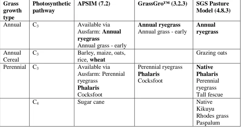
Economics and Sciences 2003). ...4 Table 1.2. The rate of leaf appearance relative to leaf position for different grass species, as reported in different studies. ... 16 Table 1.3. The rate of leaf elongation relative to leaf position for different grass species as reported in two studies. ... 17 Table 1.4. Grassland Fire Danger Classes, index, rate of spread and difficulty of suppression (after McArthur 1966) (Cheney and Gould 1995b). ... 30 Table 1.5. DST strategies for modelling components of leaf senescence. ... 42 Table 1.6. Grass species incorporated into common DST, listed by annual or perennial growth type. These are divided into use of the C3 or C4 photosynthetic
pathway, with cereals further separated. Species included in the following
experiments are highlighted by bold font. ... 48 Table 2.1. Identity and growth habit details for target species used in the study. . 55 Table 2.2. Pot layout across glasshouse bench where A, D, P and W indicate annual ryegrass, wallaby grass, phalaris and wheat respectively. ... 59 Table 2.3. Grass species measured at each field site. ... 60 Table 2.4. Location of field sites relative to nearest available SILO weather station (Bureau of Meteorology 2009). ... 65 Table 2.5. Observations and measurements recorded and leaf turnover rates. ... 66 Table 3.1. General description and management of South East SA pasture
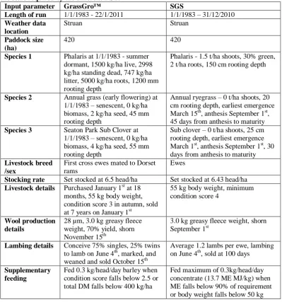
paddocks. ... 81 Table 3.2. Pasture, livestock and management starting parameters used for the phalaris pasture at Struan, SA in GrassGro™ and the SGS Pasture Model.
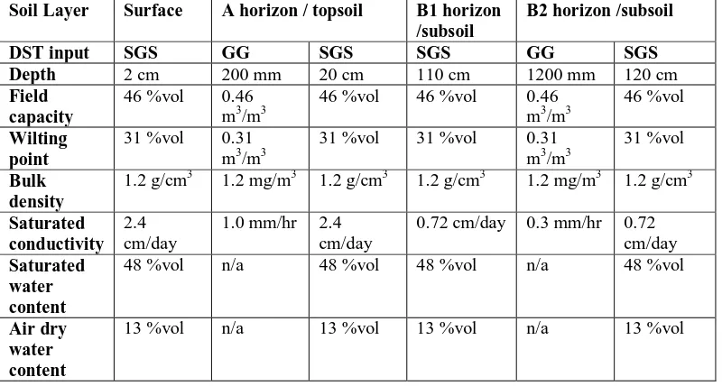
Parameters are given in the scale required by the different DST. ... 82 Table 3.3. Soil water module inputs for phalaris pasture at Struan, SA were derived from Principal Profile Form Ug5.11 from the Soil Atlas (Bureau of Rural Sciences (after CSIRO) 1991) in GrassGro™ (GG). These were used in the SGS Pasture Model, and extrapolated to the surface and B1 soil profiles which are not differentiated in GrassGro™. Parameters are given in the scale required by the different DST. ... 83 Table 3.4. Pasture, livestock and management starting parameters used for the annual ryegrass pasture at Struan, SA in GrassGro™ and the SGS Pasture Model. Parameters are given in the scale required by the different DST. ... 84 Table 3.5. Soil water module inputs for Struan, Naracoorte annual ryegrass
Table 5.1. Chi square statistics and probability, RMSD and Nash-Sutcliffe Model Efficiency Coefficient (E) and R2 derived from linear regression between LSR models fitted to LSR observations on which the models are based for each species. ... 126 Table 5.2. Chi square statistics and probability, RMSD and Nash-Sutcliffe Model Efficiency Coefficient (E) and R2 derived from linear regression between leaf length models fitted to leaf length observations on which the models are based for each species... 128 Table 5.3. Chi square statistics and probability, RMSD and Nash-Sutcliffe Model Efficiency Coefficient (E) and R2 derived from linear regression between LER models fitted to LER observations on which the models are based for each species. ... 130 Table 5.4. Leaf at which maximum LER occurs in each species. Standard errors and significance values refer to the comparisons between means and are given in brackets. Significant differences are indicated by different superscripts. ... 130 Table 5.5. Chi square statistics and probability, RMSD and Nash-Sutcliffe Model Efficiency Coefficient (E) and R2 derived from linear regression between LLS models fitted to LLS observations on which the models are based for each species. ... 131 Table 5.6. Chi square statistics and probability, RMSD and Nash-Sutcliffe Model Efficiency Coefficient (E) and R2 derived from linear regression between LAR models fitted to LAR observations on which the models are based for each species. ... 132 Table 5.7. Mean numbers of leaves and tillers. Standard errors and significance values refer to the comparisons between means and are given in brackets.
Significant differences are indicated by different superscripts. ... 133 Table 5.8. Summary of the shapes of models (stylised) for different leaf growth rates for four species, along with the leaf position at which rate maxima and minima occur. Note that for some rates, maximum and minimum values occur at multiple leaf positions, depending on the shape of the model. ... 134 Table 6.1. Number of samples of each species measured at field sites in the 2008-9 fire season. ... 142008-9 Table 6.2. Pot layout across glasshouse bench with timing of treatments indicated. A, D, P and W indicate annual ryegrass, wallaby grass, phalaris and wheat
Table 6.6. Chi square statistics and probability, RMSD and Nash-Sutcliffe Model Efficiency Coefficient (E) and R2 derived from cross validation techniques between the LSR models fitted to the LSR observations on which the models are based for each species when subjected to water stress in late spring. ... 156 Table 6.7. Chi square statistics and probability, RMSD and Nash-Sutcliffe Model Efficiency Coefficient (E) and R2 derived from linear regression between leaf length models fitted to leaf length observations on field-grown plants on which the models are based for each species. ... 158 Table 6.8. Chi square statistics and probability, RMSD and Nash-Sutcliffe Model Efficiency Coefficient (E) and R2 derived from cross validation techniques between the leaf length models fitted to the leaf length observations on which the models are based for each species when subjected to water stress in early spring. ... 159 Table 6.9. Chi square statistics and probability, RMSD and Nash-Sutcliffe Model Efficiency Coefficient (E) and R2 derived from cross validation techniques between the leaf length models fitted to the leaf length observations on which the models are based for each species when subjected to water stress in mid-spring. ... 160 Table 6.10. Chi square statistics and probability, RMSD and Nash-Sutcliffe Model Efficiency Coefficient (E) and R2 derived from cross validation
1 Introduction
Grass is a major vegetation component of Australian landscapes, and an important source of fuel for grassfires. Curing is the term used to describe
senescence and desiccation of grass material across the landscape, and is reported as the percentage of dead material in the sward (Anderson and Pearce 2003). Grass becomes increasingly flammable as the degree of curing increases. Fire management agencies require accurate and timely assessments of curing for planning activities such as prescribed burning, implementing fire prevention measures, and fire danger rating (Cheney and Sullivan 2008) for risk assessment purposes.
This thesis investigates the ability of pasture growth models currently
incorporated into commonly available agricultural decision support tools (DST) to improve the assessment of grass curing. Further, the thesis tests if a detailed understanding of the relationships between leaf growth rates can be applied to improve the accuracy of grass curing assessment through development of stand-alone models.
grass-dominated landscapes. An overview of the current methods of curing
measurement is given and the potential of agricultural plant growth DST for the assessment of grass curing is considered.
1.1 Temperate grasslands
In this thesis, the term “grasslands” describes grass-dominated landscapes, including cereal crops (Carter et al. 2003), as commonly used by fire management agencies. It does not adhere to strict ecological definitions (e.g.
Faber-Langendoen and Josse 2010). In Australian agricultural landscapes, grasslands comprise native and exotic grass and legume species with annual and perennial growth habits, along with a range of other herbs and forbs such as broad-leaf weeds.
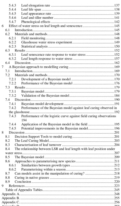
1.1.1 Australian climatic zones
Figure 1.1. Climatic regions of Australia (Munro et al. 2007).
1.1.2 Extent of grasslands in Australia
According to the Australian Bureau of Agricultural and Resource Economics (2003), 52% of the Australian continent is covered by native grasslands or
minimally modified pastures, with distribution of these grasslands differing markedly between the states (Table 1.1). Non-native grasslands comprise annual crops and both annual and perennial pastures and account for just 8% of the Australian land mass, and differ widely between the states (Table 1.1). The higher economic value of grasslands and their proximity to urban areas and other assets such as plantation forests give them high significance from a fire risk perspective.
Grasslands provide fine fuels to fires in the form of natural and improved (sown) pastures, and cereal and hay crops (Luke and McArthur 1978). Fire is used as a management tool in many grasslands, particularly those with high
1995a; Prober et al. 2007; Leonard et al. 2010; Murphy and Russell-Smith 2010). To date, research on curing has focused on improved pastures (ryegrass/clover mixtures) and cereal crops (Garvey 1989; Barber 1990; Martin 2009), largely ignoring native and naturalised species.
Table 1.1. Land area („000 sq km) of different Australian states and territories, and area („000 sq km) occupied by different grassland types with percentage of respective state, territory or continent land area given in brackets. Adapted from Integrated Vegetation Cover (Australian Bureau of Agricultural Resource Economics and Sciences 2003).
Total land area
Native grassland or minimally modified
pastures
Annual crops and highly modified
pastures
WA 2 327 1 599 (68.7) 186 (8.0)
SA 984 393 (39.9) 77 (7.8)
Vic 228 52 (23.0) 77 (33.7)
NSW 801 322 (40.2) 92 (11.5)
ACT 2 0.2 (8.0) 0.04 (1.5)
QLD 1 725 834 (48.4) 134 (7.8)
NT 1 348 698 (51.8) 2 (0.1)
TAS 68 4 (6.2) 12 (16.9)
Australia 7 483 3 903 (52.2) 579 (7.7)
1.1.3 Grassland types
Grasslands are categorized into different types describing the general arrangement of the grassland communities. Northern Australia is dominated by tropical grasslands, tussock grasslands and hummock grasslands, which were not included in this study. Temperate grasslands are generally comprised of native tussock grasslands, along with introduced pastures and cereal crops.
1.1.3.1
Native grasslands
The genera Austrodanthonia (H.P. Linder), Austrostipa (S.W.L. Jacobs & J. Everett), Bothriochloa (Kuntze), Chloris (Sw.), Enteropogon (Nees), Lomandra
throughout many regions of south eastern Australia. In Victoria, these tussock grassland communities occur on the plains of the Wimmera, Western Basalt, central Gippsland, and Northern districts. The South Eastern Highlands grassland ecological community stretches from Melbourne in Victoria to Bathurst in NSW. Other tussock grassland communities occur on the Liverpool and Moree plains, and the Riverina plain of NSW. In South Australia, tussock grasslands stretch from the Flinders Ranges to the mouth of the Murray River, while in Tasmania, tussock grasslands occur in the Northern Midlands, Northern Slopes, South East, Ben Lomond and Flinders Island bioregions (Carter et al. 2003). These grasses accumulate dead material in tussocks of about 30 cm in height, and they can accumulate large quantities of fuel in the absence of grazing or fire. Growth of other annual and perennial species between the tussocks contributes to the continuity of the fuel bed (Cheney and Sullivan 2008).
1.1.3.2
Introduced pastures
Grasslands are often termed “improved” where native species have largely been replaced by a mixture of introduced annual and perennial grasses and legumes, in an effort to increase the carrying capacity for livestock grazing
enterprises (Cheney and Sullivan 2008). Distribution of introduced pasture species is largely dependent on rainfall and altitude (Kemp and Dowling 1991).
In southern Australia, many of the introduced species have become naturalised, such as Phalaris aquatica L. (phalaris), Lolium rigidum Gaud.
(annual ryegrass), Trifolium subterraneum L. (subterranean clover) and Medicago
polymorpha L. (burr medic). The annualisation of many sown pastures has been
recognised in Victoria and New South Wales (Schroder et al. 1992; Kemp and Dowling 2000; Mason and Kay 2000; White et al. 2003; Friend et al. 2007; Mitchell 2008). In some cases, perennial native species have been able to exploit changes in soil fertility and grazing management (Virgona et al. 2002) and are increasingly being recognised as having a legitimate place in agriculture (Bellotti 2001; Dear et al. 2006; Islam et al. 2006; Mitchell 2008).
The fuel loads that result from pasture improvement are considered to be greater than those of native grasslands (Cheney and Sullivan 2008). Higher fuel loads and grass fires of greater intensity during summer are attributed to the shift from perennial to annual species, particularly cereals and weedy annual species across agricultural lands, and the suppression of fire as a land management tool (Chandler et al. 1983). This may be a reflection of management practices rather than biological composition. Improved pastures usually provide continuous fuel beds; however, these can be managed by grazing and mowing or slashing.
1.1.3.3
Crop lands
Broad acre cropping lands make up a small but highly valuable area of grass-dominated landscapes in Australia (3% of the land mass (Hutchinson 1992; Munro et al. 2007)). Wheat (Triticum aestivum L.) and barley (Hordeum vulgare
Accidental ignition of mature cereal crops by harvesting equipment is of concern to fire agencies (Miller 2008). Stubble remaining after harvest can also pose a fire risk and the increasing adoption of stubble retention practices will increase this risk. The presence of weeds or other grasses under the crop stubble can increase the fuel bed continuity (Cheney and Sullivan 2008).
1.2 Phenology of grasses
Growth and development of grasses are different, though related, concepts. Growth involves an expansion or enlargement of the plant structure, and in agriculture this translates to an increase in dry weight of leaf or grain matter. In contrast, development indicates a transition from one stage or phase to another, implying time units, but the interval between phases can also be measured in terms of temperature and photoperiod accumulation (Wilhelm and McMaster 1995; Campbell and Norman 1998). Plant growth occurs during development and may influence the final herbage or grain yield but the two processes should not be confused. Growth can cease under environmental stress but development will typically accelerate (Wilhelm and McMaster 1995). The study of plant
development as it relates to climate is known as phenology (Perry et al. 1987).
1.2.1 Grass development phenostages
industries is the reproductive phenostage and the associated production of seeds or grains.
Descriptions of grass plant development tend to focus on the development period of interest. Hence plant development guides for wheat (e.g. Figure 1.2) (Large 1954; Haun 1973; Zadoks et al. 1974) emphasise different phenostages to those for sown pasture grasses (Simon and Park 1983; Moore et al. 1991).
However, none adequately describe senescence of leaf material during vegetative, reproductive or subsequent phenostages. These phenostages are of particular importance in grass fuel and fire management and are described in general detail for grasses in the following sections.
Figure 1.2. Feekes scale of wheat development (Large 1954).
1.2.1.1
Vegetative phenostage
Plant development begins with the germination and emergence phenostages (Langer 1979). The following vegetative phenostage is characterised by the appearance and elongation of leaves, and the differentiation (but not elongation) of stem nodes (Moore and Moser 1995).
does not expand further, but does begin to photosynthesize. Leaf maturity is reached at the end of leaf cell division and sheath elongation and is signaled by the differentiation of the ligule. In general in sown pasture grass species, as the youngest leaf appears, the next oldest is rapidly growing, and the third oldest is reaching maturity (Langer 1979).
The vegetative phase may also involve tillering, where new shoots branch off from nodes or buds on the stem of the plant, and emerge through the lower leaf sheath. In grass species, tiller appearance usually begins after the first three leaves have appeared. Annual grasses produce tillers for a limited period, which may or may not flower (Langer 1979).
1.2.1.2
Reproductive phenostage
The transition from the vegetative to the reproductive phenostage can be triggered by a range of signals including temperature accumulation, photoperiod, vernalisation and leaf accumulation (McMaster and Wilhelm 1997). As
temperature increases in spring, green herbage production typically peaks. Species and cultivars may respond to different signals, and different threshold values at which these signals operate (McMaster and Wilhelm 1997). When the
reproductive phase begins, the stem elongates and no further leaf primordia are generated, capping the number of leaves, although they continue to appear until the leaf primordia are exhausted (Moore and Moser 1995). The bud primordia develop rapidly to form the inflorescence, which is enclosed in the sheath of the final or “flag” leaf, and is carried upwards by the elongating stem (Langer 1979).
Most grass species require a vegetative phase, when they are temporarily insensitive to the transitional signals such as photoperiod, before entering the reproductive phase. The vegetative phase may be quite short, as in the case of most annual grasses. Generally the reproductive phase is regarded as a point of no return, but some grasses can revert to vegetative proliferation if conditions, primarily photoperiod, are not conducive to completing seed set (Langer 1979).
1.2.1.3
Senescence phenostage in annual grasses
The lifecycle of grass growth and death in southern Australia follows the pattern of rainfall distribution. The annual and perennial grasses which use the C3
photosynthetic pathway display a seasonal life cycle involving death or dormancy to avoid the seasonal drought during summer in southern Australian. This
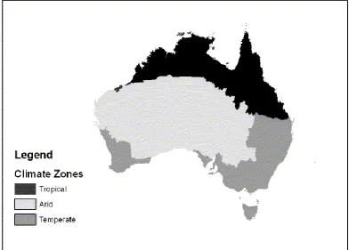
[image:34.595.72.469.451.655.2]senescence which is most obviously seen as chlorophyll loss (Nooden 2004) is accompanied by desiccation, and is termed “curing” in fire management circles.
Figure 1.3. Generalized diagram of annual pasture life cycle in a Mediterranean environment (Parrott 1964).
Annual plants go through “whole plant senescence” (Nooden et al. 2004) and die, leaving the dry standing residues associated with grass fuel. In a crop,
the dry plant material provides a standing “haystack” for livestock grazing. This general relationship is shown in Figure 1.3.
Senescence, which in grasses commences at the tip of the oldest leaf, is a development process which serves a number of purposes. It is an energy-demanding process (Thomas and Donnison 2000) in which accumulated and synthesised plant resources are actively mobilized (Buchanan-Wollaston and Morris 2000). In annual plants, senescence of vegetative tissue is the source of nitrogen and carbohydrate for the developing seed or grain (Frith and Dalling 1980). Once critical leaf area is reached, when the canopy intercepts 95% of incident light (Brougham 1960), older leaves begin to senesce and die (Moore and Moser 1995). Tillers die with the main stem. Ultimately, resources are salvaged by the plant to ensure ongoing survival through harsh environmental conditions in the form of seeds or dormant root stocks and crowns. Death is not always a consequence of senescence, and plants can die without senescing (Thomas and Donnison 2000).
1.2.1.4
Development variations of perennial grasses
Once the reproductive phase is reached, differences exist between perennial species in their subsequent rates of senescence. Tillers of Lolium perenne L. (perennial ryegrass) and Festuca arundinacea Schreb. (tall fescue) tend to be more resistant to death with only around 30% death rates in tillers which have flowered. In contrast, 90% of flowering tillers of Phleum pratense L. (timothy)
and Bromus willdenowii Kunth (prairie grass) will die (Valentine and Matthew
1999).
Perennial plants may grow for many years but herbaceous perennials exhibit annual growth followed by “top senescence” (Nooden 1988). This is a mechanism for escaping adverse weather conditions and in many parts of the world is
demonstrated by plants becoming dormant over the winter. In temperate climates like Australia however, perennial C3 grasses express a top senescence called
“summer dormancy” to avoid harsh summer conditions. Nutrient reserves (primarily carbon and nitrogen) are translocated from the aerial portions of the plant to the crown of the plant (Watson and Lu 2004). The grass develops a “resting organ” such as swollen stems or tubers with dormant buds at the time of floral initiation followed by top senescence with which to escape summer drought (Hoen 1968).
1.2.2 Curing
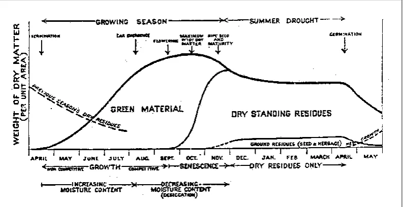
fire spread in grasslands. The assessment of curing in grasslands is in fact an assessment of the phenology of those grasslands.
Figure 1.4. Curing progress across Victoria 2007/8 (source: Country Fire Authority, Victoria)
This temporal and spatial variation is the result of variation in climate and species distribution. For instance, perennial plants tend to be distributed in higher rainfall areas which have longer growing seasons (Sanford et al. 2003) so that spring growth ends at different times between districts as illustrated by the curing map in Figure 1.4. Temporal variation in curing also occurs within districts. Perennials with extended growth period and later flowering time will display an extended curing pattern compared to the annual species growing in the same environment (Sanford et al. 2003).
To fully estimate the curing rates of grass plants, senescence from all triggers, whether they are phenological or environmental, must be accounted for to capture the transition from live to dead state and the accompanying changes in fuel
moisture.
1.2.3 Curing as a function of leaf growth processes
To determine curing in grass-dominated landscapes, knowledge of the change in proportion of the live and dead leaf pools in a sward over time is needed. The live pool is the culmination of leaf appearance and elongation to a fully expanded leaf length, for the duration of each leaf‟s life span, for all leaves in the sward. The dead leaf pool is determined by the onset and duration of senescence in each leaf in the sward.
Turnover of vegetative leaves in agriculturally-important perennial grasses and cereals has been well studied (e.g. Peacock 1976; Bircham and Hodgson 1983; Vine 1983; Chapman et al. 1984; Porter and Gawith 1999). However, often leaf rates have been reported on just a subset of leaves and cannot easily be
extrapolated to other species, regions and seasons (Bircham and Hodgson 1983; Grant et al. 1983). Linear measures of leaf turnover are not frequently available, but would overcome the need to harvest, and hence interrupt, the growth of the plant in order to determine the proportion of live and dead leaf pools over time. It is possible to convert linear measures to mass measures if leaf weight per unit length is known (Mazzanti et al. 1994; Hepp et al. 1996).
particularly temperature, but also photoperiod, water, nitrogen, salinity, light, CO2,
soil and seed factors (McMaster and Wilhelm 1995).
1.2.3.1
Leaf appearance rate
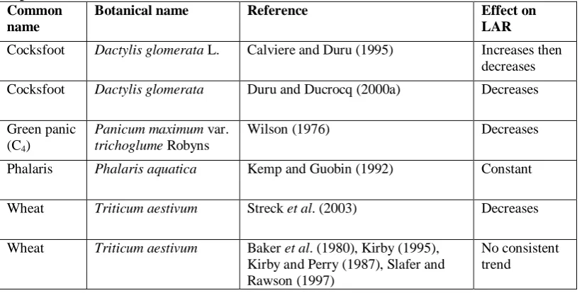
[image:40.595.66.477.448.655.2]Leaf turnover begins with the appearance of successive leaves. The time interval between leaves is described as “phyllochron”. The reciprocal of phyllochron is leaf appearance rate (LAR) which is the proportion of the leaf which has appeared in each time unit. Phyllochron is often assumed to be constant (McMaster et al. 1991; Rickman and Klepper 1995), however, there is evidence that the rate at which leaves appear may vary with increasing leaf position, but not always in the same direction (Table 1.2). Phyllochron varied between wheat tillers (Evers et al. 2005) and between years in several grass species (Frank and Bauer 1995), but was not reported for individual leaves.
Table 1.2. The rate of leaf appearance relative to leaf position for different grass species, as reported in different studies.
Common name
Botanical name Reference Effect on
LAR
Cocksfoot Dactylis glomerata L. Calviere and Duru (1995) Increases then decreases
Cocksfoot Dactylis glomerata Duru and Ducrocq (2000a) Decreases Green panic
(C4)
Panicum maximum var. trichoglume Robyns
Wilson (1976) Decreases
Phalaris Phalaris aquatica Kemp and Guobin (1992) Constant
Wheat Triticum aestivum Streck et al. (2003) Decreases
Wheat Triticum aestivum Baker et al. (1980), Kirby (1995), Kirby and Perry (1987), Slafer and Rawson (1997)
No consistent trend
1.2.3.2
Leaf elongation rate
length of leaf per unit of time or thermal time. Previous studies have reported the average leaf elongation rate (LER) of a number of leaves in kangaroo grass (Themeda triandra L.) (Wallace et al. 1985), or a subsample of leaves of perennial ryegrass and phalaris, expressed in terms of calendar time (Peacock 1975a; Kemp and Guobin 1992). However, the relationship between LER and leaf position differed not only between species, but also between years in the same species (Table 1.3).
Table 1.3. The rate of leaf elongation relative to leaf position for different grass species as reported in two studies.
Common name
Botanical name Reference Effect on LER
Green panic Panicum maximum var. trichoglume
Wilson (1976) Increases then decreases (non-linear)
Cocksfoot Dactylis glomerata Duru and Ducrocq (2000a)
Non-linear, linear and no response, varying between years
1.2.3.3
Leaf life span
Leaf life span (LLS) is usually defined as the period between leaf appearance and the onset of leaf senescence (Wilson 1976; Calviere and Duru 1995; Lemaire and Chapman 1996; Lemaire and Agnusdei 2000; Lemaire et al. 2009), but senescence has sometimes been included in LLS (Duru and Ducrocq 2000a; b). LLS has been documented as a single value for a range of species (Lemaire et al.
1.2.3.4
Leaf senescence rate
Senescent material is the dead portion of the leaf which is still in contact with the green component of the live leaf. Dead and senescent leaf material must be determined for curing to be modelled. Few studies have reported the proportion of dead material present in the sward. Wilman and Mares Martins (1977) captured the percentage of cured material every three days; however, their method of removing senescent leaf material directly from the green living material within the sward may have affected the subsequent senescence of the remaining leaf.
Thomas and Norris (1977) estimated the proportion of dead material present along the leaf length at monthly intervals. Their results may have been confounded, however, by decomposition of senescent material in the intervening period (Tainton 1974). The rate of senescence cannot be determined from such studies if the length of the leaves is unknown. Some studies have reported the number of leaves (Calviere and Duru 1995), or the length of tiller senescing per unit of thermal time (Duru and Ducrocq 2000a; b), rather than the rate of linear senescence in individual leaves in thermal time. Leaf senescence rate (LSR), expressed as length per day, increased linearly with leaf position in green panic, although a non-linear function could have also fitted the data (Wilson 1976). LSR increased with thermal time in cocksfoot (Duru and Ducrocq 2000a; b) but could not be related to leaf position.
1.2.3.5
Leaf length
plant (e.g. Lemaire and Agnusdei 2000). However, successive leaves do not necessarily develop in an identical fashion (Dale 1988), with leaf length being the characteristic to most obviously demonstrate differences between leaves. Leaf length increased with leaf position in perennial ryegrass, cocksfoot and green panic (Robson 1973; Wilson 1976; Duru and Ducrocq 2000a; b) and a small decrease in leaf length was observed in the penultimate or flag leaves of wheat and perennial grasses (Humphries and Wheeler 1963; Robson 1973; Hodgkinson and Quinn 1976; Wilson 1976; McMaster 1997; Evers et al. 2005).
Variation in leaf length might also explain variation in some leaf turnover rates. Evers et al. (2005) stated that there was little variation in the duration of elongation of leaves. If this is so, then shorter leaves at earlier leaf positions will have a slow LER and longer leaves at medium leaf positions will have a fast LER. It follows that the same might be true for appearance and senescence rates. If leaf length and other turnover characteristics vary between leaves, then it would make sense to present turnover rates in terms of leaf position, however this is not common.
1.2.3.6
Leaf numbers
time could alternatively be determined from LAR and the period of time elapsed (Streck et al. 2003).
Duru and Ducrocq (2000b) found that cocksfoot leaf numbers increased with both defoliation and nitrogen application. This was in contrast to Ong (1978), who found that the number of live leaves produced per perennial ryegrass tiller
remained relatively constant regardless of the level of nutrient treatment, but was reduced by shading. The number of live leaves could be used as a surrogate for LLS in determining the onset of senescence in each leaf, when old leaves were transferred into the dead pool (Vine 1983). The number of live leaves have been determined by multiplying LLS and LAR (Lemaire and Agnusdei 2000).
It is clear that leaf turnover is dependent on a number of genetic and
environmental components. Aspects of leaf turnover in early leaves have received some attention; however, there is a lack of detailed information on leaf turnover for the entire life cycle. Certainly, the literature is scant on leaf turnover dynamics, particularly the rate of leaf senescence, for annual and native species common in southern Australian grass-dominated landscapes. Also, the lack of consistency with which leaf turnover rates have been reported makes it difficult to use the existing information to develop a model to estimate grass curing.
1.3 Fire
In the simplest terms, fire requires fuel, oxygen and heat for ignition (Pyne et al. 1996; Cheney and Sullivan 2008). Energy previously stored in cellulosic material during photosynthesis is released as heat, along with light (Pyne et al.
1996).
evaporates any moisture present, and then begins to break down the material through pyrolysis (Cheney and Sullivan 2008). Ignition occurs at the transition point between endothermic and exothermic reactions, where fire can continue without a pilot heat source. Combustion is the third stage of burning, in which heat is released (Pyne et al. 1996). The products of thermal degradation include hydrocarbon gases which themselves can be ignited with sufficient temperature or an ignition source, to release heat. The additional heat can induce the process of drying, ignition and flaming in neighbouring material (Cheney and Sullivan 2008).
Flammability, or the ability or propensity for a fuel to burn, is the result of ignitability, sustainability, combustibility and consumability. Ignitability is defined as the time until ignition, after exposure to a heat source. Sustainability refers to the continuation of burning after the initial ignition or heat source is removed. Combustibility describes the rapidity or intensity of the burn (Anderson 1970; Dimitrakopoulos and Papaioannou 2001; White and Zipperer 2010). In addition, consumability is the proportion of the fuel consumed by combustion (White and Zipperer 2010). Of the four components of flammability, ignitability is the most important, for without it, the other components are irrelevant (White and Zipperer 2010).
1.3.1 Bushfire
(Flannigan et al. 2009). “Fine fuels” with a diameter of less than 6 mm are required for fires to establish. Fine fuels such as grass, leaves and twigs, are more easily ignited and are usually wholly consumed by fire, depending on moisture content. Heavy fuels such as logs require fine fuels to sustain ignition along the surface of the fuel (Luke and McArthur 1978; Bresnehan and Pyrke 1998).
Fire behaviour encompasses the aspects of flammability such as ignition, growth and spread of the fire (or sustainability) and its intensity, and hence is an important characteristic for fire management. Fire behaviour is determined by the surrounding environment, including the interactions between fuel, weather conditions such as temperature and wind speed, and topography (Packham et al.
1995). The fire itself can also influence the fire environment, which further affects fire behaviour (Pyne et al. 1996).
Fire sustainability is achieved through access to more fuel and oxygen. The speed at which a fire travels, known as rate of spread, is determined largely by wind speed (Cheney et al. 1993), the continuity and arrangement of the fuel bed, dead fuel moisture content and curing percentage of the fuel (Coleman and Sullivan 1996; Cheney et al. 1998), and slope of the terrain (Cheney and Sullivan 2008). Fuel load and height do not influence rate of spread in grass fuels (Cheney
et al. 1993), although both may influence the continuity of the fuel bed and flame height which impact on the difficulty of fire suppression. In grasslands, the continuity of the fuel bed is also influenced by the degree of disturbance through grazing or mowing.
the fire, relative to the wind direction and speed (Cheney and Sullivan 2008). Fire intensity and subsequently the hazard posed through reduction in opportunities for fire control, increase with fuel load (Gill et al. 1987) and impact on the ability to safely conduct planned burns or suppress wildfires.
1.3.2 Grassfire
Much of the research into wildfires globally has targeted forest fires (e.g. Stocks et al. 1988; Daniel and Ferguson 1989). Less research activity has been conducted into grassfires. Fires in grasslands and savannas make up 80-86% of all burned area globally (Flannigan et al. 2009). In Australia 72% of all fire damage is the result of grassfires (Gill et al. 1989; Cheney and Sullivan 2008). Grassfires have the potential to cause significant and catastrophic impacts on livestock, property and human life, and can provide an ignition source for fire in
neighbouring high-value forests (Marsden-Smedley and Catchpole 1995b) or peri-urban residential areas.
The flammability of grasses is derived from a number of characteristics. Grass swards have a high biomass of fine leaves, arranged so as to be highly aerated (Murphy and Russell-Smith 2010) which improves the access of oxygen and heat to the combustion process. Furthermore, grass swards often have a high proportion of cured leaves and the moisture content of cured grass can change rapidly (Dimitrakopoulos et al. 2010).
1.4 Fuel moisture content
content is used to determine the fire danger rating index which describes the degree to which fires will start, spread, cause damage and be difficult to suppress (Luke and McArthur 1978). Most fire danger rating systems use empirically determined relationships to ascertain fuel moisture content (Viney 1991).
The moisture content of fuels can be gravimetrically determined by weighing fresh, “wet” samples of the fuel in the field, then drying to a constant weight in an oven (usually 105°C for 24 hours), and reweighing to calculate moisture content (Barber 1990; Anderson et al. 2011). Moisture content is expressed as a
percentage of the oven-dry weight (ODW) of the fuel (Viney 1991; Aguado et al.
2007).
Grass fuel moisture content is affected by plant development and death. As pasture grasses mature, senesce and die or become dormant, moisture content falls rapidly from around 175% ODW (or 1.75 times ODW) at flowering and seed formation towards around 2% ODW (McArthur 1966; Parrott and Donald 1970b). Grasses are considered saturated at about 35% ODW, which is sufficient to allow self-extinguishment in many fuels (Cheney 1981).
1.4.1 Dead fuel moisture content
heat exchange (Hatton and Viney 1988) and both temperature and relative
humidity usually demonstrate clear diurnal fluctuations (Wilson 1958). Dead fuel moisture content can vary with aspect, altitude and shade, across a landscape (Catchpole 2002).
Typically, peaks of relative humidity and dead fuel moisture content coincide around dawn (Pook and Gill 1993). As temperature increases and relative
humidity decreases through the course of the day, the moisture content of dead grass moves towards equilibrium with relative humidity (McArthur 1966) but exhibits a lag in the gain and loss of water vapour, called hysteresis (Catchpole et al. 2001; Cheney and Sullivan 2008). The lag is variously reported as between one and four hours for grass fuels (Anderson 1990; Catchpole et al. 2001). For fine fuels, most of the variation in dead fuel moisture content occurs during the day (Hatton and Viney 1988). Relative humidity has been found to affect dead fuel moisture content in grasses more so than temperature (McArthur 1966), and Viney (1991) described the relationship as non-linear.
The moisture content of dead grass fuels can be quickly and reliably
1.4.2 Live fuel moisture content
The moisture content of growing plants is termed live fuel moisture content. Temperature and relative humidity influence live fuel moisture content through transpiration rates. Water is transpired from the leaves and replenished from soil water reserves (Tunstall 1988). Other environmental factors, particularly those that affect soil moisture content (rainfall, drought, and soil texture), also alter live plant moisture content through water availability.
Live fuel moisture content varies with plant part and the stage of growth (Hoen 1968; Luke and McArthur 1978). In lush, actively growing vegetation, the moisture content may be as high as several hundred percent of the dry weight of the plant (Parrott and Donald 1970a; Luke and McArthur 1978; Frame 1992). The senescence phenostage is associated with moisture loss, and at plant death, the moisture content reflects only the ambient moisture content of the environment. The live fuel moisture content of annual plants in mid-summer is influenced more by phenological stage than by environmental factors such as soil water availability (Dimitrakopoulos and Bemmerzouk 2003). Live fuel moisture responds more slowly than dead fuel moisture to environmental and atmospheric conditions and tends to remain higher than dead fuel moisture during spring and summer
(Catchpole 2002). It is a necessarily complex interaction between physical and biological processes, and as such, has received much less attention than dead fuel moisture content (Viegas et al. 2001).
1.4.3 The effect of fuel moisture content on grassfire behaviour
2007). Parrott and Donald (1970b) reported that fuel moisture content had a far greater effect on ignitability of annual pastures than did temperature and humidity. The drier the grass fuel, the easier it is to ignite (Catchpole et al. 2001; Catchpole 2002), and conversely, fuel with high moisture content is difficult to light without a sustained ignition source to drive the moisture out of the fuel (Dimitrakopoulos and Papaioannou 2001; Cheney and Sullivan 2008).
In comparison to dead fuel moisture, live moisture content has a marginal role in ignition (Chuvieco et al. 2004). Parrott and Donald (1970b) found that ignition could be achieved at least 40% of the time in grasses with 100% moisture content, and the success of ignition being sustained rose quickly after moisture content fell below 100% but varied between different annual grass species.
Although the fuel moisture of the live and dead components of the sward were not reported separately, with around 40% dry herbage in these grass fuel complexes (Parrott and Donald 1970b), it must be the relatively lower moisture content of the dead fuel component that enables ignition.
Once ignited, combustion is more likely to be sustained by dry fuels
(Catchpole et al. 2001; Catchpole 2002). When present, water vapour released by evaporation will tend to smother the fire by preventing oxygen from reaching the base of the fire. Water vapour also acts to reduce radiant heat, reducing the drying effect on fuel ahead of the firefront, and reducing fire intensity (Pompe and Vines 1966). Moisture contents of 18% to 35% have been found to be sufficient to extinguish ignition sources or prevent the continuation of the fire once alight (Catchpole 2002).
the dead fuel alone. Live moisture content must be taken into account because of the damping effect it has on the fire (Catchpole 2002), and therefore is also necessary in fire modelling (Chuvieco et al. 2004). Curing is used as an
alternative to live fuel moisture, to reflect the damping effect of live fuels on fire behaviour.
1.4.4 Uses of fuel moisture content in bushfire management
Fuel moisture content is a critical input to both the modelling of fire behaviour which is used by fire managers to plan controlled burns and fire suppression efforts, and in prediction of the fire danger rating used on a regional basis for community warning, preparedness and safety measures. Fire behaviour models and fire danger ratings have been developed for specific vegetation types (Cheney 1981; Packham et al. 1995).
1.4.4.1
Rate of fire spread
Fuel moisture and grass curing vary temporally and spatially, and this affects the rate of fire spread, the difficulty of suppression and the fire danger rating. The CSIRO Grassland Fire Spread Meter combines environmental variables with grassland variables of curing and condition (natural, grazed or “eaten out”) to estimate rate of fire spread across a continuous grassland. This gives an index of the difficulty of fire suppression in a “standard” 4 t/ha southern Australian pasture (Anonymous 2008a; Cheney and Sullivan 2008).
(Cheney et al. 1993; Cheney and Gould 1995a). The model may therefore not have captured the full effect of curing. Lower rates of spread than would be predicted for fully cured pastures would be expected where there is spatial variability in curing (Cheney and Gould 1995b). The increase in rate of spread as fuel moisture decreases is very sensitive to changes at very low moisture values (Cheney et al. 1998). Therefore, any inaccuracy in defining moisture content, particularly low dead fuel moisture content, will have a marked effect on the accuracy of rate of spread models (Trevitt 1988).
1.4.4.2
Fire danger ratings
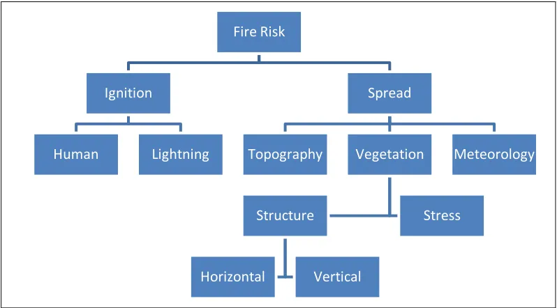
The terms “hazard”, “risk” and “danger” are often used interchangeably, but have specific meanings in fire management. Hazard refers to fuel factors such as quantity, arrangement, and flammability as well as the difficulty of fire
Figure 1.5. Components of fire risk (after Perestrello de Vasconcelos 1995).
Ratings of fire danger encapsulate the variables that represent severe fire weather and fuel flammability (Cheney and Gould 1995b). The fire danger ratings used in Australia use numerical indices and qualitative terms to represent the chance of a fire starting and spreading, its intensity and difficulty of suppression (McArthur 1966) (see Table 1.4). They are used by fire authorities to allocate resources for fire preparation, detection and suppression, and to provide public warnings to ensure safety and reduce the chance of ignition from land
[image:54.595.70.469.71.292.2]management or recreation activities (Cheney and Gould 1995b).
Table 1.4. Grassland Fire Danger Classes, index, rate of spread and difficulty of suppression (after McArthur 1966) (Cheney and Gould 1995b).
Fire Danger Class
Fire danger index (FDI)
Rate of spread at maximum FDI in class (km/hr)
Difficulty of suppression
Low 0 – 2.5 0.3 Low: headfire stopped by roads and tracks
Moderate 3 – 7.5 1.0 Moderate: headfire easily attacked with water
High 8 – 20 2.6 High: head attack generally successful
with water
Very high 20.5 – 50 6.4 Very high: head attack may fail except under favourable circumstances and back burning close to the head may be necessary
Extreme 50.5 – 100 12.8 Direct attack will generally fail – backburns difficult to hold because of blown embers. Flanks must be held at all costs.
Fire Risk
Ignition
Human Lightning
Spread
Topography Vegetation
Structure
Horizontal Vertical
Stress
Alan McArthur developed empirical models in the 1960s to represent fire danger for forest and grassland fuels which have been widely used in Australia, with occasional modifications. The Forest Fire Danger Index (FFDI) was developed from data drawn from 800 experimental fires in forests with 12 t/ha fuel loads (McArthur 1967). Weather variables were used to predict fine dead fuel moisture content using the McArthur FFDI (McArthur 1967). Moisture content was used to predict rate of fire spread, which in turn was assigned a relative fire danger rating (Cheney and Gould 1995b).
The McArthur Grassland Fire Danger Rating Index (McArthur 1966) and its successor, the Grassland Fire Danger Meter (Anonymous 2008c) used degree of curing between 70 and 100% as a surrogate for live fuel moisture content in establishing fire danger ratings for grasslands (Table 1.4). Degree of curing is also used in the Canadian Forest Fire Danger Rating System, to describe fire danger and spread in grasslands in Canada and New Zealand (Stocks et al. 1989;
McArthur Grassland Fire Danger Meter to predict fire danger at the regional level, and the rate of spread functions to be used at the site specific level (Cheney and Gould 1995b).
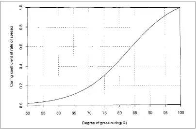
Fuel load influences the risk of fire occurring and the subsequent need for suppression. Fuel load was included in the fire danger rating in terms of grassland disturbance (heavily grazed through to undisturbed), to describe fuel bed
[image:56.595.70.475.318.585.2]continuity, even though it did not affect rate of spread. For instance, if a grassland is kept relatively short through grazing, there is little chance of a fire spreading, hence the fire danger is low (Cheney and Gould 1995b; Leonard et al. 2010).
Figure 1.6. The effect of degree of curing on the rate of fire spread (Cheney et al. 1998).
Fuel height is not included in either rate of spread equations, or the fire danger meter, but may have a small effect on the rate of spread. When taller, tussock-like grasses were grazed, the proportion of dead material remaining in the sward increased, as did the likelihood of sustainable burning (Leonard et al. 2010). Fuel height may also influence fire intensity and therefore the difficulty of
in the short term, while low dense fuels may be more easily approached, but be difficult to fully extinguish if allowed to smoulder (Cheney and Gould 1995b).
1.4.4.3
Planned fires
The use of planned fire is known variously as fuel reduction, controlled or prescribed burning, but the objectives of such burning may go well beyond fuel reduction. Planned burning is conducted in conditions that allow a fire to spread but to be controlled or self-extinguish (King et al. 2006; Higgins et al. 2011). As a fuel reduction strategy, planned burning reduces the amount and continuity of fine fuel, to reduce the number and intensity of subsequent unplanned fires, as well as the area burned. Fire suppression success in the landscape generally, and at the peri-urban interface, should subsequently increase (Bradstock et al. 1998; Fernandes and Botelho 2003; King et al. 2006; Cary et al. 2009; Higgins et al.
2011; Price and Bradstock 2011). Planned fire is also used to manipulate and maintain biodiversity in both forested and grassland ecosystems (Robertson 1985; Gill and Bradstock 1994; Marsden-Smedley and Catchpole 1995a; King et al.
2006).
behaviour of grassfires and the potential use of planned fire as a management tool in grasslands.
1.5 Curing as a surrogate for fuel moisture content in
grasses
The measurement of fuel moisture content is time consuming and labour intensive. Direct measures are often not readily available to fire agencies and operations in timeframes suitable for planned burns or in fighting wildfires. However, it is possible to use indirect measures if they are closely related to fuel moisture content and it makes sense to do so if these surrogates are accurate, timely, inexpensive and relatively easy to obtain (Purvis 1995).
In the case of grasslands, fuel moisture content is dependent on the
simultaneous moisture contents of both live and dead material within the sward. A relationship between fuel moisture content and curing values in grasslands has been developed (Parrott and Donald 1970b; Luke and McArthur 1978). Low curing percentage is associated with high fuel moisture while high curing percentage is associated with very low fuel moisture content (Figure 1.7).
Curing percentages less than 100 are a surrogate indicator for the moisture content of live fuel (Catchpole 2002). Accurate curing assessments are required for grassfire danger ratings to ensure the readiness of the general public and appropriate suppression forces when extreme fire weather is anticipated, and to calculate the rate of spread of fire in grasslands.