An Empirical Validation of the House Energy Rating
Software AccuRate for Residential Buildings in Cool
Temperate Climates of Australia
Detlev Geard, BA, Grad DipArch, MAEnvSt
A thesis submitted to the University of Tasmania in fulfilment of
the requirements for the degree of Doctor of Philosophy
Faculty of Science Engineering & Technology
School of Architecture and Design
University of Tasmania
Signed Statement
Declaration of Originality
This thesis contains no material which has been accepted for a degree or diploma by the University of any other Institution, except by way of background information and duly acknowledged in the thesis, and to be best of my knowledge and belief no material previously published or written by another person except where due acknowledgement is made in the text of the thesis, nor does the thesis contain any material that infringes copyrights.
Authority of Access
The authority of access statement should reflect any agreement which exists between the University and an external organization (such as a sponsor of the research) regarding the work. Examples of appropriate statements are:
Abstract
In 2003, the Building Code of Australia (BCA) introduced its first thermal performance requirements for residential buildings as a means to reduce Australia’s energy consumption and greenhouse gas emissions in the construction sector. This mandated a minimum energy performance rating of 4 stars for all new residential buildings. This requirement was increased to 5 stars in 2006 and to 6 stars in 2010. The introduction of the 4-star requirement had only a minor impact on construction practices and construction costs. However, the adjustment to 5 and 6-star ratings resulted in changes within the building industry, particularly on timber floor construction. The BCA's requirements for increased star ratings and energy efficiency resulted in concerns within the building industry, one of which was in relation to the accuracy of the House Energy Rating scheme's (HER) software "AccuRate" and its capability to model the building envelope and provide the star rating. AccuRate was developed gradually over a number of years by the CSIRO and was primarily used by building designers as a design tool. When the energy efficiency section was incorporated into the BCA as part of the building approval requirements, AccuRate was developed into a regulatory tool. Consequently, industry and government have recognized the need to validate this software empirically.
The University of Tasmania, in collaboration with Forest and Wood Products Australia, the Australian Government, and housing developer Wilson Homes, constructed three test houses in Kingston, Hobart for the purpose of validating AccuRate empirically for the cool temperate climate zones of Australia. The test houses were built to standard building practices, comprising: brick veneer walls, aluminum-framed windows and Colorbond steel roofing. Two houses have suspended timber floors and the third house has a concrete slab floor.
An extensive array of instruments and data loggers was installed to measure and document the thermal performance of the three houses. Comprehensive AccuRate simulations of the test houses were carried out, and hourly measured and simulated data were compared. The research presents the findings of the graphical and statistical analysis of the variation between the simulated and measured data from the three test houses.
Acknowledgements
I wish to express my appreciation to a number of people who have contributed in a substantial way to the writing of this PhD thesis.
Firstly I wish to thank my supervisors, Professor Roger Fay, Dr. Florence Soriano, Associate Professor Gregory Nolan and Dr. Alan Henderson, for their friendly support, advice and guidance for the duration of this project. Particular thanks go to Florence who always encouraged me with the words “you can do it”; especially at times when I doubted my intellect, she offered me the option to ring her for advice at any time, even at 2 a.m. in the mornings (I never did). Roger always found some nice words of encouragement throughout this long research process. I thank Greg for establishing this research project and all the assistance he provided, especially during the installation of the measuring equipment at the test houses.
My gratitude goes to Dr. Desmond FitzGerald and Chi-ho Yung, School of Mathematics and Physics, University of Tasmania, for the assistance and advice on writing the statistical analysis of this project.
I also thank Dr. Dong Chen at the CSIRO for the advice and guidance he so promptly provided about the development of the AccuRate software. At times, minutes after my e-mail questions to Dong, the response was already (thankfully) received.
Special thanks go also to Professor John Boland and Barbara Ridley who helped me with converting measured global solar radiation into diffuse solar radiation.
In addition I wish to thank for their help:
Dr. Heber Sugo from the University of Newcastle for showing me through the test cells in Newcastle and providing valuable advice on the selection of monitoring equipment for the test houses;
Dr Mark Luther for the establishment of air change rates for the test houses and his enormous enthusiasm for research in architectural science;
Max Fang and Vicky Kong who helped with the monumental task of data checking and cleaning the data;
Clark Liu who helped with the creation of the ‘on site’ climate data file;
Cong Huan who helped me with the installation of the sensors in the houses and his ability to squeeze into areas where I never could have gone.
Table of Contents
Signed Statement...i
Abstract... ii
Acknowledgements...iv
Table of Contents...vi
List of Tables ...ix
List of Figures... xiii
List of Acronyms ...xxi
Chapter 1: Introduction ...1
Chapter 2: Climate Change and the Construction Sector...7
2.1. History of the Climate Change Issue...7
2.2. Australia’s Greenhouse Gas Emission and Response to the Climate Change Issue...10
2.3. Australia’s Building Industry’s Strategy on the Reduction of Greenhouse Gas Emission...12
2.3.1. The Building Code of Australia Energy Efficiency Requirements...14
2.4. House Energy Rating Schemes in Other Developed Countries...18
2.5. Australia’s House Energy Rating Schemes ...22
2.5.1. History of Australia’s Nationwide House Energy Rating (NatHERS) Simulation Engine...23
2.5.2. AccuRate Rating Tool ...29
2.5.3. AccuRate Data Entry Process...30
2.5.4. The AccuRate Simulation Output...33
2.5.5. Current Australian Home Assessment Tools...36
2.6. Conclusion...37
Chapter 3: The Need for Validation of Building Thermal Simulation Programs ...39
3.1. Introduction ...39
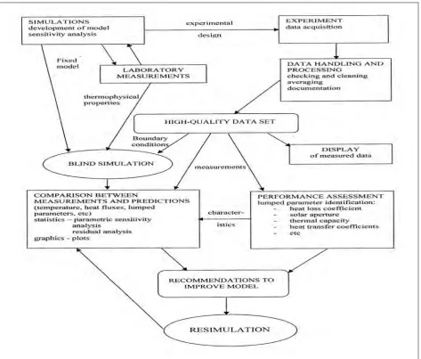
3.2. Validation Methodology...41
3.3. Data Collection Methodology ...43
3.4. Empirical Validation Methodology ...44
3.4.1. Definition of scope, type and nature of the physical and numerical experiment ...48
3.4.2. Implementation of the physical experiment on site ...49
3.4.3. Processing the measured data ...49
3.4.4. Performance of simulations ...49
3.4.5. Analysis of the results...49
3.4.6. Documentation of data set and validation work ...51
3.5. Empirical Validation Case Studies ...51
3.5.1. International Validation Research ...51
3.5.2. Australian Validation Research ...58
3.6. Conclusion...67
Chapter 4: Research Design and Empirical Validation Methods...68
4.1. Introduction ...68
4.2. The Physical Models ...69
4.2.1. Definition of AccuRate Output Temperature ...70
4.2.2. Developing an Environmental Measurement Profile...71
4.3. The Simulation Program ...74
4.3.1. As Built Construction Input Data ...75
4.3.2. Site Weather Input Data ...77
4.3.3. AccuRate’s Output Reports ...77
4.4. AccuRate Simulations ...79
4.4.1. Blind/Blind ...79
4.4.2. Blind/Climate ...79
4.4.3. As-Built/Blind ...79
4.4.4. As-Built/Climate...79
4.5. Methods of Analysing Validation Data ...80
4.5.1. Review of analytical methods and techniques ...80
4.5.2. Methods of Analysing Validation Data used in this Study...82
4.5.3. Correlation between measured and simulated temperatures...83
4.5.4. Residual Analysis ...84
4.6. Summary ...85
Chapter 5: Design and Construction of the Test Houses ...87
5.1. Introduction ...87
5.2. Determining the Star Rating Requirements of the Test Houses ...87
5.4. The Proposed Layout of the Floor Plan...92
5.5. The Floor Construction ...93
5.6. Exterior Wall Construction ...97
5.7. Aluminium Windows and Sliding Doors ...99
5.8. The Subfloor Construction of the Timber Floor Test Houses ...101
5.9. Ceiling and Roof Construction...102
5.10. Summary ...104
Chapter 6: Thermal Monitoring Equipment, Installation and Data Acquisition...107
6.1. Introduction ...107
6.2. Instrumentation Requirements...107
6.3. Sensor’s Location Plan and Profile ...109
6.4. The Monitoring Equipment ...112
6.4.1. The Data Logging System ...112
6.4.2. Sensors...116
6.4.3. Cabling and Wiring of Sensors to Data Logger...127
6.5. The Infiltration Test ...134
6.6. Data Management and Processing...136
6.6.1. DT 80 Data Logger and Local Area Network (LAN)...138
6.6.2. Method of Data Storage...139
6.6.3. Data Cleaning ...140
6.7. Summary ...143
Chapter 7: AccuRate Thermal Performance Simulations of the Test Houses...145
7.1. 1 Introduction ...145
7.2. AccuRate Simulation for the Purpose of Empirical Validation...146
7.3. AccuRate Simulation Inputs...147
7.3.1. Exposure and Ground Reflectance ...148
7.3.2. Construction Data ...149
7.3.3. Windows in Continuously Closed Position ...162
7.3.4. Zero Auxiliary Heating and Cooling Requirements ...162
7.4. Modification of AccuRate’s Scratch File ...162
7.4.1. Modification to Air Change Rates ...163
7.4.2. Window Framing Ratio ...165
7.5. The Climate Files ...167
7.5.1. AccuRate In-Built TMY Climate File ...167
7.5.2. Bureau of Meteorology (BOM) Climate File ...169
7.5.3. Site Measured Climate File ...170
7.5.4. Project Climate File ...171
7.6. AccuRate’s Output Data...173
7.6.1. General Output Data...174
7.6.2. Specific Output Data ...176
7.7. The Effects of Modified Construction Inputs and Site-Measured Climate File on AccuRate Simulation 177 7.8. Summary ...180
Chapter 8: Empirical Validation of AccuRate: Results & Discussion ...181
8.1. Introduction ...181
8.2. Selecting the Appropriate Temperature Measurements for Validation ...181
8.2.1. Comparison of Globe and Air Temperatures...181
8.2.2. Comparison of Air Temperatures at Different Height Levels ...186
8.2.3. Comparisons of Air Temperatures at Different Locations...187
8.2.4. Selection of Appropriate Temperature to Validate AccuRate ...191
8.3. Analysis of Empirical Validation Graphs...192
8.3.1. The Slab Floor House ...193
8.3.2. The 5-Star Timber Floor House...202
8.3.3. The 4-Star Timber Floor House...213
8.3.4. Comparison of Temperatures in various Zones of the Test Houses ...224
8.4. Empirical Validation Statistical Analysis...228
8.4.1. Introduction ...228
8.4.2. The Slab Floor House ...229
8.4.3. The 5-Star Timber Floor House...240
8.4.4. The 4-Star Timber Floor House...252
8.4.5. Comparison of the Three Test Houses...264
8.5. Summary of Statistical Analysis ...275
9.2. Conclusions ...281
9.3. Recommendation for further Research...284
References...288
Appendices...297
….Appendix 1: Photographic Documentation of the Installation of Measuring Equipment………...296
Appendix 2: Specification of Equipment………...299
Appendix 3: Simulated and Measured Temperatures for Bedroom 1, Bathroom and Garage for the Test Houses………..………317
Appendix 4: Statistical Scatterplotts, Residual Histograms and Fitted Temperature Values for other House Zones……….……...…..320
List of Tables
Table 2.1: Australia’s annual greenhouse gas emission between March 2008 and March 2009 ...11
Table 2.2: Maximum, minimum and mean temperatures in the free running test cells ...27
Table 2.3: AccuRate thermostat setting for climate zone 26, Hobart, Tasmania. ...31
Table 2.4: Time periods of heating and cooling for AccuRate. ...32
Table 3.1: Validation techniques...42
Table 3.2: Energy transport mechanism level ...44
Table 3.3: Comparison of measured and predicted heating energy for two week period ...53
Table 3.4: Comparison of measured and predicted air temperatures and heating demands for the NIST passive solar test facility ...55
Table 3.5: Maximum, minimum and mean temperatures in the free-running test cells ...57
Table 3.6: AccuRate default thermostat setting and new cooling thermostat settings ...61
Table 3.7: Percentage difference between monitored data and AccuRate simulation for the various cooling parameters ...61
Table 3.8: AccuRate’s suggested new thermostat setting for Adelaide ...62
Table 3.9: Percentage difference between monitored data and AccuRate simulation with three different settings based on a two year average data ...63
Table 4.1:: Environmental measured heights as specified by ASHRAE Standard 55 ...72
Table 4.2: Sample of AccuRate out-put data on simulated temperatures...78
Table 4.3: Degree of confirmation D and goodness-of-fit statistics...81
Table 5.1: Comparison of the star-rating fabric requirements for the three test houses...89
Table 5.2: Kingston climate data ...92
Table 6.1: AccuRate’s data input requirements ...108
Table 6.2: Sample of the DT 500 channel allocation spreadsheet for the 4 and 5-star timber floor house ...129
Table 6.3: Methods of storing data for the test houses...137
Table 6.4: Method of data cleaning of the test houses ...141
Table 7.1: Comparison of a standard AccuRate simulation and simulation for empirical validation ...146
Table 7.2: Parallel-path calculation method...151
Table 7.3: Isothermal-planes calculation method...152
Table 7.4: Calculating the wall framing factor for 12 individual wall elevations ...155
Table 7.5: Isothermal method to establish revised wall insulation...156
Table 7.6: Calculating the area and framing ratio of ceiling framing ...157
Table 7.7: Isothermal method to establish revised ceiling insulation...158
Table 7.8: Isothermal method to establish revised ceiling insulation...160
Table 7.9: Summary of reduction of ceiling insulation value due to framing ratio and installation of downlights for the test house ...161
Table 7.10: Calculation of required thickness, based on revised R-values for wall and ceiling insulation for the 4-star timber floor house...161
Table 7.12: AccuRate’s default values and measured values for air change per hour (value A) and
wind speed variables (B)...164
Table 7.13: Comparison of AccuRate’s in-built window framing ratios and measured window framing ratios for the houses ...166
Table 7.14: AccuRate climate file showing where coded information in each row is identified ...168
Table 7.15: Summary of AccuRate’s climate file data contents ...169
Table 7.16: Sample of the site climate data (EXCEL format)...171
Table 7.17: Summary of the site-project climate data file ...172
Table 7.18: Sample of AccuRate’s temperature files of hourly predicted temperatures ...176
Table 8.1: Comparison of air and globe temperatures in the living room of the slab floor house ...183
Table 8.2: Comparison of air and globe temperatures in bedroom 1 of the slab floor house...184
Table 8.3: Comparison of the centre and wall-mounted temperatures in the living room of the slab floor house ...188
Table 8.4: Comparison of wall-mounted and room centre-mounted temperature sensor in bedroom 1 of the slab floor house...190
Table 8.5: Comparison of measured and simulated temperatures in the living room of the slab floor house ...194
Table 8.6: Comparison of measured and simulated temperatures in bedroom 1 of the slab floor house ...196
Table 8.7: Comparison of measured and simulated temperatures in the hallway of the slab floor house...198
Table 8.8: Comparison of measured and simulated temperatures in the roof space of the slab floor house ...200
Table 8.9: Comparison of ranges, average minimum and average maximum measured and simulated temperatures of various zones in the slab floor house...202
Table 8.10: Comparison of measured and simulated temperatures in the living room of the 5-star timber floor house ...203
Table 8.11: Comparison of measured and simulated temperatures in the bedroom of the 5-star timber floor house ...205
Table 8.12: Comparison of measured and simulated temperatures in the hallway of the 5-star timber floor house ...207
Table 8.13: Comparison of measured and simulated temperatures in the roof space of the 5-star timber floor house ...209
Table 8.14: Comparison of measured and simulated temperatures in the subfloor of the 5-star timber floor house ...211
Table 8.15: Comparison of ranges, average minimum and average maximum measured and simulated temperatures of the 5-star timber floor house ...213
Table 8.16: Comparison of measured and simulated temperatures in the living room of the 4-star timber floor house ...214
Table 8.17: Comparison of measured and simulated temperatures in bedroom 1 of the 4-star timber floor house ...216
Table 8.19: Comparison of measured and simulated temperatures in the roof space of the 4-star timber
floor house ...220
Table 8.20: Comparison of measured and simulated temperatures in the subfloor of the 4-star timber
floor house ...222
Table 8.21: Comparison of ranges, average minimum and average maximum measured and simulated
temperatures of the 4-star timber floor house ...224
Table 8.22: Comparison of measured and simulated temperatures in various zones of the three test
houses...225
Table 8.23: Fitted values of simulated temperature at various measured temperatures for the living
room of the slab floor house ...231
Table 8.24: Fitted values of bedroom 2, hallway and roof space residuals at selected living room
residuals in the slab floor house ...233
Table 8.25: Fitted values of living room residuals at selected external temperatures of the slab floor
house ...235
Table 8.26: Fitted values of simulated temperature and corresponding residuals at various measured
temperatures for bedroom 1 in the slab floor house...236
Table 8.27: Fitted values of bedroom 2, hallway and roof space residuals at selected bedroom 1
residuals in the slab floor house ...238
Table 8.28: Fitted values of external temperature with bedroom 1 residuals in the slab floor house ...240
Table 8.29: Fitted values of simulated temperatures and at various measured temperatures in the living
room of the 5-star timber floor house ...242
Table 8.30: Fitted values of bedroom 1, hallway, roof space and subfloor residuals at selected living
room residuals in the 5-star timber floor house...244
Table 8.31: Fitted living room residuals at selected external temperatures in the 5-star timber floor
house ...246
Table 8.32: Fitted simulated temperatures and at various measured temperatures in bedroom 1 of the
5-star timber floor house ...247
Table 8.33: Fitted values of bedroom 2, hallway, roof space and subfloor residuals at selected
bedroom 1 residuals in the 5-star timber floor house...250
Table 8.34: Fitted values of bedroom 1 residuals at selected external air temperatures in the 5-star
timber floor house ...252
Table 8.35: Fitted values of simulated temperatures and corresponding residuals at various measured
temperatures in the living room in the 4-star timber floor house ...253
Table 8.36: Fitted values bedroom 2, hallway, roof space and subfloor residuals at selected living
room residuals in the 4-star timber floor house...256
Table 8.37: Fitted values of living room residuals at selected external temperatures in the 4-star timber
floor house ...258
Table 8.38: Fitted values of simulated temperatures and at various measured temperatures in bedroom
1 of the 4-star timber floor house...259
Table 8.39: Fitted values of bedroom 2, hallway, roof space and subfloor residuals at selected
Table 8.40: Fitted values of living room residuals at selected external air temperatures in bedroom 1 of
the 4-star timber floor house ...264
Table 8.41: Comparison of residuals of simulated temperatures at various measured temperatures in
the living room of the test houses ...266
Table 8.42: Comparison of residuals of fitted values of simulated temperatures at various measured
temperatures in bedroom 1 of the three test houses ...267
Table 8.43: Comparison of percentage time of over and under-prediction for the test houses ...268
Table 8.44: Comparison of actual maximum positive and negative residuals during the monitoring
period in the test houses ...268
Table 8.45: Fitted values of bedroom 2 residuals at selected living room residuals for the three test
houses...269
Table 8.46: Fitted values of roof space residuals at selected living room residuals for the three test
houses...270
Table 8.47: Fitted values of subfloor residuals at selected living room residuals for the 5-star and
4-star timber floor houses...271
Table 8.48: Fitted values of bedroom 2 residuals at selected bedroom 1 residuals for the three test
houses...271
Table 8.49: Fitted values of roof space residuals at selected bedroom 1 residuals for the three test
houses...272
Table 8.50: Fitted values subfloor residuals at selected bedroom 1 residuals for the timber floor houses ...272
Table 8.51: Fitted values of living room residuals at selected external air temperatures of the three test
houses...273
Table 8.52: Fitted values of bedroom 1 residuals at selected external air temperature of the three Test
Houses...274
Table 8.53: Calculated external air temperatures when the software changed prediction direction from
List of Figures
Figure 2.1: Mauna Loa Curve, concentration of CO2 in the atmosphere ... 7
Figure 2.2: Australia’s greenhouse gas emission March 1999 to March 2009 ... 10
Figure 2.3: Energy consumption and greenhouse gas emission by the building sector ... 13
Figure 2.4: Climate zone map ... 15
Figure 2.5: Climate zone map ... 15
Figure 2.6: British building energy rating certificate. ... 21
Figure 2.7: Comparison of monitored and simulated temperatures in a house in Melbourne and in Rockhampton. 25 Figure 2.8: Area correction factor for climate zone 26, Hobart ... 28
Figure 2.9: BESTEST comparison of low mass annual heating energy ... 29
Figure 2.10: BESTEST comparison of indoor temperature in a low mass building on a hot day with sudden increase in ventilation rate at 19:00 hours... 29
Figure 2.11: AccuRate heating and cooling energy requirements for the living room, climate zone 26, Hobart, Tasmania ... 34
Figure 2.12: AccuRate summary report. ... 35
Figure 2.13: Predicted AccuRate temperature profile for a brick veneer house in Kingston Tasmania. ... 36
Figure 3.1: Three level empirical validation methodology ... 46
Figure 3.2: Outline of the empirical, whole model validation methodology... 48
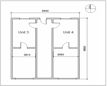
Figure 3.3: Floor plan of test buildings with two units ... 52
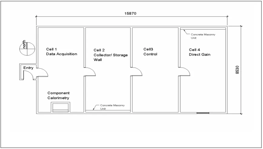
Figure 3.4: Floor plan of the NIST passive solar test building ... 54
Figure 3.5: Comparison of predicted and measured air temperature ... 56
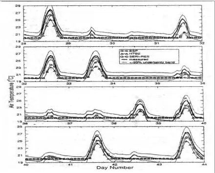
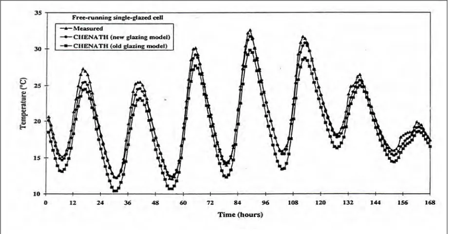
Figure 3.6: Measured and simulated temperatures for the free running single glazed test cell... 57
Figure 3.7: Comparison of monitored and simulated temperatures in the Broadmeadows and Rockhampton houses... 58
Figure 3.8: Floor plan of the mudbrick house. The rectangles indicate the positions of heaters, the diamonds the comfort carts and the circles the B&K meter ... 59
Figure 3.9: Final comparison of temperatures predicted by AccuRate with measured air temperatures. ... 60
Figure 3.10: Monitored and AccuRate monthly energy use prediction for the different cooling parameters ... 62
Figure 3.11: Monthly energy use from monitored data and AccuRate predictions, with new and old default settings ... 63
Figure 3.12: Test cell with un-enclosed platform timber floor ... 64
Figure 3.13: Test cell with enclosed platform timber floor... 64
Figure 3.14: Temperature sensor installation at the test cells in Launceston ... 65
Figure 3.15: Simulated and measured indoor temperature in test cell 2 (enclosed timber floor) during a cold week. ... 66
Figure 3.16: Simulated and measured indoor temperature in test cell 3 (concrete slab-on-ground floor) during a cold week. ... 66
Figure 3.18: Simulated and measured indoor temperature in test cell 3 (slab on ground floor) during a warm
week. ... 66
Figure 4.1: Schematic diagram of the empirical validation method used in this study ... 68
Figure 4.2: PASSLINK test building ... 72
Figure 4.3: Interior of PASLINK test building ... 72
Figure 4.4: Three test cells at University of Newcastle... 73
Figure 4.5: Location of thermocouples and heat flux sensors within the test cells ... 73
Figure 4.6: Internal view showing the heat flux sensor at the window, air temperature sensors at the pole, DT 600 Data logger and the thermocouple isothermal box... 73
Figure 4.7: Shielded thermocouple installation at the sliding door ... 73
Figure 4.8: Horizontal environmental measurement profile of Launceston test cell with a concrete slab on ground floor ... 74
Figure 4.9: Outdoor, simulated and measured temperatures in test cell 1 during a cold week ... 83
Figure 5.1: Top view of the building site toward Auburn Road ... 90
Figure 5.2: View up the building site from Auburn Road... 90
Figure 5.3: The building layout at Auburn Road Kingston... 91
Figure 5.4: Aerial view of the completed housing development with the test houses on the left-hand side of the driveway... 91
Figure 5.5: Floor plan layout of the test houses ... 93
Figure 5.6: Timber bearers and floor joist construction detail ... 94
Figure 5.7: Timber particleboard platform and enclosed subfloor construction detail ... 94
Figure 5.8: Enclosed timber platform construction detail at the 4-and 5-star test houses ... 95
Figure 5.9: Section drawing of the timber floored test house ... 95
Figure 5.10: Fill preparations for the slab house before pouring of the concrete floor. ... 96
Figure 5.11: The concrete slab floor after pouring of concrete floor ... 96
Figure 5.12: Construction detail of the slab floor test house depicting the perimeter wall detail ... 96
Figure 5.13: Section detail of the brick veneer wall at the test houses... 97
Figure 5.14: Taping of sarking to the damp-proof course sheeting... 98
Figure 5.15: Installation of the sarking. ... 98
Figure 5.16: Installation of the wall insulation... 98
Figure 5.17: Shoddy installation of wall insulation ... 98
Figure 5.18: BCA eaves construction detail with an open cavity to the roof space ... 99
Figure 5.19: Awning window frame detail of the test house with concrete slab... 100
Figure 5.20: Awning window frame detail of the test house with concrete slab... 100
Figure 5.21: Elevations of the test houses and placement of windows and sliding doors... 100
Figure 5.22: Subfloor of the timber floor houses ... 101
Figure 5.23: Interior view of the ventilation grille from the subfloor ... 101
Figure 5.24: Ventilation grille installed to the brick perimeter foundation wall ... 102
Figure 5.25: Ventilation grille detail of the rendered perimeter foundation wall... 102
Figure 5.26: Installation of timber roof trusses onto the exterior stud wall ... 102
Figure 5.27: Interior view to the roof trusses and reflective sarking... 102
Figure 5.29: Internal view of a recessed ceiling downlight... 104
Figure 5.30: Installation of ceiling insulation between ceiling joists ... 104
Figure 5.31: Installation of the downlight guards ... 104
Figure 5.32: Installation of the downlight fittings... 104
Figure 5.33: The completed 5-star timber house... 105
Figure 5.34: Inside view of the 5-star timber house... 105
Figure 5.35: The slab house as seen from Auburn Road, Kingston ... 105
Figure 5.36: The housing development at Auburn Rd, Kingston, with the test houses at the right hand site of driveway... 105
Figure 6.1: Location of poles with sensors attached at various heights levels ... 109
Figure 6.2: Sensors attached to pole at 600mm, 1200mm and 180mm above floor level... 110
Figure 6.3: Globe thermometer (A) and dry bulb air temperature sensor attached to the inside of the plastic casing (B) ... 110
Figure 6.4: Location of permanent temperature sensors attached to the walls at a height of 1.2m from floor level110 Figure 6.5: Vertical profile of measurements for the 4-and 5-star timber floor houses ... 111
Figure 6.6: Vertical profile of environmental measurements for the slab house... 111
Figure 6.7: Horizontal profile of measurements through the north and south side of the brick veneer wall section of houses ... 112
Figure 6.8: Connection of sensors to the data logger ... 114
Figure 6.9: Data logger DT 500 and channel expansion module installed in the metal box ... 114
Figure 6.10: Installation of the data logger external metal box under the timber decking ... 114
Figure 6.11: Sample of DT 500 logger programming... 116
Figure 6.12: AD 592 CN temperature sensors attached to wall plate at the wall... 117
Figure 6.13: Numerous AD592 CN temperature sensors with bell wires attached for preliminary measuring of the air temperature at the centre of the room. ... 117
Figure 6.14: Air temperature sensor attachment to timber pole at the centre of rooms ... 118
Figure 6.15: Timber pole with temperature sensors located at different height levels... 118
Figure 6.16: Temperature sensor fixed inside a plastic pipe, covered by reflective foil ... 118
Figure 6.17: Wall-mounted dry bulb air temperature sensor and thermostat cover plate ... 119
Figure 6.18: Wall-mounted air temperature sensor located in a thermostat housing ... 119
Figure 6.19: Wall-mounted temperature sensor with bell wire connection... 119
Figure 6.20: Temperature sensor fixed to pole at mid-subfloor space hardly visible ... 120
Figure 6.21: Temperature sensor fixed to pole at mid-subfloor space ... 120
Figure 6.22: Temperature sensors attached to the outside of roof... 121
Figure 6.23: Temperature sensors taped onto inside of roof sarking with reflective silver adhesive tape ... 121
Figure 6.24: Temperature sensor attached to the inside of ceiling before being plastered over... 121
Figure 6.25: Temperature sensor attached to the underside of the timber floor (glued and taped) ... 121
Figure 6.26: Installing the sensor to the interior side of the slab floor... 122
Figure 6.27: Installing the waterproof temperature sensor housing and wire connection for the temperature sensor 1m below ground surface of the slab house ... 122
Figure 6.28: Sensor attached to the inside of the plasterboard wall ... 123
Figure 6.30: Sensor attached to the outside of the sarking... 123
Figure 6.31: Sensor before being attached to the inside the of brick wall... 123
Figure 6.32: Sensor attached to the inside of the brick wall with red cloth tape... 123
Figure 6.33: Sensor attached to the inside of the brick wall with red cloth tape... 123
Figure 6.34: Inserting the air temperature sensor into the globe thermometer... 124
Figure 6.35: Globe thermometer measuring environmental temperatures ... 124
Figure 6.36: Humidity transmitter installed in the ceiling space... 125
Figure 6.37: Humidity transmitter located in the subfloor space ... 125
Figure 6.38: SolData 80SPC pyranometer fixed to four external walls of test houses measuring solar radiation on the walls ... 126
Figure 6.39: SolData 80SPC pyranometer installed on the roof as part of the weather station measuring global and north vertical solar radiation... 126
Figure 6.40: Site Weather Station installed on top of the roof of the slab floor house ... 127
Figure 6.41: DT 80 indicating air temperature at the weather station ... 127
Figure 6.42: Wiring diagram for the cabling and wiring connection between the data logger and the individual sensors installed in the houses ... 128
Figure 6.43: Temperature sensors attached to bell wire... 130
Figure 6.44: Installation of data cables connecting sensors to Data Logger ... 130
Figure 6.45: Krone connectors connecting data cables to sensors via bell wires... 130
Figure 6.46: Krone connectors fixed to the floor joist connecting data cable to bell wire... 130
Figure 6.47: Data cable connecting to data logger with RJ 45 plugs ... 130
Figure 6.48: Data cable and RJ 45 plugs connection to the data logger’s RJ 45 terminal ... 130
Figure 6.49: Step 1. Installation and testing of data cable and plug connection ... 133
Figure 6.50: Step 2. Attaching second RJ 45 plug to data cable ... 133
Figure 6.51: Step 3. Connecting the RJ 45 plug into the Krone connector ... 133
Figure 6.52: Step 4. Connecting the sensor feeder cable into the Krone connector block ... 133
Figure 6.53: Connecting and checking sensor feeder cable on site... 134
Figure 6.54: Checking cable connection and data logger’s zero value readouts... 134
Figure 6.55: Comfort cart measurement equipment... 135
Figure 6.56: Tracer gas computer graph ... 135
Figure 6.57: Interior view of the blower door equipment installed at the test houses... 135
Figure 6.58: View of the pressurisation fan of the blower door equipment ... 135
Figure 6.59: Manual downloading of data from the data logger to the computer ... 136
Figure 6.60: Downloading data with the De Transfer program to the computer... 136
Figure 6.61: DT 80 data logger installation ... 137
Figure 6.62: Schematic diagram of the Local Area Network connection to the University’s server ... 138
Figure 6.63: Inserting the cable into conduit for the DT 500 to DT 80 cable connection... 139
Figure 6.64: Installing the cabling connection between the DT 500 and DT 80... 139
Figure 6.65: Downloading weather data from the DT 80 ... 139
Figure 6.67: Solar radiation received at the eastern wall of the 5-star timber floor house on 18.7.2007 between
8a.m. and 1p.m... 143
Figure 7.1: Typical brick veneer wall with 90mm stud framing spaced at 450mm centres ... 150
Figure 7.2: Timber framing of the test house showing the ratio of studwork as part of the whole wall ... 150
Figure 7.3: Corner detail of the framing stage of the test house ... 153
Figure 7.4: Framing stage of the test house ... 153
Figure 7.5: Completed wall framing stage of the test house ... 153
Figure 7.6: Framing stage of the concrete slab test house... 153
Figure 7.7: Elevation of external views of wall framing of the test houses ... 154
Figure 7.8: Diagram of the ceiling framing layout... 157
Figure 7.9: Diagram showing an uninsulated area around recessed light fittings in the test houses, as installed by the electrician to AS 3600 ... 159
Figure 7.10: Thermal image of the recessed downlight and gap of insulation around the light fitting ... 159
Figure 7.11: Photo of recessed downlight fittings installed in the test houses ... 159
Figure 7.12: Original AccuRate’s scratch file data for values A and B ... 164
Figure 7.13: Modified wind speed data for the kitchen/dining area of the slab floor house ... 165
Figure 7.14: Summary of air change rates in the roof space and kitchen/dining/living area for various wind speeds for the houses. (house 1 represents the slab floor house, house 2 the 5-star timber house and house 3 the 4-star timber house) ... 165
Figure 7.15: Window frame detail for the bedroom window at the 5-star timber floor house... 166
Figure 7.16: Close up of window framing detail... 166
Figure 7.17: Temperature profile comparison betwee site-measured air temperature and the BOM data, measured at the Ellerslie Road station, Hobart ... 173
Figure 7.18: Summary of the star rating report for the slab floor house ... 175
Figure 7.19: AccuRate’s general output data, predicted temperature profile for a typical cold winter period in the slab house’s kitchen/dining/living area, bedroom 1 and external temperature ... 176
Figure 7.20: AccuRate simulation comparison between as designed and as built condition of the slab house ... 177
Figure 7.21: Temperature comparison between AccuRate in-built climate data (TMY) and site measured climate data... 178
Figure 7.22: Global solar radiation data comparison between AccuRate climate data (TMY) and site-measured climate data ... 179
Figure 7.23: AccuRate simulation based on AccuRate’s TMY climate and measured site climate data ... 180
Figure 8.1: Comparison of air and globe temperature in the living room of the slab floor house... 182
Figure 8.2: Comparison of daily maximum and minimum temperatures of globe and air temperature in the living room of the slab floor house ... 183
Figure 8.3: Comparison of air and globe temperatures in bedroom 1 of the slab floor house ... 184
Figure 8.4: Comparison of daily maximum and minimum temperature of globe and air temperature in bedroom 1 of the slab floor house... 185
Figure 8.5: Comparison of air temperature at different height levels in the living room of the slab floor house ... 186
Figure 8.6: Comparison of air temperature at different height levels in bedroom room 1 of the slab house ... 187
Figure 8.8: Daily temperature difference between wall and centre-mounted sensors in the living room of the slab
floor house ... 189
Figure 8.9: Temperature comparison of centre-mounted and wall-mounted sensors in bedroom 1 of the slab
floor house ... 190
Figure 8.10: Daily temperature difference between wall and centre-mounted sensors in bedroom 1 of the slab
floor house ... 191
Figure 8.11: Comparison of simulated and measured temperature in the living room of the slab floor house ... 194
Figure 8.12: Comparison of simulated and measured maximum and minimum daily temperatures in the living
room of the slab floor house ... 195
Figure 8.13: Comparison of simulated and measured temperatures in bedroom 1 of the slab floor house... 196
Figure 8.14: Comparison of simulated and measured maximum and minimum daily temperatures in bedroom 1
of the slab floor house... 197
Figure 8.15: Comparison of simulated and measured temperatures in the hallway of the slab floor house ... 198
Figure 8.16: Comparison of simulated and measured maximum and minimum daily temperatures in the hallway
of the slab floor house... 199
Figure 8.17: Comparison of simulated and measured temperatures in the roof space of the slab floor house... 200
Figure 8.18: Comparison of simulated and measured daily maximum and minimum temperatures in the roof
space or the slab floor house ... 201
Figure 8.19: Comparison of simulated and measured temperatures in the living room of the 5-star timber floor
house ... 203
Figure 8.20: Comparison of simulated and measured daily minimum and maximum temperatures in the living
room of the 5-star timber floor house ... 204
Figure 8.21: Comparison between simulated and measured temperatures in bedroom 1 of the 5-star timber floor
house ... 205
Figure 8.22: Comparison of simulated and measured daily maximum and minimum temperatures in bedroom 1
of the 5-star timber floor house... 206
Figure 8.23: Comparison of simulated and measured temperatures in the hallway of the 5-star timber floor house207
Figure 8.24: Comparison of simulated and measured daily maximum and minimum temperatures in the hallway
of the 5-star timber floor house... 208
Figure 8.25: Comparison of simulated and measured temperatures in the roof space of the 5-star timber floor
house ... 209
Figure 8.26: Comparison of simulated and measured daily maximum and minimum temperatures in the roof
space... 210
Figure 8.27: Comparison of simulated and measured temperatures in the subfloor of the 5-star timber floor
house ... 211
Figure 8.28: Comparison of simulated and measured daily maximum and minimum temperatures in the subfloor212
Figure 8.29: Comparison of simulated and measured temperatures in the living room of the 4-star timber floor
house ... 214
Figure 8.30: Comparison of simulated and measured daily maximum and minimum temperatures in the living
room of the 4-star timber floor house ... 215
Figure 8.32: Comparison of simulated and measured maximum and minimum daily temperatures in bedroom 1
of the 4-star timber floor house... 217
Figure 8.33: Comparison of simulated and measured temperatures in the hallway of the 4-star timber floor house218 Figure 8.34: Comparison of simulated and measured daily maximum and minimum temperatures in the hallway of the 4-star timber floor house... 219
Figure 8.35: Comparison of simulated and measured temperatures in the roof space of the 4-star timber floor house ... 220
Figure 8.36: Comparison of simulated and measured daily maximum and minimum temperatures in the roof space of the 4-star timber floor house ... 221
Figure 8.37: Comparison of simulated and measured temperatures in the subfloor of the 4-star timber floor house ... 222
Figure 8.38: Comparison of simulated and measured daily maximum and minimum temperatures in the subfloor of the 4-star timber floor house... 223
Figure 8.39: Scatterplot of simulated versus measured temperatures for the living room of the slab floor house.. 230
Figure 8.40: Distribution of residuals for the living room of the slab floor house... 231
Figure 8.41: Scatterplot of living room and bedroom 2 residuals of the slab floor house... 232
Figure 8.42: Scatterplot of living room and hallway residuals of the slab floor house ... 232
Figure 8.43: Scatterplot of living room and roof space residuals of the slab floor house ... 232
Figure 8.44: Scatterplot of living room residuals and external air temperature of the slab floor house... 234
Figure 8.45: Scatterplot of living room residuals and global solar radiation of the slab floor house... 234
Figure 8.46: Scatterplot of living room residuals and wind speed of the slab floor house... 234
Figure 8.47: Scatterplot of living room residuals and wind direction of the slab floor house... 234
Figure 8.48: Scatterplot of simulated temperature versus measured temperature for bedroom 1 of the slab floor house ... 235
Figure 8.49: Distribution of residuals for bedroom 1 of the slab floor house ... 236
Figure 8.50: Scatterplot of bedroom 1 and bedroom 2 residuals of the slab floor house ... 237
Figure 8.51: Scatterplot of bedroom 1 and hallway residuals of the slab floor house... 237
Figure 8.52: Correlation of bedroom 1 and roof space residuals of the slab floor house... 237
Figure 8.53: Scatterplot of bedroom 1 residuals and external air temperature of the slab floor house ... 239
Figure 8.54: Scatterplot of bedroom 1 residuals and global solar radiation of the slab floor house ... 239
Figure 8.55: Scatterplot of bedroom 1 residuals and wind speed of the slab floor house ... 239
Figure 8.56: Scatterplot of bedroom 1 residuals and wind direction of the slab floor house ... 239
Figure 8.57: Scatterplot of simulated and measured temperature for the living room of the 5-star timber floor house ... 241
Figure 8.58: Distribution of residuals for the living room of the 5-star timber floor house... 242
Figure 8.59: Scatterplot of the living room and bedroom 2 residuals of the 5-star timber floor house... 243
Figure 8.60: Scatterplot of the living room and hallway residuals of the 5-star timber floor house ... 243
Figure 8.61: Scatterplot of the living room and roof space residuals of the 5-star timber floor house ... 243
Figure 8.62: Scatterplot of the living room and subfloor residuals of the 5-star timber floor house... 243
Figure 8.63: Scatterplot of living room residuals and external air temperature of the 5-star timber floor house.... 245
Figure 8.64: Scatterplot of living room residuals and global solar radiation of the 5-star timber floor house... 245
Figure 8.66: Scatterplot of living room residuals and wind direction of the 5-star timber floor house... 245
Figure 8.67: Scatterplot of simulated and measured temperatures for bedroom 1 of the 5-star timber floor house 247 Figure 8.68: Distribution of residuals for bedroom 1 of the 5-star timber floor house ... 248
Figure 8.69: Scatterplot of bedroom 1 and bedroom 2 residuals of the 5-star timber floor house ... 249
Figure 8.70: Scatterplot of bedroom 1 and hallway residuals of the 5-star timber floor house... 249
Figure 8.71: Scatterplot of bedroom 1 and roof space residuals of the 5-star timber floor house... 249
Figure 8.72: Scatterplot of bedroom 1 and subfloor residuals of the 5-star timber floor house... 249
Figure 8.73: Scatterplot of bedroom 1 residuals and external air temperature of the 5-star timber floor house ... 251
Figure 8.74: Scatterplot of bedroom 1 residuals and global solar radiation of the 5-star timber floor house ... 251
Figure 8.75: Scatterplot of bedroom 1 residuals and wind speed of the 5-star timber floor house ... 251
Figure 8.76: Scatterplot of bedroom 1 residuals and wind direction of the 5-star timber floor house ... 251
Figure 8.77: Scatterplot of simulated and measured temperatures for the living room of the 4-star timber floor house ... 253
Figure 8.78: Distributions of residuals for the living room of the 4-star timber floor house ... 254
Figure 8.79: Scatterplot of the living room and bedroom 2 residuals of the 4-star timber floor house... 255
Figure 8.80: Scatterplot of the living room and hallway residuals of the 4-star timber floor house ... 255
Figure 8.81: Scatterplot of the living room and roof space residuals of the 4-star timber floor house ... 255
Figure 8.82: Scatterplot of the living room and subfloor residuals of the 4-star timber floor house... 255
Figure 8.83: Scatterplot of living room residuals and external air temperature of the 4-star timber floor house.... 257
Figure 8.84: Scatterplot of living room residuals and global solar radiation of the 4-star timber floor house... 257
Figure 8.85: Scatterplot of living room residuals and wind speed of the 4-star timber floor house... 257
Figure 8.86: Scatterplot of living room residuals and wind direction of the 4-star timber floor house... 257
Figure 8.87: Scatterplot of simulated and measured temperature for bedroom 1 of the 4-star timber floor house . 259 Figure 8.88: Distribution of residuals in bedroom 1 of the 4-star timber house………..…260
Figure 8.89: Scatterplot of bedroom 1 and bedroom 2 residuals of the 4-star timber floor house ... 261
Figure 8.90: Scatterplot of bedroom 1 and hallway residuals of the 4-star timber floor house... 261
Figure 8.91: Scatterplot of bedroom 1 and roof space residuals of the 4-star timber floor house... 261
Figure 8.92: Scatterplot of bedroom 1 and subfloor residuals of the 4-star timber floor house... 261
Figure 8.93: Scatterplot of bedroom 1 residuals and external air temperature of the 4-star timber floor house ... 263
Figure 8.94: Scatterplot of bedroom 1 residuals and global solar radiation of the 4-star timber floor house ... 263
Figure 8.95: Scatterplot of bedroom 1 residuals and wind speed of the 4-star timber floor house ... 263
Figure 8.96: Scatterplot of bedroom 1 residuals and wind direction of the 4-star timber floor house ... 263
Figure 8.97: Scatterplot of simulated and measured temperatures for the living room of the slab floor house ... 265
Figure 8.98: Scatterplot of simulated and measured temperatures for bedroom 1 of the slab floor house ... 265
Figure 8.99: Scatterplot of simulated and measured temperatures for the living room of the slab floor house ... 265
Figure 8.100: Scatterplot of simulated and measured temperatures for the bedroom 1 of the 5-star timber floor house ... 265
Figure 8.101: Scatterplot of simulated and measured temperatures for the living room of the 4-star timber floor house ... 265
List of Acronyms
BCA Building Code of Australia
ASBEC Australian Sustainable Built Environment Centre
FWPA Forest & Wood Products of Australia
IPPC International Panel on Climate Change
ABCB Australian Building Codes Board
NAFI National Association of Forest Industries
EEWG Energy Efficient Working Group
IEA International Energy Agency
HERS House Energy Rating Scheme
EPBD Energy Performance of Buildings
EEM Energy Efficient Mortgages
FWPRDC Forest & Wood Products Research & Development Corporation
WMO World Meteorological Organization
UNEP United Nation Environmental Program
CSAW Centre for Sustainable Architecture with Wood
IPCC International Panel on Climate Change
UNFCCC United Nations Framework Convention on Climate Change
UNCED United Nations Conference on Environmental Development
AGO Australian Greenhouse Office
NatHERS National House Energy Rating Scheme
EEWG Energy Efficiency Working Group
DEWHA Department of Environment Water Heritages and Arts
MEC Model Energy Code
BREDEM Building Research Establishment Domestic Energy Model
SAP Standard Assessment Procedure
GMI Glass Mass and Insulation Council of Australia
TMY Typical Meteorological Year
IEA International Energy Agency
BERS Building Energy Rating Scheme
NABERS National Australian Built Environment Rating Scheme
BASIX Building Sustainable Index
HVAC Heating Ventilation and Air Conditioning
SERI Solar Energy Research Institute
PASSYS Passive Solar System
NIST National Institute of Standards and Technology
Chapter 1: Introduction
As early as 1950, Revelle observed that World War II, economic expansion, global population growth and fast growing energy consumption were likely to produce a dangerous increase in the amount of carbon dioxide (CO2) in the earth’s atmosphere (Gore 2006). In 1957, air samples at the research station at the top of Mouna Loa in Hawaii, USA showed a rise in CO2 levels in the atmosphere (Revelle & Suess 1957). International awareness of global warming was growing and in 1988 the International Panel on Climate Change (IPCC) was formed, with the purpose of further evaluating knowledge on climate change.
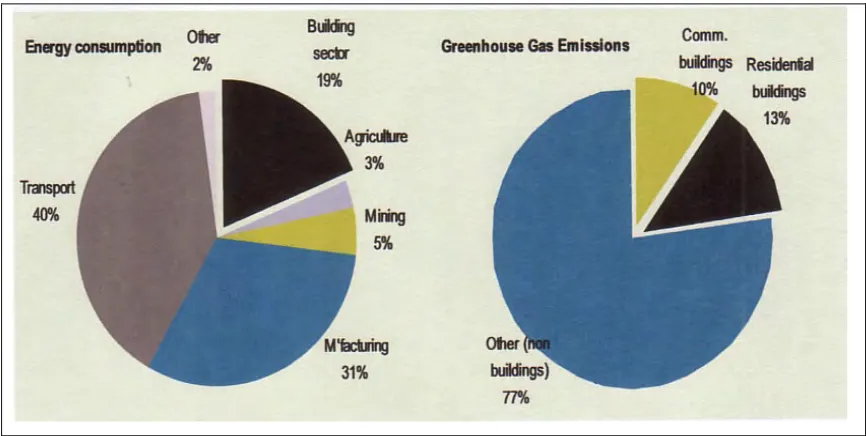
One of the international concerns was that buildings consume one third of the world’s resources (Atkinson 2006). In 2008, the Australian Sustainable Built Environment Council (ASBEC) reported that the building sector in Australia consumed about 19% of total energy, contributing a greenhouse gas emission of 23% of Australia’s total. Residential buildings were found to be responsible for emitting about 13% of greenhouse gas emission (Australian Sustainable Built Environment Council 2008).
The Australian government examined the building sector’s greenhouse gas emissions. They are detailed in the National Greenhouse Strategy document (Australian Greenhouse Office 1998a), which recommended that all commercial and residential buildings should adhere to energy efficiency standards based on thermal performance ratings. In 2003 the Building Code of Australia (BCA) introduced the first thermal performance requirements for residential buildings and mandated a minimum 4-star performance rating. This was increased to 5-stars in 2006 and 6-stars in 2010.
The introduction of the 4-star rating had a minimal impact on construction requirements. However, the move from 4 to 5 and 6-star conditions had considerable impact, especially on residential buildings using a timber platform floor construction. Various industry groups raised serious concerns about the new energy efficiency requirements, especially the construction cost implications and the accuracy of the simulation program used to assign star ratings. (Forest & Wood Products of Australia 2008; National Association of Forest Industries 2006).
The framework for several thermal modelling programs was established by the National House Energy Rating Scheme (NatHERS). Three software programs were endorsed, namely:
FirstRate;
BERS.
Each one of these programs can be used to demonstrate building energy efficiency compliance with the BCA. The AccuRate thermal simulation software, which was developed by the CSIRO, is used as the benchmark for accrediting other House Energy Rating Software (HERS). One of the major concerns raised by the industry was the accuracy of the star-rating program. The Housing Industry Association reported that builders regard the star-rating software as costly,’ green blinding’ and inherently unreliable (Hedley 2010). It also suggested that energy efficiency requirements created a multi-billion dollar component of the building and construction industry and those inaccurate star-rating assessments might result in a considerable financial burden to Australian home owners.
Williamson et al. (2001) reported that during the NatHERS development, no testing of the scheme against reality was conducted, and further stated that the star-rating is meaningless, as there is no correlation between star-ratings and household energy consumption and greenhouse gas emissions.
Further criticism of the AccuRate software model was expressed by the National Association of Forest Industries (NAFI) in March 2006, which noted that AccuRate’s simulation of energy loads might be flawed. NAFI further stated, ‘Clearly the lack of validation of the computer modelling against the actual performance of current building materials and practices is of critical concern to the timber industries’ (National Association of Forest Industries 2006).
As a result of the concerns regarding the accuracy of the AccuRate software, the CSIRO, together with industry representatives and federal government agencies, agreed that the House Energy Rating Scheme (HERS) AccuRate should be validated empirically, comparing simulated values with measured values in a test building. The validation would then inform industry and government of the capability of AccuRate to predict room temperature, star-ratings and energy loads in buildings. An acceptable correspondence between simulated and measured values would provide industries with confidence in the program, while large variations between simulated and measured values would direct software developers to areas of the software requiring further improvements.
Consequently, the Five Star Thermal Performance project was initiated in 2005 by the Centre for Sustainable Architecture with Wood (CSAW) within the University of Tasmania’s School of Architecture & Design, with funding from the Forest & Wood Products Research & Development Corporation (FWPRDC) and the Australian Greenhouse Office (AGO).
This research project aimed to validate empirically the performance of the House Energy Rating Software AccuRate, using industry-standard types of building construction. Initially, this project was known as the No Bills and Five Star House project; it involved the construction and monitoring of three test houses at Mornington, Hobart, Tasmania. The houses were designed by the Launceston home developer CG&M Design Pty.Ltd. and were to be:
The No Bills House, with an 8.5-star rating, having no external service requirements;
The Best Five Star Timber Floor House with an enclosed subfloor; and
The Best Five Star Concrete Floor House with a concrete slab-on-ground floor construction.
For financial reasons the original concept did not proceed. However, the proposal was reformulated into the Five Star Thermal Performance project. In this new proposal, two sets of test buildings were designed and constructed: three light-weight timber-framed test cells in Launceston and three 2-bedroom light-weight timber framed houses in Hobart, Tasmania.
The aim of this research project is to validate empirically the AccuRate software by monitoring the thermal performance of three test houses in a cool temperate climate area of Australia.
While a similar project validated AccuRate empirically, using three light-weight timber framed test cells, this is the first empirical zone temperature validation of AccuRate using purpose-built light-weight timber framed houses.
Arising from the aim of the research project, the research question is: How well does the AccuRate software predict indoor room temperatures in houses located in the cool temperature climate zones of Australia?
The research project’s hypothesis is: AccuRate’s simulated temperatures will be similar to measured temperatures in the three test houses.
Specifically, the objective of this research project is to compare AccuRate’s simulated hourly indoor temperatures with measured internal hourly temperatures for the three purposes-built houses in Kingston, Tasmania.
The key components of this research are presented as follows:
Chapter 2 discusses the history of climate change issues, Australia’s greenhouse gas emissions and Australian’s response to climate change. This chapter also focuses on the strategies for Australia’s building industries to reduce their greenhouse gas emissions. Finally, this chapter summarises house energy rating schemes in developed countries and concludes with a detailed description of Australia’s house energy rating schemes, in particularly the House Energy Rating Software, AccuRate.
Chapter 3 describes the methods used to validate simulation programs. This chapter examines empirical validation methods and establishes the important factors constituting a successful empirical validation project. A number of validation case studies of previously completed projects overseas and in Australia are briefly described.
Chapter 5 illustrates the design and construction of the three test houses in Kingston, Tasmania. The first part explains the star-rating process for each house while the second part provides a detailed presentation of the construction details of the houses.
Chapter 6 is presented in three parts:
Part 1 focuses on the description of the thermal monitoring equipment and the positioning of the sensors within the houses.
Part 2 provides a detailed illustration of the installation of sensors and cables inside the houses.
Part 3 addresses the data management, including their storage, cleaning and checking.
Chapter 7 explains AccuRate’s thermal performance simulation of the test houses. It covers the changes made to AccuRate’s input data that were necessary to provide a more realistic representation of the construction details and actual on-site weather conditions. In addition, this chapter describes the changes made to input files to simulate the free-running operation that is, (no heating and/or cooling) of the houses, when the houses were not occupied. Finally, the chapter concludes with a detailed description of the preparation of site climate data for AccuRate simulation.
Chapter 8 is presented in three parts:
Part 1 examines whether air or globe temperatures should be used for the validation of AccuRate.
Part 2 presents the graphical comparison of simulated and measured temperatures. Measured and simulated temperature profiles and daily maximum and minimum temperatures are shown graphically for selected zones of the houses. Finally, temperature ranges and differences between simulated measured values are compared between the houses, as a means of examining temperature trends.
Part 3 focuses on a more in-depth statistical analysis of the empirical validation data, and the differences between simulated and measured temperatures, particularly examining the residual values (the difference between measured and simulated temperatures) for each zone of the houses.
The conclusion and areas recommended for further research are discussed in Chapter 9.
Chapter 2: Climate Change and the Construction Sector
This chapter presents an overview of the global problem of increased greenhouse gas emissions, anticipated climate changes and the global action to reduce greenhouse gas emissions. It focuses on Australia’s response to greenhouse gas emission abatement strategies, particularly in the context of the building industry. In addition, this chapter reviews some of the House Energy Rating tools available and finally, provides a brief overview of the Australian House Energy Rating Tool “AccuRate”.
2.1. History of the Climate Change Issue
In 1950, scientist Roger Revelle formed a hypothesis that World War II, economic expansion, explosive population growth and fast growing energy consumption were likely to produce a dangerous increase in the amount of carbon dioxide (CO2) in the earth’s atmosphere (Gore 2006). Revelle proposed and designed a scientific experiment to collect samples of CO2 high in the Earth’s atmosphere at numerous locations. In 1957, together with Charles Keeling, Revelle established the first research station at the top of Mauna Loa, a volcanic mountain at Hawaii, USA. This location in the middle of the Pacific Ocean was chosen so that test air samples would not be contaminated by industrial emissions. In 1958 Revelle and Keeling began launching weather balloons and analyzing the amount of CO2 in the air samples they collected every day. After the first few years of taking air samples, the trend of rising CO2 levels in the atmosphere had already become clear (Gore 2006).
Figure 2.1 indicates rising CO2 concentration in the atmosphere (from 317ppm to 365ppm), measured at an altitude of about 4000 meters, on the top of Mauna Loa Mountain in Hawaii, from 1959 to 1998.
In 1987, the Brundtland Report, also known as ‘Our Common Future’, linked economic development and the need to sustain it without depleting natural resources or harming the environment. This report provided a key statement on sustainable development, defining it as: “Development that meets the need of the present without compromising the ability of future generation to meet their own needs” (Brundtland 1987, p. 43).
The Brundtland Report was concerned with securing global equity and the redistribution of resources towards poorer nations, whilst encouraging economic growth. The report also suggested that equity, growth and environmental maintenance are possible and that each country is capable of achieving its full economic potential without diminishing its resources. This report also highlighted three fundamental components of sustainable development: environmental protection, economic growth and social equity. The environment should be conserved and our resources enhanced by progressively changing the traditions in which we develop and use technologies. Developing nations must be allowed to meet their basic needs of employment, food, energy, water and sanitation. If this is to be done in a sustainable manner, there is a specific need for a sustainable level of population. Economic growth should be encouraged and developing nations should have the same growth opportunities as developed nations.
In 1988, the World Meteorological Organization (WMO) and the United Nations Environmental Program (UNEP) established the Intergovernmental Panel on Climate Change (IPCC). The purpose of the IPCC was to evaluate the state of knowledge on various aspects of climate change, including the science, environmental and socio-economic impacts and response strategies. The IPCC is recognized as the most authoritative international source of scientific, technical and socio-economic advice on climate change issues. It completed the first Assessment Report in August 1990, which was used as the basis for negotiating the United Nations Framework Convention on Climate Change (UNFCCC). The UNFCCC organized the United Nations Conference on Environment and Development (UNCED), which took place in 1992 in Rio de Janeiro, Brazil. The main objective was to stabilize greenhouse gases in the atmosphere to a level that would prevent anthropogenic interference with the climate system. Representatives from developing nations emphasized the importance of their right to economic development and argued that industrialized nations have special responsibilities to stabilize greenhouse gas emissions.
emission to 1990 levels by the year 2000, and that all nations would undertake voluntary actions to measure, report and limit their greenhouse gas emissions.
In the second Assessment Report of the IPCC (1995) the summary stated:
Climate has changed over the past century;
The balance of evidence suggest a discernible human influence on global climate;
Climate is expected to continue to change in the future as the concentration of greenhouse gases in the atmosphere increases;
For many regions and systems, the effects of climate change are likely to be adverse;
There are still many uncertainties.
Scientific evidence points out that human activity is having an adverse impact on the global climate system, including contributing to global warming. It also became apparent that major nations would not meet the voluntary arranged targets by 2000. The parties to the treaty of the UNFCCC decided (in 1995), that it would be necessary to enter into a legally binding treaty rather than a voluntary agreement to reduce greenhouse gas emissions.
The objective of the Kyoto Climate Change conference was to enter into a legally binding international agreement, where all participating nations are committed to reducing global warming and greenhouse gas emissions. The protocol was initially adopted at the Kyoto Climate Change Conference on December 11, 1997 and took force on February 2005. The five principal concepts of the Kyoto Protocol (Fletcher 2004) were:
Commitments to reduce greenhouse gases that are legally binding for Annex 1 countries (38 developed nations), as well as general commitments for all member countries;
Implementation to meet the Protocol’s objectives, to prepare policies and measures that reduce greenhouse gases, increase absorption of these gases and use all mechanisms available, such as: joint implementation, clean development mechanism and emissions’ trading; being rewarded with credits, which allows more greenhouse gas emission at home;
Minimize impacts on developing countries by establishing an adaptation fund for climate change;
Accounting, reporting and review to ensure the integrity of the protocol;
As from February 2009, 183 states have signed and ratified the Protocol (United Nations Framework Convention on Climate Change 2009). Under the Protocol, industrialized countries agreed to reduce their collective greenhouse gas emission by 5.2% from the 1990 level. National limitations range from: the reduction of 8% for the European Union and others, to 7% for the United States, 6% for Japan and 0% for Russia. The Kyoto Protocol permitted an emissions increase of 8% for Australia and 10% for Iceland. The United States, although a signatory to the Kyoto Protocol, has neither ratified nor withdrawn from the protocol. Australia signed the ratification on December 3, 2007 and it took effect on March 11, 2008.
The Copenhagen Climate Change conference, known as the Copenhagen Summit, was held in Copenhagen, Denmark, on December 7, 2009. The initial major goals of this conference included: greenhouse gas reduction by developed countries, agreements on how to monitor reduction commitments, and how to fund reduction of greenhouse gas emissions for developing countries.
The Copenhagen Agreement was drafted by the US, China, India, Brazil and South Africa on December 18, 2009 and was recognized, but not agreed upon, by all participating countries. The Agreement recognized that climate change is one of the greatest challenges of the present: therefore, action should be taken to keep the global temperature increase to 2ºC, to prevent the worst effects of climate change. However, this agreement does not contain any legally binding commitments that will result in reductions in CO2 emissions (BBC News 2009).
2.2. Australia’s Greenhouse Gas Emission and Response to the
Climate Change Issue
It can be seen in Figure 2.2 that Australia’s greenhouse gas emissions have grown from 480 million CO2-e in 1999, to 552 million CO2-e in 2009, an increase of 13.1% (Australian Government Department of Climate Change 2009).
Australia’s contribution to global greenhouse gas emissions is very small, at approximately 1.4% (Young 2007). However, on a per capita basis, with only 0.32% of the global population, Australia emits 1.43% of the world’s CO2 emission and is one of the highest emitters per capita in the world (Holper & Torok 2008). Table 2.1 represents a comparison of Australia’s annual emission between March 2008 and March 2009 and provides a breakdown of the individual sources of greenhouse gas emissions.
Table 2.1: Australia’s annual greenhouse gas emission between March 2008 and March 2009 (Source: Department of Climate Change 2009)
In 1992, Australia developed the first National Greenhouse Response Strategy, involving voluntary cooperation and participation by different levels of government, industry and the community, with the aim of reducing greenhouse gas emissions (Greenhouse Challenge Agreement). Also in December 1992, Australia ratified the UNFCCC agreement. In 1995, Australia accepted and endorsed the second assessment report of the IPCC. Before the Kyoto meeting, the Australian government moved from a voluntary approach to a more proactive strategy to address the rising greenhouse gas emissions. In November 1997, the then Prime Minister of Australia John Howard announced a major statement entitled “Safeguarding the Future, Australia’s Response to Climate Change”. This included an $180 million package of greenhouse gas reduction initiatives and measures addressing climate change and greenhouse gas emission issues. The Australian Greenhouse Office (AGO) was established in 1998 with the role of reducing greenhouse gas emissions. In the same year the AGO published the National Greenhouse Strategy Report (Australian Greenhouse Office 1998). This report focused on three major areas:
Implementing the awareness and understanding of greenhouse issues;