Distributed Fair Allocation of Indivisible Goods
IYann Chevaleyrea, Ulle Endrissb, Nicolas Maudetc
aLIPN, Universit´e Paris-Nord, France bILLC, University of Amsterdam, The Netherlands
cLIP6, Universit´e Pierre et Marie Curie, France
Abstract
Distributed mechanisms for allocating indivisible goods are mechanisms lacking central control, in which agents can locally agree on deals to exchange some of the goods in their possession. We study convergence properties for such distributed mechanisms when used as fair division procedures. Specifically, we identify sets of assumptions under which any sequence of deals meeting certain conditions will converge to a propor-tionally fair allocation and to an envy-free allocation, respectively. We also introduce an extension of the basic framework where agents are vertices of a graph representing a social network that constrains which agents can interact with which other agents, and we prove a similar convergence result for envy-freeness in this context. Finally, when not all assumptions guaranteeing envy-freeness are satisfied, we may want to minimise the degree of envy exhibited by an outcome. To this end, we introduce a generic framework for measuring the degree of envy in a society and establish the computational complexity of checking whether a given scenario allows for a deal that is beneficial to every agent involved and that will reduce overall envy.
Keywords: multiagent systems, multiagent resource allocation, fair division, negotiation, social networks
1. Introduction
The problem of fairly dividing a number of goods between several agents has been studied in a variety of settings. First, we may distinguish allocation problems fordivisible and forindivisible goods. The literature on cake cutting, for instance, is concerned with divisible goods [3, 4, 5]. As for indivisible goods, we can distinguishassignment problems [6], where each agent can consume at most a single good, from more general settings where each agent may receive a set (or bundle) of goods [7, 8, 9]. If agents can receive sets of goods, and if their preferences over the goods are not additively separable, then fair division becomes a combinatorial optimisation problem. We may also distinguish whether or not to allow for monetary side payments to be added to the bundles allocated to the agents, and if so we have to decide what assumptions to make regarding the agents’ appreciation of money (such asquasi-linearity, for instance). Finally, there are many different ways in which to interpret the termfairness itself [10]. For instance, we may be interested in equitable allocations, in proportional allocations, or in allocations where agents do not envy each other. In this paper, we adopt a model where sets of indivisible goods need to be allocated to a number of agents; agents express their preferences in terms of valuation functions over sets of goods; and side payments are possible and agents have quasi-linear preferences regarding money. We focus on two fairness criteria: first, we look for solutions that areproportionally fair (i.e., where the utility of each of then agents is at least 1/nth of the value she ascribes to the full set of goods) and, second, we look forenvy-free solutions (where no agent envies any of the other agents). (These criteria will get formally defined in Sections 3 and 4.)
While fair division is a problem originating in Economics and Political Science, with a number of impor-tant contributions by mathematicians, it eventually also started to attract the attention of researchers in Artificial Intelligence, Multiagent Systems, and Theoretical Computer Science [11, 12, 13, 14, 15, 16, 9, 5]. The reason for this trend is twofold: first, concepts from fair division are immediately relevant to these dis-ciplines (e.g., finding acceptable agreements in a multiagent system) and, second, the tools and techniques of these disciplines can shed new light on previously unexplored aspects of fair division (e.g., by applying ideas from complexity theory).
There is large variety concerning theproceduresthat have been proposed to address fair division problems. Some work emphasises that such procedures should be simple enough to be executable by humans. Others have concentrated on devising computationally efficient algorithms. Our own approach is to use adistributed mechanism in which agents can locally agree on deals to exchange some of the goods in their possession. In this approach, we initially choose a random allocation of goods to agents and then let the agents negotiate freely to, hopefully, find a superior allocation. Each agent’s preferences are defined using a (not necessarily additive) valuation function. Agents agree on a sequence of deals to exchange goods, which may be combined with monetary side payments. Once negotiation is underway, there is no central control regulating the process and agents are assumed to make deals according to their own preferences. Standard cake-cutting procedures that have been proposed for the fair partitioning of a single divisible good [3], for instance, are not distributed in this sense. While some of them, like, e.g., the well-known Banach-Knaster “last diminisher procedure”, do not require a referee to execute the procedure, they nevertheless proceed according to a fixed (global) protocol specifying which agent has to perform which type of action at any given time. The same is true for the “descending demand procedure” of Herreiner and Puppe [17], a procedure for finding equitable allocations of indivisible goods.
The kind of distributed approach followed here has been studied by several authors [18, 13, 19, 20, 21]. It is particularly attractive for large systems of autonomous software agents that need to negotiate an allocation of resources or agree on a distribution of tasks amongst themselves. Being able to distribute the computation of an optimal allocation of goods over the agents is useful in many applications where no central authority can be relied upon to eventually decide on the allocation. This may, for instance, be the case in view of computational limitations of a potential centre, or in view of its trustworthiness. In such a context the use of combinatorial auctions or similar mechanisms [22], which in principle could be employed to find an optimal allocation of indivisible goods, may be considered problematic. The same argument has also been made by Netzer et al. [23], who proposed a framework for finding fair allocations of goods based on distributed constraint optimisation. But even when we give up central control of the optimisation algorithm, as system designers, we still would want to try to set up the system in such way that it guarantees certain desirable properties, although now without directly interfering into the process of negotiation.
In this paper we study convergence properties for distributed allocation mechanisms when used as fair division procedures. Specifically, we identify sets of assumptions under which any sequence of deals meeting certain conditions can be shown to converge to a proportionally fair allocation and to an envy-free allocation, respectively. We also introduce an extension of the basic framework where agents are vertices of a graph (which we might think of as representing a social network) limiting which agents can interact with each other. The concept of envy-freeness is very naturally extended to such a setting: an agent will not envy another agent if they either believe that their own bundle is more valuable or if they cannot see that other agent, because there is no edge between them in the network. This allows us to prove a similar convergence result for envy-freeness in the context offair division on a graph. Finally, when not all assumptions guaranteeing envy-freeness are satisfied, it is interesting to study the degree of envy exhibited by an outcome. To this end, we introduce a generic framework for defining measures for assessing the degree of envy in a society and establish the computational complexity of checking whether a given scenario allows for a deal that is beneficial to every agent involved and that will reduce envy.
our setting and obtain a distributed procedure that guarantees convergence to a proportionally fair outcome. In Section 4 we carry out a similar programme, this time choosing envy-freeness as our goal. Envy-freeness is considerably more demanding a criterion than proportionality, so the convergence results that we obtain rely on somewhat stricter assumptions. The framework is extended to fair division on graphs in Section 5. We discuss possible extensions of the notions of efficiency, proportionality, and envy-freeness to this richer setting, and in the case of envy-freeness arrive at a particularly satisfying definition as well as an attractive convergence result. We also argue that proportionality and efficiency are not naturally generalised to this setting. Section 6 proposes a framework for assessing the degree of envy in a society. It also establishes a computational complexity result that shows that identifying a deal that is acceptable to each agent involved and that reduces envy is NP-complete (but not harder than finding a deal that is simply acceptable to the agents involved). This holds for all the concrete measures of envy we define, and indeed for a much larger class of such measures, defined by a simple axiom. Section 7 concludes.
2. Distributed mechanisms for allocating indivisible goods
In this section we define the class of distributed mechanisms that we want to employ to negotiate fair allocations of goods and briefly recall a number of known results [13, 18].
2.1. Agents, goods, allocations, valuations
Let N ={1, . . . , n} be a finite set of agents and let G, with m =|G|, be a finite set of indivisible goods. Anallocation A :N →2G is a partitioning of the items in G amongst the agents in N, i.e., each good is owned by exactly one agent (here 2G denotes the powerset of G). As an example, allocationA, defined via A(i) ={g1} andA(j) ={g2, g3}, would allocateg1 to agenti, andg2 andg3 to agentj. We assume that
the initial allocation, denoted byA0, has been chosen at random, so agents cannot derive any rights from
this allocation (as far as the definition of fairness is concerned).
The interests of individual agentsi ∈ N are modelled usingvaluation functions vi : 2G →R, mapping
bundles of goods to the reals. Valuation functions are private information. However, we assume that when asked for the valuation of a given bundle of goods S, any agent i will truthfully reveal the value vi(S)
she assigns to S. To simplify presentation, throughout this paper, we will make the assumption that all valuationsvi arenormalised, in the sense that vi(∅) = 0, andnon-negative, meaning thatvi(S)>0 for all
S⊆ G. We sometimes usevi(A) as a shorthand forvi(A(i)), the value agentiassigns to the bundle received
in allocationA.
Some of our results only apply to scenarios where all valuation functions meet additional properties. A valuation function is calledmodular (oradditive) if v(S1∪S2) =v(S1) +v(S2)−v(S1∩S2) for all bundles
S1, S2⊆ G. Similarly,vis calledsupermodular ifv(S1∪S2)>v(S1) +v(S2)−v(S1∩S2). Finally, a valuation
function is calledsingle-minded if there exist a bundle S∗⊆ G and a positive numbercsuch that v(S) =c in caseS∗⊆S andv(S) = 0 otherwise. Thus, in a single-minded agent is only interested in a single bundle of goods and assigns a fixed value to that bundle (and to all larger bundles including that specific bundle as a subset).
2.2. Deals, payments, utility
Agents negotiate sequences of deals to improve their own welfare. Adeal δ= (A, A0) is a pair of allocations (withA 6=A0), specifying the situation before and after the deal. Observe that a single deal may involve the reassignment of any number of goods amongst any number of agents. A1-deal is a deal involving only a single good (and hence only two agents). The set of agents involved in the dealδ= (A, A0) is denoted as Nδ ={i∈ N |A(i)6=A0(i)}. (In Section 5 we will introduce a refinement of the basic model, where agents
can only make deals with agents to which they are connected in an underlying negotiation topology.) Deals may be accompanied by monetary side payments to allow agents to compensate others for otherwise disadvantageous deals. This is modelled using so-calledpayment functions: p:N →R, which are required
to satisfy P
ip(i) = 0. A positive value p(i) indicates that agent i pays money, while a negative value
{g1} {g2} {g3} {g4} {g1, g2, g3, g4}
Agent 1 5 5 0 0 10
Agent 2 4 4 4 4 18
Agent 3 0 0 5 5 10
Table 1: Valuation functions for an “almost modular” 3-agent/4-good allocation problem
a function π: N → R mapping agents to the sum of payments they have made so far, i.e., we also have
P
iπ(i) = 0. Astateof the system is a pair (A, π) of an allocationAand apayment balanceπ. It is possible
to impose aninitial payment on each agent, at the time of awarding them the bundle they receive in the initial allocation. Payment function and initial payments together are referred to as thepayment scheme.
Each agenti∈ N is also equipped with autility function ui : 2G×R→Rmapping pairs of bundles and
previous payments to the reals. These are fully determined by the valuation functions: ui(S, x) =vi(S)−x.
That is, utilities arequasi-linear: they are linear in the monetary component, but the valuation over bundles of goods may be any set function. For example,ui(A(i), π(i)) is the utility of agentiin state (A, π), while
ui(A(j), π(j)) is the utility that iwould experience if she were to swap places withj (in terms of both the
bundle owned, and the sum of payments made so far).
2.3. Individual rationality and efficiency
Agents are assumed to only negotiate individually rational (IR) deals, i.e., deals that benefit everyone involved:
Definition 1 (IR deals). A deal δ= (A, A0) is called individually rational (IR) if there exists a payment function p such that vi(A0)−vi(A)> p(i) for all agents i∈ N, except possibly p(i) = 0 for agents i with
A(i) =A0(i).
While negotiation is driven by the individual preferences of agents, we are interested in reaching states that are attractive from a “social” point of view. A common measure for efficiency is (utilitarian) social welfare [24]:
Definition 2(Social welfare). The social welfare of an allocationA is defined as sw(A) =P
i∈Nvi(A(i)).
We also speak of the social welfare of astate (A, π). As the sum of allπ(i) is always 0, the two notions coincide, i.e., it does not matter whether we define social welfare in terms of valuations or in terms of utilities. A state/allocation with maximal social welfare is calledefficient.
Example 1. Let us consider an allocation problem with three agents, N ={1,2,3}, and four goods,G = {g1, g2, g3, g4}. Table 1 defines the valuation functionsvi by indicating for each agent how much she values
the four individual goods and how much she values the full bundle. The values of bundles not shown are assumed to always be equal to the sum of the values of the items in them. Thus,v1 andv3are modular, and
all three valuation functions are supermodular.
Maximal social welfare for this allocation problem is20, namely when agent 1 holds the bundle{g1, g2},
agent 2 gets nothing, and agent 3 holds {g3, g4}. Let us denote this optimal allocation by A∗. Suppose
now we are in allocationA, in which all four items are held by agent 2. Social welfare forA is 18. If our agents are only willing to negotiate 1-deals, then we will remain stuck in this suboptimal allocation and never reachA∗. To see this, check that agent 2 giving any single item to one of the other two agents would result in a drop of her utility from18to12, thus requiring a price strictly above6, which neither one of the other two agents would be willing to pay. We will return to this example throughout this paper.
A central result in distributed negotiation, due to Sandholm [18], shows that the problem we observed in Example 1 does not persist if we do not impose any structural constraints on deals:
That is, if agents continue to agree on IR deals, they will eventually reach a state from which no further IR deal is possible, and that state will be efficient. This result guarantees that agents can agree on any sequence of deals meeting the IR condition without getting stuck in a local optimum; and there can be no infinite sequence of IR deals. On the downside, this result presupposes that agents are able to negotiate complex multilateral deals between any number of agents and involving any number of goods. In modular domains, we can get a much stronger convergence result [13]:
Theorem 2 (Efficient outcomes by 1-deals). If all valuation functions are modular, then any sequence of IR 1-deals will eventually result in an efficient allocation.
Theorems 1 and 2 are easy consequences of the fact that a move from one allocation to another is an IR deal if and only if that move increases social welfare (see Endriss et al. [13] for a proof):
Lemma 3(IR deals and social welfare). A dealδ= (A, A0)is IR if and only if sw(A)< sw(A0).
We will frequently rely on this fact in the sequel, mostly without explicit reference to Lemma 3. Note that Lemma 3 also entails that we can always reach an efficient allocation by means of just a single IR deal. Importantly, this does not diminish the importance of Theorem 1. Finding that particular IR deal to reach the optimum in a single step requires full coordination between all agents, while Theorem 1 guarantees convergence also in the absence of such global coordination and only requires agents to make deals locally that benefit themselves then and there.
2.4. Specific payment functions
Requiring deals to be IR puts restrictions on what deals are possible at all and it limits the range of possible payments, but it does not determine the precise side payments to be made. This is a matter to be negotiated by the participating agents. Estivie et al. [25] introduce several concrete payment functions that agents may choose to adopt. The two simplest ones are thelocally uniform payment function (LUPF) and theglobally uniform payment function (GUPF).
Choosing a payment function amounts to choosing how to distribute the social surplus sw(A0)−sw(A) generated by a dealδ= (A, A0). By Lemma 3, the social surplus is positive if and only ifδis IR. The LUPF divides this amount equally amongst theparticipating agentsNδ; the GUPF divides it equally amongstall
agentsN:
LUPF: p(i) = [vi(A0)−vi(A)]−[sw(A0)−sw(A)]/|Nδ|
ifi∈ Nδ and 0 otherwise
GUPF: p(i) = [vi(A0)−vi(A)]−[sw(A0)−sw(A)]/n
Importantly, note that the social surplus sw(A0)−sw(A) can always be computed from the valuation functions of the participating agents alone:
sw(A0)−sw(A) = X
i∈Nδ
[vi(A0)−vi(A)]
Thus, the LUPF is a fully local payment function: it only requires us to consider input from the participating agents and only the payment balances of these agents will be affected. The GUPF is also local as far as the information required is concerned, except that we need to know the quantitynbefore we can compute it. On the other hand, the GUPF is global in the sense that payment balances of all agents are affected. Having said this, agents not participating in the deal can only ever receive money, but never have to make a payment themselves.
3. Proportional fairness and Knaster payments
Definition 3 (Proportionality). A negotiation state(A, π)is called proportional if ui(A, π)>vi(G)/n for
all agentsi∈ N.
Proportionality is the central fairness criterion applied in the cake-cutting literature, which addresses the problem of fairly dividing a single divisible good [3, 4, 5]. Before we proceed, let us briefly pause and consider under what circumstances proportionality is a reasonable fairness concept also in our context. Importantly, in almost all of the cake-cutting literature, agents are assumed to haveadditive preferences, which is an assumption we do not always want to make. As a minimum requirement for Definition 3 to be meaningful, we need to make the assumption that valuation functions aremonotonic: S1⊆S2 implies
vi(S1) 6 vi(S2). When agent valuations are supermodular, then it will often be impossible to obtain a
proportional solution without using money (both for divisible and indivisible goods), because 1/nth of the value of the full set of goods would often be considered more than the value of 1/nth of the goods. For submodular valuations, on the other hand, proportionality would be a very undemanding fairness criterion, as it would often be easy to give an agent 1/nth of the value they ascribe to the full set by handing them a very small bundle. It is therefore questionable whether proportionality should be considered a relevant fairness criterion in case valuations may be submodular. This caution not withstanding, due to the central importance of proportionality in the classical literature, we nevertheless choose to demonstrate here how to apply our methodology to this concept. We will be able to obtain a positive result for arbitrary domains, but the reader should keep in mind that this result is at its most attractive when applied to supermodular rather than to submodular domains.
To define a distributed procedure that can guarantee proportional outcomes we will take inspiration from the classical fair division procedure proposed by Bronis law Knaster in the 1940s [26, 3, 27].1 In this section,
we recall the classical Knaster procedure, show how to adapt it to define a payment scheme, and prove a convergence theorem showing that this scheme guarantees outcomes that are both efficient and proportional.
3.1. The Knaster procedure
Our exposition of the Knaster procedure follows Raith [27]. An important difference between the classical and our (more general) setting is that in the classical setting valuation functions are assumed to be modular (additive). This difference affects the first step of the procedure.
(1) Compute an allocationA∗ that maximises social welfare. (In the classical setting this step simplifies to assigning each good to the agent who values it the most.)
(2) For each agenti, compute herexcess exi(A∗) =vi(A∗)−vi(G)/nover her fair share. Thetotal excess
is defined asEx(A∗) =P
iexi(A∗).
(3) Split the total excess evenly amongst all the agents; that is, require a payment ofexi(A∗)−Ex(A∗)/n
from each agenti.
Note that the individual excess of an agent could be a negative number, as could be the payment she has to make (in which case she would receive money). Clearly, the payments of all agents sum up to zero, so are feasible. While an agent’s individual excess exi could be negative, the total excessEx(A∗) will always be
positive (or zero). This follows from the fact thatEx(A∗) =sw(A∗)−1 n·
P
ivi(G) and that we must have
sw(A∗)>vi(G) for anyi(becauseA∗ is efficient by definition and hence at least as good as giving all goods
to i). After the procedure has been executed, agent i will enjoy utility vi(A∗)−[exi(A∗)−Ex(A∗)/n] =
vi(G)/n+Ex(A∗)/n. Hence, the Knaster procedure does indeed produce a proportional outcome.
3.2. Definition of a payment scheme
As demonstrated by Theorem 1, our distributed negotiation procedure is capable of selecting an allocation A∗ with maximal social welfare. We now want to devise a payment scheme that guarantees proportionality on top of efficiency. At the point of convergence we would like to obtain an outcome that is equivalent to the outcome we would have gotten by using the Knaster procedure.
Recall that defining a payment scheme involves fixing an initial paymentπ0(i) for each agent and choosing
a payment function p. Our approach is simply to choose π0 and psuch that at each stage (A, π) of the
negotiation we will have π(i) = exi(A)−Ex(A)/n, thereby emulating the payments prescribed by the
Knaster procedure (with the crucial difference that in the Knaster procedure payments are only required once, at the very end). LetA0be the initial (randomly chosen) allocation. We must fixπ0as follows:
π0(i) = exi(A0)−Ex(A0)/n (1)
Hereexi andEx are defined as in Section 3.1. Of course, ifA0 is sufficiently close to an efficient allocation,
then these payments will already result in a proportional outcome. On the other hand, for a sufficiently inefficientA0neither these nor any other payments could possibly ensure proportionality.
Next we choose a payment function p. We want to maintainπ(i) =exi(A)−Ex(A)/n as an invariant
for all negotiation states (A, π). This forces the following payments for a dealδ= (A, A0), withπbeing the payment balance for allocationAandπ0 being the payment balance forA0:
p(i) = π0(i)−π(i)
= [exi(A0)−Ex(A0)/n]−[exi(A)−Ex(A)/n]
= [vi(A0)−vi(A)]−[sw(A0)−sw(A)]/n
But this is exactly the GUPF, defined in Section 2.4. In particular, the payments prescribed by this choice of pare IR. In summary, theKnaster payment scheme is given by the GUPF together with the initial payments defined in Equation (1).
3.3. Convergence
We are now going to show that, indeed, negotiation using the Knaster payment scheme will always converge to a proportional outcome.
Theorem 4 (Proportional outcomes). Under the Knaster payment scheme, any sequence of IR deals will eventually result in a state that is efficient and proportional.
Proof. By Theorem 1, any sequence of IR deals must converge to an efficient state, independently from the specific payment scheme in use. As we are using the Knaster payment scheme, any state (A, π) reached during negotiation will satisfyπ(i) =exi(A)−Ex(A)/n for each agenti. Hence, we are bound to converge
to a state (A∗, π∗) with an efficient allocationA∗ where π∗(i) =exi(A∗)−Ex(A∗)/n. This is exactly the
kind of outcome we would have obtained had we used the Knaster procedure, which we have seen to always be proportional (see Section 3.1).
Thus, convergence to a proportional outcome is guaranteed. If all agents have modular valuation func-tions (as is the case for the classical setting of the Knaster procedure), then we can guarantee convergence to a proportional state using a simpler negotiation protocol.
Theorem 5 (Proportional outcomes by 1-deals). Under the Knaster payment scheme, if all valuation functions are modular, any sequence of IR 1-deals will eventually result in a state that is efficient and proportional.
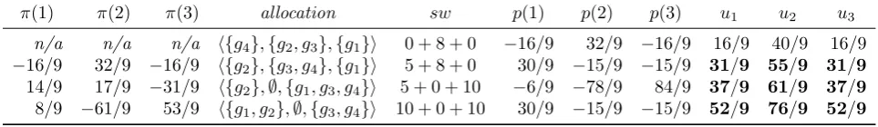
π(1) π(2) π(3) allocation sw p(1) p(2) p(3) u1 u2 u3
n/a n/a n/a h{g4},{g2, g3},{g1}i 0 + 8 + 0 −16/9 32/9 −16/9 16/9 40/9 16/9
−16/9 32/9 −16/9 h{g2},{g3, g4},{g1}i 5 + 8 + 0 30/9 −15/9 −15/9 31/9 55/9 31/9
14/9 17/9 −31/9 h{g2},∅,{g1, g3, g4}i 5 + 0 + 10 −6/9 −78/9 84/9 37/9 61/9 37/9
[image:8.595.63.545.113.183.2]8/9 −61/9 53/9 h{g1, g2},∅,{g3, g4}i 10 + 0 + 10 30/9 −15/9 −15/9 52/9 76/9 52/9
Table 2: Sequence of states using the Knaster payment scheme
Example 2. Recall Example 1, with three agents with valuation functions as specified in Table 1. The only efficient allocation here is A∗, which assigns {g
1, g2} to agent 1 and {g3, g4} to agent 3 and which has a
social welfare of 20. We may write this more compactly as A∗ =h{g1, g2},∅,{g3, g4}i. Suppose the initial
allocation isA0=h{g4},{g2, g3},{g1}i, giving utility0,8, and0 to agents 1, 2, and 3, respectively.
Let us illustrate convergence to a proportional allocation with Knaster payments. First, we compute the excess exi(A0) for each agenti:
• ex1(A0) = 0−10/3 =−10/3
• ex2(A0) = 8−18/3 = 6/3
• ex3(A0) = 0−10/3 =−10/3
The total excess Ex(A0)thus is6/3−10/3−10/3 =−14/3. The initial payments therefore must be:
• π0(1) =−10/3 + 14/9 =−16/9
• π0(2) = 6/3 + 14/9 = 32/9
• π0(3) =−10/3 + 14/9 =−16/9
It can readily be checked that, indeed, P
iπ0(i) = 0. At this stage, the state (A0, π0) is not proportional:
for instance, u1(A0(1), π0(1)) = 0 + 16/9 <10/3. Now suppose that, starting from this state, our agents
negotiate the sequence of states shown in Table 2. Each row corresponds to a state. The first three columns represent the payment balances before the state in question. Then the allocation and the social welfare are shown, followed by the new payments to be made in that state, in line with the Knaster payment scheme. Finally, the utility of each agent is shown. These utilities are indicated in boldface in case an agent has reached her “proportionality threshold” (which is 10/3 for agents 1 and 3, and 18/3 for agent 2). Observe that, for this example, all three agents surpass this threshold already after the second deal, i.e., efficiency is not always required to achieve proportionality.
We continue our treatment of proportionality by briefly discussing alternative payment schemes for guaranteeing proportional outcomes. As shown in Section 3.1, the Knaster procedure guarantees each agent ia marginal utility of Ex(A∗)/n above and beyond their fair share of v
i(G)/n. But any alternative
division of the total excess Ex(A∗) will also satisfy proportionality. The equal division chosen by Knaster
is a particularly natural choice, but it is not the only one. Raith [27], for instance, argues that a division of the total excess that is proportional to each individual’s valuation of the full set of goods may be more appropriate and proposes an adjustment of the Knaster procedure to achieve this.
Let (αi)i∈N with αi > 0 and Piαi = 1 be a vector specifying for each agent their entitlement to a
proportion of the total excess. By revisiting the proofs given above, it is not difficult to see that Theorems 4 and 5 will continue to hold if the Knaster payment scheme is replaced by any payment scheme of the following form:
π0(i) = exi(A0)−αi·Ex(A0)
p(i) = [vi(A0)−vi(A)]−αi·[sw(A0)−sw(A)]
For the Knaster payment scheme we have αi = 1n, while for the payment scheme corresponding to the
Raith-Knaster procedure [27] we have αi = Pvi(G)
3.4. Path length
In the previous section we have seen that convergence to an efficient and proportional state can always be guaranteed by our scheme. But how many deals do we require to reach a social optimum? First, observe that by Lemma 3, it is always possible to reach the optimum using (at most) one deal, i.e., 1 is a (tight) upper bound on the shortest path. Much more interesting in practice, however, is the longest path, i.e., the longest sequence of IR deals that agents may end up agreeing on before convergence. For convergence to an efficient allocation by means of IR deals,nm−1, withnbeing the number of agents andmbeing the number of goods, is known to be a (tight) upper bound on the longest path, i.e., there exist profiles of valuation functions and initial allocations such that it is possible to visit all allocations before convergence [29]. Inspection of the proof of that result shows that it does not depend on the payment scheme used. Hence,nm−1 is
also an upper bound on the number of deals for scenarios covered by Theorem 4—at least if we do not put restrictions on the nature of our agents’ valuation functions.
If we do require valuation functions to be normalised and monotonic (and possibly also supermodular, which we have argued to be reasonable in the context of studies of proportionality), then the construction used in previous work [29] does not apply any longer. We now want to show that the result itself nevertheless carries over.
Lemma 6 (Distinct welfare). We can find a valuation function for each agent that is normalised, non-negative, and modular such that any two allocations have distinct utilitarian social welfare.
Proof. We first define the valuation functionv1 of the first agent in a way that ensures that she assigns a
distinct value to every possible bundle. LetG={g1, . . . , gm}and define:
v1(S) =
X
g∈S
ν(g) withν(gk) = 2k−1
That is,v1maps bundles to the numbers from 0 to 2m−1 (the reader may find it helpful to think of bundles
as representing binary numbers with m digits). Note that v1 is normalised, non-negative, and modular.
Now define the valuation functions of the remaining agents as follows:
vi(S) = v1(S)·(2m)i−1
That is, each agent’s valuation function is operating “at its own scale”. Now, if we are given the utilitarian social welfare of an allocationAas a binary number, then we know that that number will have a 1 in position m·(i−1) +k(counting from the right) if and only if agentihas obtained goodgk underA. Hence, there is
a bijection between allocations and social welfare values, i.e., any two distinct allocations must have distinct social welfare, as claimed.
Observe that any valuation function that is normalised, non-negative, and modular is also monotonic and supermodular. Hence, there exist normalised, monotonic and supermodular valuation functions such that no two allocations have the same utilitarian social welfare. This means, that there exists a sequence of IR deals that visits allnm allocations (each of the m goods may be given to any of the nagents), and thusnm−1 is a tight upper bound on the length of the longest path for scenarios covered by Theorem 4, also when valuations are subject to the restrictions we have argued to be natural for studies of proportional fairness.
This bound applies in case we are interested in finding an allocation that is both proportional and efficient. Can we do better if we only require proportionality? This might seem a possibility, given the fact that, if agents negotiate IR deals using the Knaster payment scheme, then efficiency is only achieved at the very last deal, but proportionality will often get achieved already much earlier, namely as soon as the total excessEx(A) of the current allocationAis non-negative. Yet, the answer to our question is still negative:
Proof. Take a scenario where the agents have the valuation functions used in the proof of Lemma 6, except thatvn(G) is set to such a high value that the only way of achieving a proportional state is to give all goods
to agent n (because no payments the other agents would be prepared to make could be large enough to give utility vn(G)/n to agent n). Then all allocations have distinct social welfare, i.e., we can construct a
sequence of deals visiting all of them, and proportionality would only get achieved at the very end of the sequence.
Finally, given Lemma 6, known results for convergence by means of 1-deals in case all valuation func-tions are additive (i.e., the kind of scenario covered by Theorem 5) now also carry over immediately [29]. Concretely, this means thatm is a tight upper bound for the shortest path (as we need at most one deal per item if we only choose optimal deals) andm·(n−1) is a tight upper bound for the longest path (as each item may, in the worst case, pass through every single agent).
4. Envy-freeness and globally uniform payments
Besides proportionality, another important fairness criterion isenvy-freeness [30, 3, 11, 10]. An allocation of goods is envy-free if no agent would rather have the bundle held by one of the other agents. This is a more demanding requirement than proportionality. Indeed, if we require all goods to be allocated, then an envy-free allocation may not even exist at all, and the problem of checking whether or not an envy-envy-free allocation exists has been shown to be computationally intractable [14]. Fortunately, in the presence of money, when envy-freeness is defined in terms of both bundles of goods and payments received, the situation is more favourable and envy-free solutions do exist [7].
In this section we will identify conditions under which we can guarantee convergence to an envy-free outcome.
Definition 4(Envy-freeness). A negotiation state(A, π)is called envy-free ifui(A(i), π(i))>ui(A(j), π(j))
for all agentsi, j∈ N.
A state that is both efficient (in the sense of maximising social welfare) and envy-free will be referred to as anEEF state.
If all valuation functions are submodular (or modular), that is, when no agent ever likes the union of two disjoint bundles strictly more than the sum of the valuations of the two individual bundles, then any state that is envy-free is also proportional. The converse is not true: a proportional state is not necessarily envy-free. If valuation functions are supermodular, then envy-freeness does not guarantee proportionality, norvice versa.
4.1. Existence of envy-free states
In the presence of money, intuitively, chances for finding an envy-free solution are better than when there is no money. In particular, in the context of assignment problems, i.e., when each agent can only receive at most a single good, states that are both efficient and envy-free are known to always exist. This has been shown by Alkan et al. [6]. When agents can obtain (and express preferences over) bundles consisting of several goods, there is in general no such guarantee, i.e., as demonstrated by Tadenuma [8], for some allocation problems there simply exists no state that is both efficient and envy-free. However, the assumption of quasi-linearity of money is very important here: if we require quasi-linearity, as we do in this paper, then the existence of EEF states can be proven by an argument similar to the one used by Alkan et al. [6], appealing to the Duality Theorem [31], as demonstrated by Bevi´a [7]. When all valuation functions aresupermodular, we can give a much simpler argument for the existence of EEF states, which does not rely on the Duality Theorem. As we will see later on, this case is of special interest to us, which is why we present this argument here in some detail.
There clearly always exists an allocation that is efficient: some allocation must yield a maximal sum of individual valuations. LetA∗ be such an efficient allocation. We show that a payment balanceπ∗ can be arranged such that the state (A∗, π∗) is EEF. Defineπ∗(i) for each agenti:
First, note thatπ∗ is a valid payment balance: theπ∗(i) do indeed sum up to 0. Now let i, j ∈ N be any two agents in the system. We show thati doesnot envyj in state (A∗, π∗). AsA∗ is efficient, giving both A∗(i) andA∗(j) toiwill not increase social welfare any further:
vi(A∗(i)) +vj(A∗(j)) > vi(A∗(i)∪A∗(j))
Asvi is assumed to be supermodular (and normalised), this entails:
vi(A∗(i)) +vj(A∗(j)) > vi(A∗(i)) +vi(A∗(j))
Adding sw(A∗)/n to both sides of this inequality, together with some simple rearrangements, yields ui(A∗(i), π∗(i)) > ui(A∗(j), π∗(j)), i.e., agent i does indeed not envy agent j. Hence, (A∗, π∗) is not
only efficient, but also envy-free.
Of course, the mereexistenceof an EEF state alone is not sufficient in the context of negotiation amongst autonomous agents. Why should rational decision-makers accept the allocation and payments prescribed above? And even if they do, how can we compute them in practice? Just finding an efficient allocation is already known to be NP-hard [32]. Finally, as argued in the introduction, we are interested in adistributed procedure, where agents identify the optimal state in an interactive manner.
4.2. Convergence in supermodular domains
We are now going to prove a result on the reachability of EEF states by means of distributed negotiation. Our result applies to supermodular domains only. The payment scheme it employs consists of the GUPF in combination with the following initial payments:
π0(i) = vi(A0)−sw(A0)/n
That is, each agent has to first pay an amount equivalent to their valuation of the initial allocation A0,
and will then receive an equal share of the social welfare as a kick-back. We refer to this choice of initial payment as aninitial equitability payment. Note that this payment does not achieve envy-freeness (and it does not affect efficiency at all). In the special case where none of the agents has an interest in the goods they hold initially (vi(A0) = 0 for alli∈ N), the initial payments reduce to 0.
Theorem 8 (Envy-free outcomes). If all valuation functions are supermodular and if initial equitability payments have been made, then any sequence of IR deals using the GUPF will eventually result in an EEF state.
Proof. We first show that the following invariant will be true for every state (A, π) and every agent i, provided that agents only negotiate IR deals using the GUPF:
π(i) = vi(A)−sw(A)/n (2)
Our proof proceeds by induction over the number of deals negotiated. As we assume that initial equitability payments have been made, claim (2) will certainly be true for the initial state (A0, π0). Now letδ= (A, A0)
and assume (2) holds for A and the associated payment balance π. We obtain the payment balance π0
associated withA0 by adding the appropriate GUPF payments toπ:
π0(i) = π(i) + [vi(A0)−vi(A)]−[sw(A0)−sw(A)]/n
= vi(A0)−sw(A0)/n
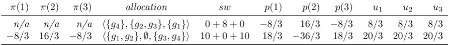
π(1) π(2) π(3) allocation sw p(1) p(2) p(3) u1 u2 u3
n/a n/a n/a h{g4},{g2, g3},{g1}i 0 + 8 + 0 −8/3 16/3 −8/3 8/3 8/3 8/3
[image:12.595.74.523.113.158.2]−8/3 16/3 −8/3 h{g1, g2},∅,{g3, g4}i 10 + 0 + 10 18/3 −36/3 18/3 20/3 20/3 20/3
Table 3: Convergence to an EEF state using equitability payments and the GUPF
Example 3. Observe that the final state attained in Example 2 is not envy-free. This is so, because, for instance,u1(A∗(1), πK(1)) = 52/9, whileu1(A∗(2), πK(2)) = 76/9: agent 1 envies agent 2, even though the
latter does not own any goods, because of the amount of money she receives through the Knaster payments (here,πK denotes the payment balances according to the Knaster scheme for the final state, corresponding to
the efficient allocationA∗=h{g1, g2},∅,{g3, g4}i). To illustrate the difference between the Knaster payment
scheme and the payment scheme of Theorem 8, let us consider the simple example shown in Table 3, involving the initial allocation A0 =h{g4},{g2, g3},{g1}i and a single IR deal leading to the efficient allocationA∗.
Note that the initial state is not envy-free, not even after the initial equitability payments, as for instance agent 2 envies agent 1, given thatu2(A0(1), π0(1)) = 4 + 8/3 = 20/3>8/3 = 8−16/3 =u2(A0(2), π0(2)).
As argued in Section 3.4, Lemma 6 shows that the bounds on the lengths of paths to convergence established in previous work on negotiating efficient allocation for arbitrary valuation functions [29] apply also to the types of scenarios covered by Theorem 8: 1 is a (tight) upper bound on the shortest path and nm−1 is a (tight) upper bound on the longest path.
Theorem 8 is a surprising result. As pointed out elsewhere [13], it is not possible to define a “local” criterion for the acceptability of deals (which can be checked taking only the valuation functions of the agents involved into account) that would guarantee that a sequence of such deals always converges to an envy-free state. We circumvent this problem here by using the GUPF, which adds a (very limited) non-local element. It is limited, because only the agents involved in a deal can ever be asked to give away money, and all payments can be computed taking only the valuations of those involved into account.
A natural question that follows is whether Theorem 8 could be generalised, namely whether a more general class of valuations would still allow us to guarantee convergence to an envy-free state. The following result shows that this is not the case, at least not if we keep the payment scheme of Theorem 8 in place.
Theorem 9(Maximality of supermodularity). No class F of valuation functions that strictly includes the class of supermodular functions can guarantee the following property: if all valuation functions are drawn from F and initial equitability payments have been made, then any sequence of IR deals using the GUPF will eventually result in an EEF state.
Proof. First, observe that under the payment scheme of Theorem 8, which is characterised by Inequality (2), the envy-freeness conditionui(A(i), π(i)) >ui(A(j), π(j)) is equivalent to the following inequality (which
must hold for any two agentsi andj):
vj(A(j)) > vi(A(j)) (3)
To prove the claim of the theorem, we give an example with two agents and two goods, where Inequality (3) fails to be satisfied for the unique efficient allocation. Hence, as negotiation by means of IR deals is bound to lead to that efficient allocation, and as the payment scheme is fixed, this will show that the final allocation cannot be envy-free. The first agent will have an arbitrary non-supermodular valuation function; for the second agent we will construct a supermodular valuation function. Thus, our counterexample is generic and will apply for any superclassF of the supermodular functions (which must include at least one non-supermodular function and all non-supermodular functions). Showing failure of convergence for the simple case of two agents and two goods immediately implies failure of convergence for larger negotiation problems.
Our counterexample is constructed as follows. Take v1 to beany non-supermodular valuation function
defined over two goodsg1 andg2; that is
whered >0. Now we construct a second valuation functionv2, which will be modular (so it certainly also
will be supermodular), as follows:
v2({g1}) = v1({g1})−d/2
v2({g2}) = v1({g2})−d/3
But now, in a scenario with two agents with these two valuation functions, the (only) efficient allocation is to give goodg1 to agent 1 and good g2 to agent 2, yielding a social welfare ofv1({g1}) +v1({g2})−d/3.
However, it is clear that this allocation does not satisfy Inequality (3). Indeed, agent 1 valuesg2more than
agent 2 does; that is, it is not the case that agent 2 values her own share at least as much as anyone else would.
Theorem 9 is reminiscent of so-calledmaximality theorems in multiagent resource allocation [20], which are results that show that certain classes of valuation functions that can guarantee convergence under a certain negotiation protocol are maximal in the sense of no strictly larger class being able to still provide the same guarantee. Observe that the proof of Theorem 9 uses Equation (3), which is only mandatory if the payment scheme being used is the GUPF with initial equitability payments. In particular, it could be the case that for different payment functions, different valuation functions could work. However, as the GUPF is attractive due to its simplicity, Theorem 9 offers an interesting characterisation of a domain of valuation functions guaranteeing convergence to states without envy.
Vice versa, as we will see next, if we fix the supermodularity condition, then the payment scheme of Theorem 8 turns out to be the only scheme (meeting certain mild conditions) that would allow us to obtain a convergence result. To make this claim precise, let us call a payment functionppath-independent if there exists a function f : N ×Rn →
R such that for any dealδ = (A, A0) the paymentp(i) of any agent i is
equal to f(i,h∆1, . . . ,∆ni), where ∆j =vj(A0)−vj(A). That is, a payment function is path-independent
if payments only depend on the agents’ changes in valuation resulting from a deal. In particular, payments are not dependent on the position of the deal in the overall sequence. We call a payment scheme path-independent if the associated payment function is path-path-independent.
Theorem 10(Payment schemes). No path-independent payment schemeΠother than the GUPF with initial equitability payments can guarantee the following property: if all valuation functions are supermodular, then any sequence of IR deals usingΠwill eventually result in an EEF state.
Proof. Observe that there are many scenarios where, for the final state to be EEF, the final payment balance must be defined byπ∗(i) =vi(A∗)−sw(A∗)/n, as in the proof of Theorem 8. Any situation where all agents
have the same valuation function may serve as an example. Of course, any number of payment functions could achieve these final payment balances, as long as we can be sure that the rule applied during the very last deal is such that we get the correct values forπ∗. We need to show that, amongst thepath-independent payment schemes, the scheme of Theorem 8 is the only one with this property.
Path-independent schemes do not allow us to make payments dependent on where in the sequence of deals we currently are. In particular, knowing only the differences in individual valuations between two allocations A and A0 is not sufficient information to determine whether A0 is efficient, i.e., whether the process will terminate onceA0 is reached. Therefore, π(i) =vi(A)−sw(A)/n must hold afterevery deal.
But thisforces initial payments to be exactly as in Theorem 8 (initial equitability payments), because the initial allocation may already be efficient and hence final; and the only possible payment function is the GUPF, as it is precisely the function we obtain when we compute the difference of the payment balances for two consecutive negotiation states.
In summary, Theorems 9 and 10 together show that our convergence result, Theorem 8, is in some sense as strong as possible: we can neither relax the range of valuation functions to which it applies nor the payment scheme for which it will go through.
particularly interesting. These authors propose two variants of the same procedure, the first of which assumes that an efficient allocation is givento begin with. The actual procedure determines compensatory payments to envious agents such that an EEF state will eventually be reached. While their solution is elegant and intuitively appealing, it does not address the main issue as far as thecomputational aspect of the problem is concerned: by taking the efficient allocation as given, the problem is being limited to finding an appropriate payment balance. Certainly for supermodular domains, as our discussion in Section 4.1 demonstrates, this isnot a hard combinatorial problem: there is a simple procedure for choosing the payments.
The second procedure put forward by Haake et al. [34] interleaves reallocations for increasing efficiency with payments for eliminating envy. However, here the authors also do not address a hard combinatorial problem, because they assume “exogenously given bundles”. That is, negotiation relates only to who gets which bundle, but the composition of the bundles themselves cannot be altered. This is equivalent to the assignment problem of allocatingnobjects tonagents, which, unlike the problem addressed by Theorem 8, is not an NP-hard problem [35].
4.3. Convergence in modular domains
In modular domains, we can strengthen Theorem 8 and even guarantee convergence to an EEF state by means of 1-deals (over one item at a time):
Theorem 11 (Envy-free outcomes by 1-deals). If all valuation functions are modular and if initial equi-tability payments have been made, then any sequence of IR 1-deals using the GUPF will eventually result in an EEF state.
Proof. This works as for Theorem 8, except that we rely on Theorem 2 for convergence by means of 1-deals (in place of Theorem 1). Note that the argument of Section 4.1 still applies, because any modular valuation function is also supermodular.
5. Fair division on social networks
As argued in the introduction, there are good reasons for studying distributed mechanisms for fair division, such as a lack of confidence in—or the mere absence of—a central authority for regulating interaction. One even more compelling reason is that agents may be spatially distributed, with restricted interaction opportunities between them. In this context, the assumption of a fully connected graph (or global network) connecting agents quickly becomes unrealistic. The pervasiveness of applications exhibiting underlying graph-like structures, like for instance small-world networks, is thus a solid motivation to study distributed mechanisms for allocating goods. But it also necessitates making appropriate assumptions about agents being only able to act and perceive their environmentlocally.
To account for this, we will assume that not every agent is able to “see” all of the other agents and formulate an appropriate generalisation of our model.2 A negotiation topology (or social network) is an undirected graphG= (N, E), the vertices of which are the agents inN. Two agentsi andj stand in the relation E if and only if they can see each other. This means, in particular, that i and j may engage in negotiation and exchange goods. The visibility relationE is symmetric (the graph is undirected); this is important to be able to define negotiation along graphs in a meaningful manner.
We put the following structural restriction on deals: any deal is possible, as long as it only involves agents belonging to a commonclique ofG. (Recall that a clique is a set of verticesC⊆ N such that (i, j)∈Efor all distincti, j∈C.) We call deals meeting this condition clique-deals.
Definition 5(Clique-deals). A dealδ= (A, A0)is called a clique-deal if the set of involved agentsNδ is a
clique of the negotiation topologyG.
We will be particularly interested in deals that are both clique-deals and IR. Note that we will soon use the same topological constraints in order to define what information is available to agents in the graph. For instance, agents may not be aware of the goods being held by agents outside of their scope of visibility. (In theory, different graphs could be used for these two aspects, but we will not consider this possibility here.) As we will see in greater detail below, it will not always be straightforward to adapt notions of fairness to the context of social networks. In particular, we will see that no definition of proportionality seems totally satisfying, while envy gives rise to a very natural interpretation.
5.1. Defining fairness on graphs
Defining proportional fairness on graphs is less straightforward than one might expect. This is so because we need to make more precise what information is available to agents located on the graph when they have to assess whether their share is proportionally fair. Proportionality is typically evaluated with respect to the full set of goodsG available in the system. In the distributed settings involving graphs discussed in this section, agents may not have full information regarding the current location of the goods, so it is important to define exactly what information is available to them. It is natural to assume that each agent must have at least access to its local neighbourhood (agents and goods that they can “see”). Then, depending on what we assume to be available to agents on top of this, we may favour different intuitive definitions of proportionality on a graph.
The first option is to assume that the full set of goods is known to the agents (even if their exact location is not known), and to define proportionality accordingly. A less demanding (and arguably more intuitive) definition is to have proportionality defined with respect to a subset of the full set of goods of the system, namely the goods an agent has seen so far. The rationale behind this approach is that agents start the process with very little knowledge regarding the goods being negotiated, and learn during interactions. Unfortunately, it is easy to see that, for both definitions, our framework could not possibly guarantee proportional outcomes to occur in all cases (even though the second option is more likely to reach such an outcome, of course). The reason is simple: even though “full” efficiency is not required as such to guarantee proportionality, allocations can be too inefficient to allow proportionality. But it is easy to design negotiation topologies so that outcomes are bound to be highly inefficient, due to agents with low valuations for particular goods acting as bottlenecks. A third alternative option is to define proportionality with respect to what an agent can currently see in the network. This solution is highly questionable though, because it means that agents must forget about the goods they have seen in previous states.
Unlike proportionality, the notion of envy happens to give rise to a very natural extension in the context of graphs. In this case indeed, the restriction to the information available to agents in their neighbourhood is very appealing: envy can only be experienced by agents with respect to the agents they can see on the network. For example, in the extreme case of a society of completely disconnected agents, no agent would ever be envious of the situation of any other agent. To account for a negotiation topology, we then propose the following modification of the definition of envy-freeness:
Definition 6 (GEF states). A state (A, π) is called graph-envy-free (GEF) with respect to the graph G= (N, E)ifui(A(i), π(i))>ui(A(j), π(j))for all agents (i, j)∈E.
As we have seen in Section 4, our guarantee for convergence to envy-freeness relies on the final allocation being efficient (or at least efficient “enough”). But as argued above, it is always possible to construct scenarios that would keep outcomes very far from full efficiency. In what follows, we see however that some weaker notion of efficiency can be satisfied, which will suffice to permit envy-freeness on graphs to hold.
5.2. Clique-wise efficiency
We now develop a notion of efficiency that takes the negotiation topology into account and relate this notion to IR negotiation when restricted to clique-deals.
Definition 7 (Clique-variants). Let A be an allocation. Another allocation A0 is called a clique-variant of A if and only if there exists a clique C ⊆ N such that S
i∈CA(i) =
S
i∈CA0(i) and A(i) = A0(i) for all
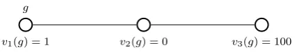
v1(g) = 1 g
[image:16.595.192.406.110.148.2]v2(g) = 0 v3(g) = 100
Figure 1: Low global efficiency despite high clique-wise efficiency
Observe thatAandA0 are clique-variants of each other if and only ifδ= (A, A0) is a clique-deal.
Definition 8(Clique-wise efficiency). An allocationAis called clique-wise efficient ifsw(A)>sw(A0) for every clique-variantA0 of A.
It should be noted that, in its own right, this notion of efficiency would only be of very limited inter-est. In particular, as the following example demonstrates, an allocation that is clique-wise efficient can be arbitrarily bad in terms of global efficiency. Consider Figure 1, showing a negotiation topology between three agents, together with the valuation each of these three agents assigns to the goodg. Now suppose that in allocationA, itemg is assigned to agent 1, i.e., social welfare is 1. The only clique-variant ofA is the allocation whereg is given to agent 2, which would reduce social welfare to 0. Thus,A is clique-wise efficient. On the other hand, allocation A0, giving g to agent 3 instead, would increase social welfare by a factor of 100.
The reader might doubt the significance of this example and point out that the chosen valuation functions are extremely different from each other, or that a line topology might be a particularly problematic case to handle. But in fact, this kind of situation can occur also under much more favourable circumstances, as the following result shows:
Proposition 12 (Global inefficiency of clique-wise efficiency). If the negotiation topology is not complete, then the social welfare of a clique-wise efficient allocation can be arbitrarily far from the optimum. This holds even when all agents share the same single-minded valuation function.
Proof. LetG= (N, E) be a graph that is missing at least one edge. W.l.o.g., assume that agent 1 is not connected to agent 2. Let the set of goods be {g1, g2}. Assume all agents share the same single-minded
valuation functionvwithv({g1, g2}) = 1 andv(S) = 0 for all bundlesS6={g1, g2}. Consider the allocationA
in which agent 1 ownsg1 and agent 2 ownsg2. In allocationA, if no payments have been made in the past,
the utility of every agent is equal to 0, and thus so is social welfare. Nevertheless,Ais clique-wise efficient, because any clique ofGmust be a subset of either{1,3,4, . . . , n}or{2,3,4, . . . , n}, i.e., no clique collectively owns bothg1andg2. On the other hand, any allocation where one agent owns both items has a social welfare
of 1. Thus, the ratio between the social welfare of efficient allocations and the social welfare of clique-wise efficient allocations cannot be bounded by a constant.
This result may call into question the usefulness of Definition 8. While our definition of envy with respect to a graph is very natural and reaching GEF states seems indeed desirable, it is questionable whether it is at all possible to relativise the standard notion of efficiency with respect to a negotiation topology in a meaningful manner. Our interest in the purely technical definition of clique-wise efficiency given above stems from the fact that it will be helpful in characterising conditions under which convergence to a GEF state can be guaranteed (as will become clear in the sequel). But first we prove a convergence result for clique-wise efficiency:
Lemma 13 (Clique-wise efficient outcomes). Any sequence of IR clique-deals will eventually result in a clique-wise efficient allocation of goods.
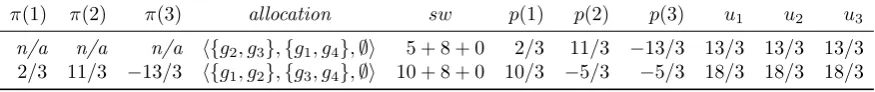
π(1) π(2) π(3) allocation sw p(1) p(2) p(3) u1 u2 u3
n/a n/a n/a h{g2, g3},{g1, g4},∅i 5 + 8 + 0 2/3 11/3 −13/3 13/3 13/3 13/3
[image:17.595.79.517.113.159.2]2/3 11/3 −13/3 h{g1, g2},{g3, g4},∅i 10 + 8 + 0 10/3 −5/3 −5/3 18/3 18/3 18/3
Table 4: Convergence via deals between neighbouring agents 1 and 2
Lemma 13 generalises Theorem 1. The latter corresponds to the case of a fully connected graph. While Lemma 13 guarantees clique-efficient outcomes, it does not say anything aboutwhichclique-efficient alloca-tion will be reached. For most graphs there will be a range of clique-efficient allocaalloca-tion of varying quality in terms of global efficiency (in this sense the concept is similar to that of Pareto efficiency). There is no guar-antee that we will end up with the “best” clique-efficient allocation. And even if it does, as Proposition 12 shows, global efficiency may still be arbitrarily bad. Nevertheless, as we will see next, clique-wise efficiency is a sufficiently strong notion to serve as a basis for negotiating envy-free states.
5.3. Convergence
We now prove a convergence theorem for GEF states, which extends Theorem 8 to the framework with a negotiation topology: we show that under the same conditions (on the valuation functions and for a particular choice of payment scheme), any sequence of IR deals that respect the negotiation topology will result in a GEF state.
Theorem 14(Convergence on graphs). If all valuations are supermodular and if initial equitability payments have been made, then any sequence of IR clique-deals using the GUPF will eventually result in a GEF state.
Proof. Recall from the proof of Theorem 8 that the use of the GUPF together with initial equitability payments ensures that we get a payment balance satisfyingπ(i) = vi(A)−sw(A)/n for every state (A, π)
reached during negotiation and every agent i ∈ N. By Lemma 13, negotiation will eventually terminate and the final allocation A∗ will be clique-wise efficient. The associated payment balance will be π∗(i) = vi(A∗)−sw(A∗)/n. We need to show that the state (A∗, π∗) must be GEF whenever all valuationsvi are
supermodular. Letiandjbe any two agents. Ificannot seejthen we are done. Otherwise,iandjare part of a clique, and due to the clique-wise efficiency ofA∗, giving bothA∗(i) and A∗(j) to iwill not increase the sum of valuations for this clique any further. Hence, by the argument familiar from Section 4.1,idoes not envyj in state (A∗, π∗).
Theorem 14 means that agents can negotiate in a distributed manner, guided only by their own rational interests and limited to their “neighbourhoods” as given by the cliques of the negotiation topology, and—as long as all the side conditions are satisfied—a state that is envy-free according to all agents (whose vision is limited by the negotiation topology) will eventually emerge. In particular, agents can go ahead and negotiate any beneficial deals, without fear of getting stuck in a local optimum.
Example 4. We consider once more the allocation problem of Table 1, but now the agents are arranged on a line, with agent 1 in the middle position, i.e.,E={(1,2),(2,1),(1,3),(3,1)}. Suppose the initial allocation isA0 =h{g2, g3},{g1, g4},∅i. Table 4 shows the allocations visited during a sequence consisting of a single
IR clique-deal, which culminates in a clique-wise efficient state(A0, π0), in which the final payment balances of the agents are as follows: π0(1) = 12/3,π0(2) = 6/3, andπ0(3) =−18/3. The final utility of each agent is18/3. It can be checked that the following statements hold.
• Agent 2 does not envy agent 1, as u2(A0(1), π0(1)) = 8−12/3 = 12/3<18/3
• Agent 3 does not envy agent 1, as u3(A0(1), π0(1)) = 0−12/3 =−12/3<18/3
• Agent 1 does not envy agent 2 nor agent 3, as both:
– u1(A0(3), π0(3)) = 0 + 18/3 = 18/3
Thus, no agent envies any of her neighbours. However, note that if agent 3 could see agent 2, envy would occur asu3(A0(2), π0(2)) = 10−6/3 = 24/3>18/3.
A critical point in Theorem 14 is the use of the GUPF, as this payment function does not respect the negotiation topology. However, it is easy to show that there can be no clique-wise payment function (a payment function giving non-zero payments only to agents belonging to a particular maximal clique within which the deal is taking place) that would allow us to achieve a convergence result for GEF states. To see this, consider the following example. Suppose again there are three agents on a line, the payment balance is currently 0 for all agents, and the valuation function of agent 3 isv3(S) = 0 for anyS ⊆ G. Then any
deal between agents 1 and 2, where the former makes a non-zero payment to the latter, will render agent 3 envious of agent 2.
A variation of this example shows that even when there exists a clique-wise payment function leading to a GEF state, the exact amount of the payments to be made may depend on agents outside the clique where the deal is taking place. For the same negotiation topology as above, let againv3(S) = 0 for any S ⊆ G,
but now suppose that agent 3 has benefited from a previous deal in monetary terms, i.e.,π(3) =xfor some x <0. Then an envy-eliminating deal between agents 1 and 2 should be such that it brings the payment balance of agent 2 to at least xas well (which may or may not be possible, depending on the scenario at hand). This shows that the best possible clique-wise payment function may not be identifiable locally.
A positive point to be made about the GUPF is that the payments to non-involved agents (in particular those outside the clique where the deal is taking place) solely depend on the social surplus generated by the deal and the overall number of agents in the system. So agents do only need to be “aware” of agents they cannot “see” in so far as they need to know their overall number. This arguably corresponds well to human society: our sphere of influence may be very much restricted to a small section of society defined by the social network we belong to, but we are still aware of some basic facts concerning society as a whole (such as the number of its members).
Finally, in analogy to Theorems 5 and 11, if all valuation functions are modular, then we can strengthen Theorem 14 and prove convergence by means of IR 1-deals between connected agents using our by now familiar technique.
Theorem 15 (GEF outcomes by 1-deals). If all valuation functions are modular and if initial equitability payments have been made, then any sequence of IR 1-deals between pairs of connected agents using the GUPF will eventually result in a GEF state.
5.4. Path length
Just as we did for Theorems 4 and 8, also for Theorem 14 we may ask how many deals are required before the system converges. Now the bounds on the longest (as well as the shortest) path will depend on the negotiation topology. At one extreme, if the graph is fully connected then Theorem 14 reduces to Theorem 8 and we obtain the same bounds as before. In particular,nm−1 will always be an upper bound on the longest
path. At the other extreme, if no two agents are connected to each other, then no deals are possible, and the upper bound reduces to 0. In general, it is clear that the sparser the graph, the shorter the longest path to convergence we can construct. The question now arises whether there is a class of graphs that is relatively sparse (but still natural and attractive for applications) that would result in a significant reduction of the length of the longest possible path. The answer to this question, unfortunately, is negative. As we will see next, even if agents are arranged on a line (a highly simplistic negotiation topology), there may still be a number of IR deals that is exponential in the number of goods.
Proposition 16 (Path length for line topology). Suppose the negotiation topology G= (N, E) is a line: E={(i, j)∈ N2| |i−j|= 1}. Then we can find a valuation function for each agent such that there exists
Proof. Suppose the agents have the valuation functions defined in the proof of Lemma 6 and initially allocate all goods to agent 1. Then agents 1 and 2 can go through all 2m allocations that divide all goods between
the two of them and end up in the allocation where agent 2 owns all items (that is, there are 2m−1 IR
deals between them). We can do the same for every one of then−1 pairs (i, i+ 1) of connected agents and thus end up with a path of the claimed length of (2m−1)·(n−1) deals.
Note that our construction is independent of the payment scheme used. In particular, it applies in case the payment scheme of Theorem 14 is in operation.
Interestingly, the upper bound of the shortest path may increase as the graph connecting the agents becomes sparser, simply because this means that some transactions cannot be executed as a single deal anymore. For the scenario described in the proof of Proposition 16 the shortest path would ben−1 (rather than 1, the bound for fully connected graphs): we can reach the social optimum by implementing one deal per pair of neighbouring agents.
6. Degrees of envy and computational complexity
The convergence theorems of the previous two sections show that envy-freeness can be guaranteed for the outcome of a distributed negotiation process, under specific assumptions. But this is certainly not the final word on the matter. The payment scheme used in these theorems introduces a non-local element, in the sense that it redistributes the social surplus over the whole of society. One may ask how a local payment function, such as the LUPF, would fare in comparison. Also, one could object to the requirement that initial payments have to be made. The restriction to supermodular valuation functions in Theorems 8 and 14 is another limitation. Lastly, our convergence theorems do not say how envy evolves over the course of negotiation. Because negotiation can become very long in practice, it is possible that the process will have to be stopped before completion. In that event, it would be valuable to be able to guarantee some monotonicity properties—but with respect to what parameter?
To be able to address such questions, more than the mere classification of a negotiation state as being either envy-free or not is needed. We require a way to measure thedegree of envyin a society. In this section, we will propose a systematic approach to defining measures for assessing the degree of envy. We propose to analyse the degree of envy of a society as a three-level aggregation process, starting with envy between two agents, over envy of a single agent towards everyone else, to eventually provide a definition for the degree of envy of a society. We also formulate a number of fundamental axioms that any reasonable measure of envy, not only the concrete measures proposed here, should satisfy. Towards the end of the section we then prove a theorem on the computational complexity of the problem of finding an IR deal that reduces envy according to any such measure.
6.1. Envy between two individual agents
How much does agentienvy agentj in state (A, π)? Any measure of envy betweeniandj will be based on ∆i,j(A, π) =ui(A(j), π(j))−ui(A(i), π(i)), the difference in utility that iassigns to their own lot and that
ofj. If this number is negative or equal to 0, then agentidoes not envy agentj, nor does she in case she cannot see agentj in the social network. This gives rise to a matrix of dimensionn×n, with entriesei,j:
ei,j =
∆i,j(A, π) if ∆i,j(A, π)>0 and (i, j)∈E
0 otherwise
We now useei,j to define two different measures for the degree of envy between individual agents:
eraw(i, j) = ei,j ebool(i, j) =
1 ifei,j >0
0 otherwise
The second measure (ebool) only allows us to specify whether or notienviesj. In many cases this is all that is needed. The first measure is useful if we also want to say how much i enviesj. In principle one could also consider the notion of “negative envy” [1], i.e., one could consider treating the case of ∆i,j(A, π)<0