MoL 2012 15: Automatic Verication of Programs with Indirection

Automatic Verification of Programs with Indirection

MSc Thesis

(Afstudeerscriptie)

Kyndylan Nienhuis

(born February 10th, 1989 in Amsterdam, The Netherlands)

under the supervision of Prof Dr Jan van Eijck, and submitted to the Board of Examiners in partial fulfillment of the requirements for the degree of

MSc in Logic

at theUniversiteit van Amsterdam.

Date of the public defense: Members of the Thesis Committee: September 4th, 2012 Prof Dr Jan van Eijck

Abstract

In the first part we prove the correctness of an existing verification algorithm, namely counterexample-driven abstraction refinement. To be able to state the correctness of the algorithm, we modify it such that it verifies programs that have a formal semantics. We use propositional dynamic logic and we give a denotational semantics and an equivalent structural operational semantics.

Then we consider a deterministic fragment of propositional dynamic logic. We improve the efficiency of the algorithm by exploiting determinism when present and we prove that this algorithm terminates on incorrect determinis-tic programs. Note that the algorithm will not always terminate on correct deterministic programs, since verification is undecidable in general.

Acknowledgements

Contents

1 Introduction 2

1.1 Automatic verification . . . 2

1.2 Overview . . . 3

2 Propositional dynamic logic 5 2.1 Language . . . 5

2.2 Semantics . . . 6

2.3 A non-deterministic boolean model . . . 7

3 Control flow graphs 11 3.1 Language and semantics . . . 11

3.2 Connection with propositional dynamic logic . . . 12

3.3 Equivalence of semantics . . . 15

4 Abstraction refinement 20 4.1 Overview . . . 20

4.2 Assumptions . . . 22

4.3 Abstractions . . . 23

4.4 Path constraints . . . 26

4.5 Refinements . . . 26

4.6 Correctness . . . 30

5 Deterministic propositional dynamic logic 32 5.1 Language and semantics . . . 32

5.2 Determinism . . . 36

5.3 Partition refinement on D-PDL . . . 38

5.4 Termination . . . 42

5.5 Verification of the lock/unlock example . . . 43

6 Indirection 47 6.1 Language . . . 47

6.2 Path constraints . . . 48

6.3 Symbolic execution . . . 49

6.4 Correctness . . . 51

Chapter 1

Introduction

A specification of a computer program is a formal description of the properties that we want the program to have. Verifying a program means checking whether the program satisfies the properties in its specification.

We start with an example. Consider the program in Listing 1.1 on the fol-lowing page. This program waits until a message is available and then processes the message. Other programs can also manipulate the messages, therefore there is a lock that a program has to hold when accessing or changing the messages. The program in Listing 1.1 acquires a lock while checking for a message, retriev-ing the message and processretriev-ing the message. If there is no message available it releases the lock to allow other programs to make a message available.

We want that the program uses the lock in a correct way. Constructing a specification that precisely describes what we think is the correct way is not in the scope of this thesis. For this program we take the following property as its specification which captures at least a part of what it means to use the lock in a correct way.

“The program does not calllockwhen it has the lock, orunlock

when it does not have the lock.”

To see that the example program satisfies this specification, observe that at the end of the loop we have has messages = trueif and only if the program has the lock.

1.1

Automatic verification

Listing 1.1 A program that callslockandunlockin alternation

//Acquire message has messages = false; while (not has messages) {

lock();

has messages = check messages(); if (has messages) {

message = get message();

}

else {

unlock(); sleep();

} }

//Process message do stuff(message); .

. .

do stuff(message); unlock();

programs. Both methods have successfully been used to find bugs, but they can only prove a program correct by exhaustively checking all states.

Cousot and Cousot [6] introduced abstraction techniques that can be used to check multiple states at once. When essential details are abstracted away, verifying an abstraction has the possibility to lead to wrong results. To keep the error one-sided Clarke, Grumberg and Long [5] defined overapproximations that do not allow false positives. In [4] Clarke et al. showed how false negatives can be used to refine an overapproximation. This is called counterexample-driven refinement.

Counterexample-driven refinement has been implemented in the tool Yogi [1] that has been used to efficiently verify windows device drivers. In this al-gorithm the initial abstraction abstracts away from everything and only details are included that are necessary to avoid false negatives.

1.2

Overview

We restrict ourselves to partial correctness specifications. A partial correctness specification is a triple ϕpre{α}ϕpost where α is a formal program and ϕpre and ϕpost conditions on the program. It states that whenever α is executed in a state where ϕpre holds, then ϕpost holds in every state that could be the result of executingα. This form of specifying was proposed by Floyd and Hoare [8, 10].

In Chapter 2 we introduce the framework we use to describe programs and specifications. We have chosen propositional dynamic logic (PDL) because it can express partial correctness specifications in a very simple and elegant way. We translate the program in 1.1 and its specification to PDL.

graphs and we connect this with propositional dynamic logic.

Then in Chapter 4 we define the abstraction refinement algorithm that can verify propositional dynamic logic programs. We use overapproximations and counterexample-driven refinement as described before and we prove the correct-ness of this algorithm.

In Chapter 5 we consider a fragment of PDL that has deterministic code constructs and allows for deterministic and non-deterministic actions. We adapt the abstraction refinement algorithm such that it exploits the fact that some actions are deterministic. We prove that when all actions are deterministic, the algorithm will eventually terminate on programs that are incorrect. Note that this result cannot be extended to all correct or incorrect, deterministic programs, since verification is undecidable. We conclude this chapter by running the abstraction refinement algorithm on the PDL version of the program given in Listing 1.1.

Chapter 2

Propositional dynamic logic

Propositional dynamic logic was developed by Pratt [14] and Fischer and Ladner [7]. In this thesis we will use the definition of Fischer and Ladner. PDL has a complete axiomatization, see for example [13].

For an introduction to propositional dynamic logic and an overview of its uses we recommend [16]. PDL is a multimodal logic, see [2] for a thorough introduction to modal logic.

We will define the language of propositional dynamic logic in Section 2.1, its semantics in Section 2.2 and in Section 2.3 we define a model that is able to capture the essence of the program described in Listing 1.1 on page 3.

2.1

Language

The language of propositional dynamic logic consists of formulas and programs. It is parametrized by a signature to be able to describe various other languages.

Definition 2.1 (Signature). A signature is a pair (P,B) withP a set of propo-sitions andBa set of basic actions.

Definition 2.2(Formulas and programs). With simultaneous recursion we de-fine the set Φ of formulas and the set Π of programs over the signature (P,B). Letp∈ P, b∈ B, ϕ1, ϕ2∈Φ andα1, α2∈Π, then

ϕ ::= > |p| ¬ϕ1|ϕ1∧ϕ2| hα1iϕ1

α ::= b|?ϕ1|α1;α2|α1∪α2|α∗1.

The intended meaning ofhαiϕis that there exists a computation of αthat results in a state where ϕis the case. The connection between propositional dynamic logic and modal logic is thathαican be seen as a modal operator.

The base cases in the definition of programs are programs of the formbor ?ϕ. The former is a basic action and the latter a test action, that tests whether ϕholds.

Programs can be composed in three ways: α1;α2 is the sequential

compo-sition of α1 and α2,α1∪α2 is the program that non-deterministically chooses

betweenα1andα2andα∗ is the program that executesαan arbitrary number

We use the following abbreviations

⊥ = ¬>

ϕ∨ψ = ¬(¬ϕ∧ ¬ψ) ϕ→ψ = ¬ϕ∨ψ

ϕ↔ψ = (ϕ→ψ)∧(ψ→ϕ)

[α]ϕ = ¬hαi¬ϕ.

Given the intended meaning ofhαi, we see that [α]ϕ=¬hαi¬ϕmeans that in every state that is a result of the execution ofαwe have thatϕholds.

The modal operator hαi enables us to express a partial correctness speci-fication ϕpre{α}ϕpost. We have no need to allow program modalities in the conditionsϕpre andϕpost, thus we use the following definition.

Definition 2.3 (Specifications). A partial correctness specification of a pro-gram α is a pair (ϕpre, ϕpost) ∈ Φ×Φ where ϕpre and ϕpost do not contain program modalities. Furthermore, we require that every test action ?χ in α also does not contain program modalities. The propositional dynamic logic formula that states thatαis correct isϕpre→[α]ϕpost.

2.2

Semantics

We define the semantics over a labeled transition system where labels are actions b∈ B. This is a generalization of a Kripke structure that is used as a model for modal logic.

Definition 2.4 (Models). A model over the signature (P,B) is a tupleM = (Σ,V,R) where Σ is a set of states, V a valuation that sendsp∈ P to the set

V(p)⊆Σ wherepis true andRa function from labels to transitions that sends b∈ Bto the binary relationR(b)⊆Σ×Σ.

The binary relation R(b) describes the meaning of the basic action b as follows. We say (s, r)∈ R(b) when ris a possible resulting state of executing b in the states. When there are multiple r∈Σ with (s, r)∈ R(b) then b is a non-deterministic action. When there is nor∈Σ with (s, r)∈ R(b) the action b cannot be executed ins.

The interpretation of a programαwill be a binary relation with the same meaning. Before we can define this, we need the following general definitions about binary relations.

Definition 2.5. LetR1andR2be binary relations over a setS. The relational

composition is defined as

R1◦R2={(s1, s3)∈S×S| ∃s2∈S(s1, s2)∈R1∧(s2, s3)∈R2}.

Then-fold composition of a relationR with itself is recursively defined

R0 = {(s, s)|s∈S}

The reflexive transitive closure ofRis given by

R∗=

∞

[

i=0

Ri.

Definition 2.6(Semantics). The interpretation of a formulaϕ∈Φ in a model M = (Σ,V,R) is a set of statesIM_{(ϕ)⊆Σ whereϕis true and the} interpreta-tion of a programα∈Π is a binary relationIM_{(α)⊆Σ×Σ. We defineI}M _by simultaneous recursion.

IM_{(>) = Σ}

IM_{(p) = V(p)}

IM_(¬ϕ

1) = Σ− IM(ϕ1)

IM_(ϕ

1∧ϕ2) = IM(ϕ1)∩ IM(ϕ2)

IM_(hα

1iϕ1) = s∈Σ| ∃t∈Σ (s, t)∈ IM(α1)∧t∈ IM(ϕ1) .

IM_{(b) = R(b)}

IM_{(?ϕ) =}

(s, s)∈Σ×Σ|s∈ IM_(ϕ)

IM_(α

1;α2) = IM(α1)◦ IM(α2)

IM_(α

1∪α2) = IM(α1)∪ IM(α2)

IM_(α∗

1) = I

M_(α

1)

∗

.

The binary relationIM_{(α) describes the programαby specifying every pair} (s, r) of states such thatris a possible end state whenαis executed in the state s.

We writeM, s ϕfor s∈ IM_{(ϕ). When M is clear from the context, we} abbreviateM, sϕtosϕ. We say M ϕif for alls∈Σ we havesϕ.

Definition 2.7 (Verification). Let (ϕpre, ϕpost) be a specification of the pro-gramα. Verifyingαagainst this specification is deciding whetherM ϕpre→ [α]ϕpost orM 2ϕpre→[α]ϕpost.

2.3

A non-deterministic boolean model

We define a model that serves as an example of the framework we defined in this chapter and that can be used to describe the program of Listing 1.1 on page 3. The language consists of boolean variables and deterministic and non-deterministic assignments. We will call this model NDB.

Letbool={>,⊥}. Define the signature (P,B) whereP is a set of variables and

B={p:=random|p∈ P} ∪ {p:=x|p∈ P, x∈bool}.

We take the model M = (Σ,V,R) where Σ is the set of functions from P to bool,

V(p) = {s∈Σ|s(p) =>},

(s, r) ∈ R(p:=random) iffs(q) =r(q) for all q6=p,

Example 2.8. Consider the program defined in Listing 1.1 on page 3. We will describe this program in NDB. We use the three variableslock, has mandf oo. The first denotes whether the lock has been acquired or not, the second whether there is a message to process and the last to do irrelevant calculations with.

Every time the functioncheck messages()is called in the program, it can returntrue andfalsearbitrarily. Hence, we model it using a random assign-ment. We also model the irrelevant computations with random assignments, because we do not care about what happens. The translation of the statements is thus as follows

lock() 7→ lock:=>

unlock() 7→ lock:=⊥

has messages = false 7→ has m:=⊥

has messages = check messages() 7→ has m:=random

message = get message() 7→ f oo:=random

sleep() 7→ f oo:=random

do stuff(message) 7→ f oo:=random.

We model the control flow statements as follows, see Chapter 5 for the intuition behind this choice of modeling.

if (ϕ){α1} else {α2} 7→ (?ϕ;α1)∪(?¬ϕ;α2)

while (ϕ) {α} 7→ (?ϕ;α)∗; ?¬ϕ.

The translated program is given in Figure 2.1 on the following page. As stated in the introduction the specification we want to check is “The program does not calllock when it has the lock, orunlockwhen it does not have the lock.” To model this in our framework we introduce a new variable error. We replace the following calls

lock:=> 7→ (?lock;error:=>)∪(?¬lock;lock:=>) lock:=⊥ 7→ (?lock;lock:=⊥)∪(?¬lock;error:=>).

Listing 2.1 Lock/unlock program in NDB

has m := ⊥; (

? ¬has m; lock := >; has m := random; (

? has m; foo := random

∪

? ¬has m; lock := ⊥; foo := random )

Listing 2.2 Lock/unlock program with error check

has m := ⊥; (

? ¬has m; (

? lock; error := > ∪

? ¬lock; lock := >

);

has m := random; (

? has m; foo := random

∪

? ¬has m; (

? lock; lock := ⊥ ∪

? ¬lock; error := >

);

foo := random )

)*; ? has m; foo := random; (

? lock; lock := ⊥ ∪

? ¬lock; error := >

Chapter 3

Control flow graphs

While propositional dynamic logic makes it easy to describe a program and its specification, the recursive definition of programs makes it difficult to prove or disprove that a program satisfies its specification. To overcome this we will in-troduce semantics that describes all the individual steps of executing a program. From now on, we will call the semanticsI defined in the previous chapter the denotational semantics and use the notationIds. The semantics defined in this

chapter is called the structural operational semantics, it is denoted byIsos. See

[12] for a comparison between different styles of defining semantics.

We will use control flow graphs to define the structural operational semantics. Control flow graphs have a language and models of its own, to avoid confusion we will call the signatures and models defined in the previous chapter PDL-signatures and PDL-models and the signature and models of control flow graphs CFG-signatures and CFG-models. In later chapters we will not be concerned with CFG-signatures and CFG-models anymore, and then we will drop the prefix PDL. The notation for the semantics of control flow graphs isIgraph.

In Section 3.1 we define control flow graphs, CFG-models and the interpre-tation Igraph. In the next section we will define a translation from programs

to control flow graphs and use this to define the structural operational seman-tics Isos. Then in Section 3.3 we will prove that the structural operational and

denotational semantics are equivalent.

3.1

Language and semantics

The language of control flow graphs is parametrized by a set of actions. When we make the connection with PDL, this set will differ from the setBin a PDL-signature (P,B). Hence, we define CFG-signatures separately.

Definition 3.1 (CFG-signature). A CFG-signature is a setAof actions.

Definition 3.2(Control flow graphs). A control flow graphGoverAis a tuple (N, I, F, E) where N is a finite set of nodes, I, F ∈N are its initial and final nodes andE⊆N× A ×N a set of directed, labeled edges.

We will use the following notation for a path γ that traverses the nodes g0, . . . , gn along edges labeled with the actions a1, . . . , an

γ=g0

a1

→g1

a2

→. . .an

→gn.

CFG-models have exactly the same structure as PDL-models, except that there is no need for a valuation function V. Since A can differ from the set

B, we cannot simply use the relevant aspects of a PDL-model and we need to define CFG-models separately.

Definition 3.3(CFG-models). A CFG-modelKover the signatureAis a tuple (Σ,R) where Σ is a set of states andRa function that mapsa∈ Ato the binary relationR(a)⊆Σ×Σ.

We have said that nodes represent stages during a computation and outgo-ing edges the possible next actions. A path in a control flow graph therefore represents a part of the computation. We use the word trace as a synonym for a finite sequence of states. We define the connection between traces and paths in the control flow graph as follows.

Definition 3.4 (Satisfying traces). Letγ be a path of length nin the control flow graph G, leta1, . . . , an be the labels of the edges. We say that the trace s0, . . . , sn of lengthn+ 1 withsi ∈Σ satisfiesγif for alli∈ {1, . . . , n} we have (si−1, si)∈ R(ai).

The possible paths inGthat start at the initial nodeI and end at the final nodeF define the program thatGrepresents.

Definition 3.5 (Semantics). The interpretation of a control flow graph Gin the CFG-model K is a binary relation IK

graph(G) ⊆ Σ×Σ. It is defined by

(s, r)∈ IK

graph(G) iff there is a pathγ in Gthat starts atI and ends atF and

a trace (s, t1, . . . , tn−1, r) that satisfies γ.

3.2

Connection with propositional dynamic logic

We will use control flow graphs to represent PDL programs. We have defined control flow graphs over a set Aof actions. Since programs can contain basic actionsb∈ Band test actions ?ϕ, we translate a PDL-signature (P,B) therefore to the CFG-signatureA=B ∪ {?ϕ|ϕ∈Φ}that is the union of basic and test actions.

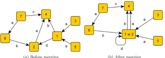
Before we define the translation from programsα∈Π to control flow graphs, we define how to merge two nodes in an arbitrary graph. See Figure 3.1 on the next page for an example.

Definition 3.6 (Merging nodes). LetG be a graph with nodesN and edges E⊆N× A ×N and letg0, g1∈N be the nodes that will be merged. We define

(a) Before merging (b) After merging

Figure 3.1: Merging the nodes 1 and 2

Letg be a new node, we writeg=g0]g1. The set of nodes ofG0 is given

by

N0=N∪ {g}\{g0, g1}.

We do not want to change anything essential about the edges. So if g0 or

g1 is part of an edge in G, then g will have the same role in an edge in G0.

Formally, we defineE0 as follows

E0 = E∩(N0× A ×N0)

∪ {(h, a, g)|a∈ A, h∈N0(h, a, g0)∈E or (h, a, g1)∈E}

∪ {(g, a, h)|a∈ A, h∈N0(g0, a, h)∈E or (g1, a, h)∈E}

∪ {(g, a, g)|a∈ Aif there arex, y∈ {g0, g1}with (x, a, y)∈E}.

We can now define the translation from PDL programs to control flow graphs.

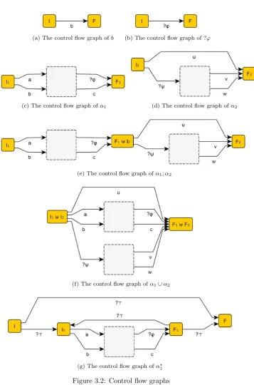
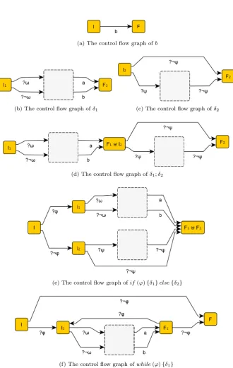
Definition 3.7. Let α ∈ Π be a program. We define its control flow graph G(α) with induction to the structure ofα. See Figure 3.2 on the following page for an illustration.

Case1. Base cases: α=aorα=?ϕ. DefineGas the graph with two nodes I and F; and an edge from I to F labeled with the (basic or test) actionα.

Case2. Recursive cases. Let G1 and G2 be the control flow graphs of α1

andα2respectively and letI1,I2andF1, F2 denote their respective

initial and final nodes.

Case i. α=α1;α2. First defineGas the disjoint union ofG1 and

G2. Set I=I1 and F =F2 and merge the node F1 with

I2.

Case ii. α= α1∪α2. First define Gas the disjoint union of G1

and G2. Set I = I1 and F =F1 and merge the node I1

withI2andF1 withF2.

Case iii. α=α∗₁. DefineGas the disjoint union ofG1with two new

nodesI andF. Add the following edgesI →I1,I →F,

(a) The control flow graph ofb (b) The control flow graph of ?ϕ

(c) The control flow graph ofα1 (d) The control flow graph ofα2

(e) The control flow graph ofα1;α2

(f) The control flow graph ofα1∪α2

(g) The control flow graph ofα∗1

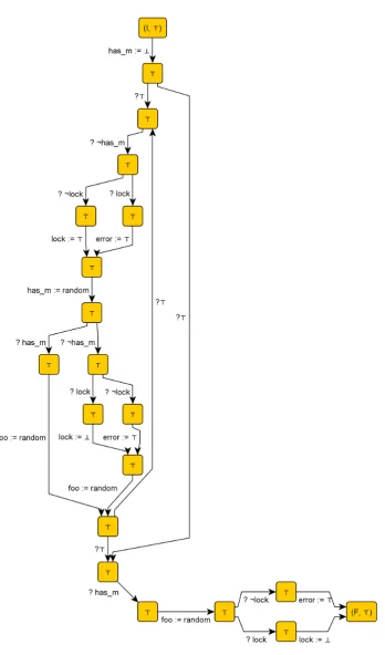
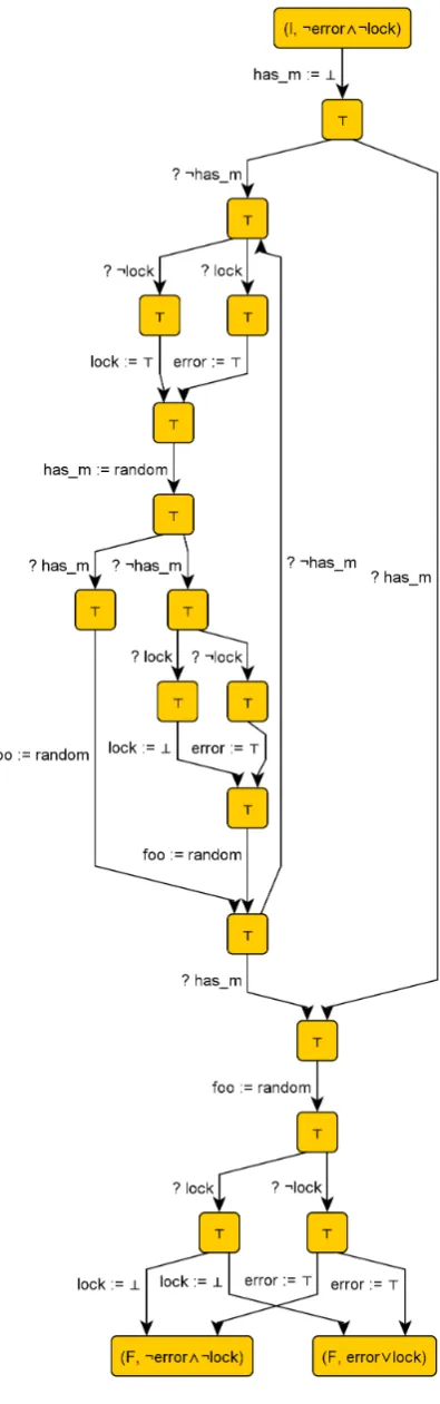
Example 3.8. Recall the lock/unlock program defined in Listing 2.2 on page 10. In Figure 3.3 on the following page its control flow graph is shown.

From Figure 3.2 on the previous page we can make the following observation. We will need this detail when defining the verification algorithm.

Fact 3.9. Let α be a program, there does not exist a node in the control flow graph G(α)that has an edge to itself.

Now we are ready to define the structural operational semantics. Since pro-grams can contain formulas as test actions and formulas can contain propro-grams in modalities, the interpretation of formulas and the interpretation of programs depend on each other. We will let the structural operational interpretationIsos

of programs depend on the denotational interpretationIdsof formulas. The

de-notational interpretation of formulas is however dependent on the dede-notational interpretation of programs, so indirectly the definition of Isos of programs

de-pends on the definition ofIds of programs.

This apparent dependency disappears when we have proven thatIsos(α) =

Ids(α). Then the structural operational interpretation of programs can be seen

on its own right.

Definition 3.10(Structural operational semantics). LetM = ΣM_,VM_,RM

be a PDL-model. The interpretation a program α ∈ Π is a binary relation

IM

sos(α)⊆ΣM ×ΣM. Define the CFG-model K= ΣK,RK

where ΣK _{= Σ}M and

RK_{(a) =}

(

RM_{(b) ifa=b∈ B}

(s, s)|s∈ IM

ds(ϕ) ifa=?ϕ, ϕ∈Φ.

Then define

IsosM(α) =I

K

graph(G(α)).

3.3

Equivalence of semantics

The proof that IM

sos(α) = IdsM(α) will be with induction to the structure of α.

We will first prove the base case.

Lemma 3.11. LetM = ΣM,VM_,RM

be a PDL-model. Leta∈ Abe a basic or test action, we haveIM

sos(a) =IdsM(a).

Proof. Let K = ΣK_,RK

be the CFG-model as defined in Definition 3.10. We have IM

sos(a) = IgraphK (G(a)). The control flow graph G(a) is the graph

I → F where the edge is labeled with a, see Definition 3.7 on page 13. Since there is only one path from Ito F, we have (s, r)∈ IK

graph(G(a)) if and only if

(s, r)∈ RK_(a).

Case1. a = b with b ∈ B. By definition, RK_{(b) = R}M_{(b) and I}M

ds(b) =

RM_{(b). HenceI}M

sos(b) =IdsM(b).

Case2. a=?ϕwithϕ∈Φ. By definition

RK_{(?ϕ) =}

(s, s)∈Σ×Σ|s∈ IM

ds(ϕ)

which is the same as the definition of IM

ds(?ϕ). Hence, IsosM(?ϕ) =

IM

To clean up the notation, we now fix a modelM = (Σ,V,R) and we omit the superscriptM in IM

ds andIsosM.

Recall from Definition 2.6 on page 7 that the recursive cases of the definition ofIds are given by

Ids(α1;α2) = Ids(α1)◦ Ids(α2)

Ids(α1∪α2) = Ids(α1)∪ Ids(α2)

Ids(α∗1) = (Ids(α1))∗.

For each of these cases, we will prove a lemma that states thatIsos behaves

in the same way.

Lemma 3.12. We haveIsos(α1;α2) =Isos(α1)◦ Isos(α2).

Proof. The idea is that paths inG(α1;α2) can be split into a path inG(α1) and

a path inG(α2). Vice versa, a pathγ1 inG(α1) and a pathγ2 inG(α2) can be

concatenated to form a path inG(α1;α2), see Figure 3.2e on page 14.

Suppose (s1, s3)∈ Isos(α1;α2). Then there is a path γ in the control flow

graph of α1;α2 and a traceσfroms1 tos3 that satisfiesγ.

γ = I a1

→g1

a2

→. . .a→n−1gn−1

an

→F

σ = (t0, . . . , tn) witht0=s1, tn=s3.

This path has to crossF1]I2 somewhere, see Figure 3.2e on page 14, leti

be the index such thatgi=F1]I2. Define the pathsγ1,γ2 and the tracesσ1,

σ2

γ1 = I1

a1

→g1

a2

→. . .a→i−1gi−1

ai

→F1

γ2 = I2

ai+1

→ gi+1

ai+2

→ . . .a→n−1gn−1

an

→F2

σ1 = (t0, . . . , ti) σ2 = (ti, . . . , tn).

We have thatγ1is a path in the control flow graph ofα1andγ2in the control

flow graph of α2. Furthermore, σ1 satisfies γ1 and σ2 satisfies γ2. Hence, we

have (t0, ti) ∈ Isos(α1) and (ti, tn) ∈ Isos(α2). We conclude that (t0, tn) ∈

Isos(α1)◦ Isos(α2).

For the other direction, suppose (s1, s3)∈ Isos(α1)◦ Isos(α2). Then there

is a s2 with (s1, s2)∈ Isos(α1) and (s2, s3)∈ Isos(α2). Hence, there are paths

γ1 and γ2 in the control flow graphs of respectively α1 and α2 with satisfying

tracesσ1 andσ2.

γ1 = I1

a1

→g1

a2

→. . .a→n−1gn−1

an

→F1

γ2 = I2

b1

→h1

b2

→. . .bk→−1hk−1

bk

→F2

σ1 = (r0, . . . , rn) withr0=s1, rn=s2

These paths can be concatenated to the pathγin the control graph ofα1;α2

and these traces can be combined to σas follows. Note that when combining σ1andσ2 toσwe omittedt0.

γ = I a1

→g1. . . gn−1

an

→F1]I2

b1

→h1. . . hk−1

bk

→F

σ = (r0, . . . , rn, t1. . . , tk).

Sincern =t0 we have thatσsatisfiesγ. Sincer0=s1and tk =s3 we have

(s1, s3)∈ Isos(α1;α2).

Lemma 3.13. We haveIsos(α1∪α2) =Isos(α1)∪ Isos(α2).

Proof. From Figure 3.2f on page 14 it follows that every path γ in the control flow graphG(α1) is a path in the control flow graph ofα1∪α2, the same holds

for paths inG(α2). Vice versa, a pathγin the control flow graph ofα1∪α2 is

a path inG(α1) or inG(α2) (or both).

Lemma 3.14. We haveIsos(α∗) = (Isos(α))∗.

Proof. The idea is that a pathγ in G(α∗) is eitherI?→>F or can be split into n paths inG(α). In the other direction,npaths inG(α) can be concatenated to form a path in G(α∗). See Figure 3.2g on page 14.

Suppose (s, r)∈ Isos(α∗). There is a pathγin the control flow graph ofα∗

and a traceσthat satisfies γ.

γ = I a1

→g1

a2

→. . .am→−1gm−1

am

→F

σ = (s0, . . . , sm) withs0=s, sm=r.

Let n ∈ _Z≥0 be the number of times F1 occurs in γ, see Figure 3.2g. If

n= 0, we must havem= 1 witha1 =?>. Then s=r, so (s, r)∈(Isos(α)) 0

⊆

(Isos(α))

∗

.

Else, fori= 1, . . . , nletkibe the number such thatgki =F1and letk0= 0. Define the pathγias the part ofγstarting at the (ki−1+ 1)-th node and ending

at theki-th node. We see thatγiis a path in the control flow graphG(α) since gki−1+1=I1 andgki =F1. We split the traceσin the same way in tracesσi.

γi = gki−1+1 a_{ki−1 +2}

→ . . .a→kigki σi = (ski−1+1, . . . , ski)

Since σ satisfies γ, we have that σi satisfies γi so (ski−1+1, ski) ∈ Isos(α). Since the only edge fromF1 toI1 in the control flow graph ofα∗is labeled with

?>, and σ is a satisfying trace, we must have ski = sk1+1. Hence, (s, r) ∈ (Isos(α))

n

⊆(Isos(α))∗

For the other direction, let (s, r)∈(Isos(α))∗. Then there is an∈Z≥0 with

(s, r)∈(Isos(α))

n

. Ifn= 0, we haves=r, so the trace (s, r) satisfies the path I, F with edge-label ?>in the control flow graph ofα∗. Hence, (s, r)∈ Isos(α∗).

Else, for everyi= 1, . . . , nthere is a pathγi in the control flow graph ofα and a satisfying traceσi= (si0, . . . , simi) such thats

i mi =s

i+1

0 fori < n,s 0 0=s

We construct the pathγ as follows. It starts from I to I1 using edge ?>.

Then γ1 is concatenated; this path ends inF1. Then for alli >1, we append

the transition ?> fromF1 to I1 and we append the pathγi. We see that this path also ends in F1, so this construction is well-defined. Finally, we append

the transition fromF1 toF using the edge ?>. From Figure 3.2g it follows that

γ is a path ofG(α∗).

Define the traceσthat is the concatenation of all tracesσi

σ= (s1₀, . . . , s1_m1, s2₀, . . . s2_m2, . . . , sn₀, . . . , sn_mn). Since simi =s

i+1

0 we have that s

i mi, s

i+1

0 satisfies the transition ?>. Then

it follows from the fact that σi satisfies γi that σ satisfies γ. Hence, (s, r) ∈

Isos(α∗).

We will now wrap everything up to prove the equivalence of the semantics.

Theorem 3.15. Let M be a PDL-model. The structural operational interpre-tation IM

sos(α) equals the denotational interpretationIdsM(α).

Proof. For brevity, we will omit the superscript M in IM

ds and IsosM. We will

prove this with induction to the structure ofα.

Case1. α=bandα=?ϕ. By Lemma 3.11.

Case2. α=α1;α2. we have

Isos(α1;α2) = Isos(α1)◦ Isos(α2) by Lemma 3.12

Ids(α1;α2) = Ids(α1)◦ Ids(α2) by definition ofIds.

The resultIsos(α) =Ids(α) follows from the induction hypothesis.

Case3. α=α1∪α2.We have

Isos(α1∪α2) = Isos(α1)∪ Isos(α2) by Lemma 3.13

Ids(α1∪α2) = Ids(α1)∪ Ids(α2) by definition ofIds.

Again, the resultIsos(α) =Ids(α) follows from the induction

hypoth-esis.

Case4. α=α∗₁. We have

Isos(α∗1) = (Isos(α1))∗ by Lemma 3.14

Ids(α∗1) = (Ids(α1))

∗

by definition ofIds.

And finally, the result Isos(α) = Ids(α) follows from the induction

Chapter 4

Abstraction refinement

We will define an algorithm that can verify programs in propositional dynamic logic. To avoid the need to exhaustively check all states, this algorithm uses finite abstractions of the program. These abstractions are overapproximations of the program, which means that if the program is incorrect this information is present in the abstraction, see [5]. The abstraction can contain information that indicates that the program is incorrect while the program is actually correct. This is called a false counterexample. To distinguish between true and false counterexamples, the algorithm computes a formula that is satisfiable if and only if the counterexample is true and it uses a theorem prover to obtain the answer. When a counterexample is found to be false, this information is used to refine the abstraction. This method is called counterexample-driven refinement, see [4].

The algorithm terminates when a counterexample is found to be true or when there are no counterexamples present in the abstraction. In the latter case we can be sure that the program is correct, since the abstraction is an overapproximation.

Like the algorithm in [1] we start with an abstraction that abstracts away from everything and we only include information that is used to exclude a false counterexample.

In Section 4.1 we define the algorithm and refer to other sections for the definitions used in the algorithm. We conclude the chapter with Section 4.6 where we present the proof that the algorithm is correct.

4.1

Overview

Fix a signature (P,B) and a modelM. Let αand (ϕpre, ϕpost) be a program and its specification as defined in Definition 2.3. We require two properties of the model, these are explained in Section 4.2. Verifying the program means deciding whetherM ϕpre→[α]ϕpost or not.

Listing 4.1 The abstraction refinement algorithm

The algorithm

1. Initialize the abstractionAas the control flow graph ofαwhere each node is associated with the formula>.

2. Split (I,>) into (I, ϕpre) and (I,¬ϕpre). Split (F,>) into (F, ϕpost) and (F,¬ϕpost).

3. Repeat the following

(a) Find an abstract pathS0, . . . , Sn inA withS0= (I, ϕpre) andSn= (F,¬ϕpost).

(b) If such a path does not exist, output thatαis correct. Else, continue.

(c) Fori∈ {0, . . . , n}letρi be the path constraintρi ofS0, . . . , Si. Find the smallest isuch thatρi is not satisfiable.

(d) If such an i does not exist, output that α is incorrect. Continue otherwise.

(e) Change the abstractionAby splitting along the path S0, . . . , Si.

Explanation

1. An abstraction contains a finite partition of the state space for each node in the control flow graph. Partition classes are represented by formulas, see Definition 4.7 on page 24 for a formal definition. Initially all parti-tions contain one class represented by>, this is the most abstract way of considering the program. See Definition 4.8 for the initial abstraction.

2. In Definition 4.14 on page 26 it is defined how to split nodes. The refine-ment in this step enables the algorithm to search for a path from (I, ϕpre) to (F,¬ϕpost) which could lead to a counterexample.

3. In each iteration the abstractionAis changed, or the algorithm terminates.

(a) The abstraction A is a finite, directed graph. The nodes (I, ϕpre) and (F,¬ϕpost) will always exist, see Lemma 4.22 on page 29.

(b) If the algorithm outputs that αis correct, the programα is indeed correct, see Theorem 4.26 on page 31.

(c) Path constraints are defined in Definition 4.12 on page 26. Having a way to check satisfiability is an assumption given in Section 4.2.

(d) If the algorithm outputs thatαis incorrect, the programαis indeed incorrect, see Theorem 4.26.

4.2

Assumptions

We require two things about the model M. We assume there is a way to determine the satisfiability of a formulaϕ∈Φ whereϕdoes not contain program modalities. Note that sinceϕdoes not contain modalities, the satisfiability only depends on V and not on R. Hence, the verification question M ϕpre → [α]ϕpost cannot be directly answered using this assumption.

Secondly, we assume that for everyb ∈ B there exists a weakest precondi-tion operator, that we will define below. We will use weakest precondiprecondi-tions to propagate constraints through the abstraction.

Definition 4.1 (Weakest preconditions). Let b ∈ B, a weakest precondition WPbis a function from Φ to Φ with the following property. We havesWPb(ϕ) if and only if there exists ar∈Σ withrϕand (s, r)∈ R(b).

Example 4.2. We will prove that the model NDB we defined in section 2.3 satisfies these requirements. Recall thatPNDB _{is a set of variables, so the set}

of formulas without modalities are the propositional logic formulas. Although the satisfiability problem of propositional logic is NP-hard, there is a way to determine satisfiability.

Letϕ[p7→ψ] stand for the formulaϕwhere all occurrences ofpare replaced by the formula ψ. Then define the weakest precondition by

WPb(ϕ) =

(

ϕ[p7→x] ifb= (p:=x) withx∈bool={>,⊥}

ϕ[p→ >]∨ϕ[p→ ⊥] ifb= (p:=random).

Proposition 4.3. The function WPb defined above with b of the form p:=x wherex∈ {>,⊥}is a weakest precondition.

Proof. Let s ∈ Σ, by definition of RNDB_{(b) there is exactly one r ∈ Σ with}

(s, r)∈ RNDB_{(b). It is left to prove that s}

WPb(ϕ) iffr ϕ. We prove this with induction to the structure ofϕ.

Case1. ϕ=>. We have WPb(>) =>, bothsandrsatisfy>.

Case2. ϕ=p. We have WPb(p) =x. By definition ofr, we have r(p) =x, sorpiffx=>. Hence sWPb(p) iffrp.

Case3. ϕ= q, with q 6=p. We have WPb(q) = q. The result follows from r(q) =s(q).

Case4. ϕ =¬ψ. We have s WPb(¬ψ) = ¬WPb(ψ) iffs 2 WPb(ψ). By the induction hypothesis, this holds iffr₂ψ. This is equivalent with r¬ψ.

Case5. ϕ=ϕ1∧ϕ2. We have WPb(ϕ1∧ϕ2) = WPb(ϕ1)∧WPb(ϕ2). Sos

WPb(ϕ) iff both s WPb(ϕ1) andsWPb(ϕ2). By the induction

hypothesis, we havesWPb(ϕi) iffrϕi, for i∈ {1,2}. Then the result follows fromrϕiff both rϕ1 andrϕ2.

Proof. We will reduce this problem to the previous Proposition. Lets∈Σ, by definition of RNDB_{(b) there are two states with (s, r)∈ R}NDB_{(b), one of them}

sendspto>, the other to⊥. Letr1be the former andr0 the latter.

Supposes WPb(ϕ). Then s ϕ[p → >] or s ϕ[p→ ⊥]. Assume the former, consider the action c ∈ B with c = (p:=>) we have s WPc(ϕ). Hence there is ar∈Σ with (s, r)∈ RNDB_{(c) andr}

ϕ. From the definition of

RNDB_{(c) we also have (s, r)∈ R}NDB_{(b). In the cases}

ϕ[p→ ⊥] the argument is similar, this concludes the proof of this direction.

Suppose there is a r with r ϕ and (s, r) ∈ RNDB_{(b). Then r = r} 0 or

r =r1. Assume the former, define the actionc ∈ B with c = (p:=⊥). Since

(s, r0)∈ RNDB(c) we have s WPc(ϕ) =ϕ[p7→ ⊥]. Then also s WPb(ϕ). Whenr=r1the argument is similar.

A note on actions

It will be convenient to treat basic and test actions the same. We will do this in the same way as defined in Section 3.2.

Define the set of actionsA=B ∪ {?ϕ|ϕ∈Φ}. Extend the interpretation

Rof basic actionsb∈ Bto all actions by defining

R(?ϕ) ={(s, s)|sϕ}.

Using this extension of Rwe can generalize Definition 4.1 of weakest pre-conditions to alla∈ A.

Definition 4.5 (Weakest preconditions). Leta∈ A, a function WPa : Φ→Φ is a weakest precondition if the following holds. We have s WPa(ϕ) if and only if there exists a r∈Σ withrϕand (s, r)∈ R(a).

We assumed that there is a weakest precondition operator WPbfor allb∈ B. We define WP?ψ(ϕ) =ϕ∧ψto have a weakest precondition of all actionsa∈ A.

Proposition 4.6. The operatorWP?ψ defined above is a weakest precondition. Proof. Let s ∈ Σ. Suppose s WP?ψ(ϕ) = ϕ∧ψ. Since s ψ we have (s, s)∈ R(?ψ) and we havesϕ.

Suppose there is ar ∈Σ with (s, r)∈ R(?ψ) and r ϕ. Thens =r and sψ. Hence,sWP?ψ(ϕ).

4.3

Abstractions

The abstraction we make is that we use a partition of the state space instead of the state space itself. A partition classS will be represented by a formulaϕS, we can see this a partition class bys∈S iffsϕS.

The control flow graph of the program will be used to represent the program α. Recall that nodes represent the stages during the computation of α. At different stages we need different information about the states, so for each node in the graph we maintain a separate partition of the state space.

an action can be successfully executed on. To be able to represent this we want labeled edges between partition classes instead of between nodes in the control flow graph. This leads to the following definition. Note that this definition does not enforce that the partition classes for a certain node form a partition, but in our use of the abstraction this will be the case.

Definition 4.7 (Abstract programs). Letαbe a program, letGbe its control flow graph and NG _{the nodes of G. An abstraction A of αis a tuple (N, E)} where N ⊆ NG _{×Φ is a set of nodes labeled by nodes from the control flow} graph and formulas; and E⊆N× A ×N a set of directed edges labeled with actions. We require that there are no edges of the form (S, a, T) withS=T.

In the initial abstraction we want to abstract away from everything. There-fore, it is the same as the control flow graph where each node is associated with the partition containing one class, represented by >.

Definition 4.8 (Initial abstraction). Letαbe a program, let Gbe its control flow graph with nodes NG _{and edgesE}G_{. The initial abstraction A= (N, E)} ofαis defined by

N = (g,>)|g∈NG

E =

((g,>), a,(h,>))|(g, a, h)∈EG .

Note that by Fact 3.9 on page 15 we have that there are no edges (S, a, T) with S =T, so this definition satisfies the requirement given in the definition of abstract programs.

Example 4.9. Recall the example program given in Listing 2.2 on page 10 and its control flow graph given in Figure 3.3 on page 16. The initial abstraction of this program is given in Figure 4.1 on the following page. Note that in all nodes other than (I,>) and (F,>) we abbreviated (g,>) to>since the nodeg is only used to distinguish the nodes.

We want to exclude the possibility of a false-positive. We do this by using abstractions that overapproximate.

Definition 4.10 (Overapproximation). An abstractionA= (N, E) of αis an overapproximation if the following holds. For each path γ in the control flow graph of αthat has a satisfying trace σ, where

γ = I a1

→g1

a2

→. . .an→−1gn−1

an

→F

σ = (s0, . . . , sn),

there exist formulas ψ0, . . . , ψn such thatsiψi, (gi, ψi)∈N and ((gi−1, ψi−1), ai,(gi, ψi))∈E.

Lemma 4.11. The initial abstract programA is an overapproximation.

4.4

Path constraints

By design the abstractions will contain many false counterexamples. A coun-terexample in the abstraction is false when there does not exist a concrete trace that follows the example.

To distinguish between true and false counterexamples, we will define path constraints. A path constraint of a path will be satisfiable if and only if the path is satisfiable by a concrete trace.

Definition 4.12 (Path constraints). Let A be an abstract program and Γ a path through A with nodes S0, . . . , Sn and edge-labels a1, . . . , an. The path constraintρ∈Φ of Γ is defined with induction to n.

Supposen= 0. LetS0= (g, ϕ), we defineρ=ϕ.

Forn > 0, let τ be the path constraint of the path with nodes S1, . . . , Sn and edge-labelsa2, . . . , an. LetS0= (g, ϕ), thenρ=ϕ∧WPa1(τ).

Lemma 4.13. Let Γbe a path in Aandγ in the control flow graph with

Γ = (g0, ϕ0)

a1

→. . .an

→(gn, ϕn)

γ = g0

a1

→. . .an

→gn

Let s∈Σ andρ the path constraint of Γ. We have sρ iff there exists trace s0, . . . , sn that satisfiesγ with s0=s andsiϕi.

Proof. We prove this with induction to n. Suppose n = 0. Sinceγ is a path without edges, all traces (s) satisfyγ. Becauseρ=ϕ0, we havesρiffsϕ0.

Letn >0. Let τ be the path constraint of the following path Γ0, we have ρ=ϕ0∧WPa1(τ).

Γ0= (g1, ϕ1)

a2

→. . . an

→(gn, ϕn).

Suppose thatsρ. We already get sϕ0. From the definition of weakest

preconditions we have that there exists arwith (s, r)∈ R(a1) andrτ. Using

the induction hypothesis onrτ we obtain a trace (s1, . . . , sn) that satisfiesγ0 withs1=randsiϕi fori >0. Hence, (s, s1, . . . , sn) satisfiesγ.

Suppose that there exists a trace (s0, . . . , sn) that satisfies γ and si ϕi. Using the induction hypothesis we have that s1τ. Since (s0, s1)∈ R(a1) we

have by the definition of weakest precondition thats0WPa1(τ). Froms0ϕ0 it follows that s0ρ.

4.5

Refinements

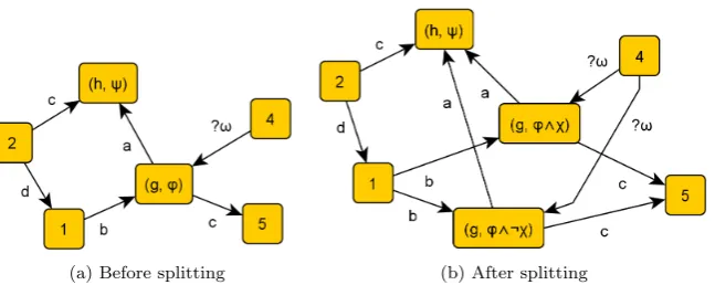
Abstractions can be refined to include new information. When we want to distinguish between states that do or do not satisfy a propertyψ, we can refine the partitions in an abstraction in the following way. See Figure 4.2 on the next page for an example.

Definition 4.14 (Splitting a node). LetA= (N, E) be an abstract program, S= (g, ϕ) a node inAandψa formula that will be used to splitS. We define the abstractionA0 = (N0, E0) that is the result of splittingS byψas follows.

DefineS− = (g, ϕ∧ ¬ψ) and S+_{= (g, ϕ∧ψ). The nodes ofA}0 _{are defined}

by

N0=N∪

(a) Before splitting (b) After splitting

Figure 4.2: Splitting the node (g, ϕ) usingχ

We do not want to change anything essential about the edges. IfS is part of an edge inE, then we want two edges inE0_{, one whereS}−_{has the same role}

as S and one with S+ _{in the same role. By definition an abstraction does not}

contain an edge from a node to itself, so the edge (S, a, S) does not exist in E. Using this, we can define the edgesE0 by

E0 = E∩(N0× A ×N0)

∪

S−, a, T|(S, a, T)∈E

∪

S+, a, T|(S, a, T)∈E

∪

T, a, S−|(T, a, S)∈E

∪

T, a, S+

|(T, a, S)∈E .

Note that splitting a node does not introduce edges of the form (T, a, T). Hence,A0 is an abstraction.

Lemma 4.15. Let A and A0 be abstractions where A0 is obtained from A by splitting a node. IfAis an overapproximation, thenA0 is an overapproximation.

Proof. LetS= (g, ϕ) be the node that has been split using a formulaψ. Letγ be a path with satisfying traceσ

γ = h0

a1

→. . .an

→hn σ = (s0, . . . , sn).

SinceA is an overapproximation, there exists formulaχi such thatsi χi and the path Γ given below is a path in the abstraction.

Γ =S0

a1

→. . . an

→Sn withSi= (hi, χi).

We will replace each nodeSin Γ to obtain a path Γ0 inA0. The edge-labels of Γ0 will be the same as in Γ, we construct the nodesS0_i as follows. If Si6=S then S_i0 =Si. Else if Si =S and si ψ then we take S0i =S+ = (g, ϕ∧ψ). Otherwise,S_i0=S−= (g, ϕ∧ ¬ψ).

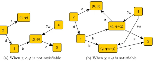
(a) Whenχ∧ϕis not satisfiable (b) Whenχ∧ϕis satisfiable

Figure 4.3: Splitting the transition from (g, ϕ) to (h, ψ) with edge-labela

When the algorithm has encountered a false counterexample, we want to incorporate this information in the abstraction. A false counterexample is a path in the abstraction from (I, ϕpre) to (F,¬ϕpost) that cannot be satisfied by a concrete trace. Hence, we want to delete this path in the abstraction. Since the transitions of this path can be used by other paths that we do not want to delete, we will use the weakest precondition of an action to split the nodes along this path and delete the edges for which we are sure that no path can take them.

First we define how to split along one transition, then we will define how to split along a full path using the first definition. For both we will prove that an overapproximation will stay an overapproximation.

Definition 4.16 (Splitting along a transition). LetS = (g, ϕ) andT = (h, ψ) be two nodes in the abstract programAwith an edge fromS toT labeled with a∈ A. See Figure 4.2a on the preceding page for an illustration. We obtain a new abstract program by splitting this transition as follows.

Letχbe WPa(ψ). We check whetherχ∧ϕis satisfiable. If it is not, let the resulting abstraction be the same as Aexcept that the edge from S to T with labelais removed. The resulting abstraction is given in Figure 4.3a.

Else, letA0 be the abstract program where (g, ϕ) is split usingχaccording to the previous definition. LetS−= (g, ϕ∧ ¬χ) andS+_{= (g, ϕ∧χ) be the new}

nodes. Then let the resulting abstraction be A0 where the edge from S− to T is removed. See Figure 4.3b for an illustration of the resulting abstraction.

Lemma 4.17. Let A and A0 be abstractions where A0 is obtained from A by splitting along a transition. If A is an overapproximation, thenA0 is an over-approximation.

Proof. Let the transition from (g, ϕ) to (h, ψ) with edge-labelabe the transition that has been split. Defineχ= WPa(ψ).

Supposeχ∧ϕis satisfiable. Then the node (g, ϕ) is first split usingχ. This results in an abstractionB that is an overapproximation by Lemma 4.15.

Letγ be a path in the control flow graph that is satisfied by a traceσ

γ = g0

a1

→. . .an

Since B is an overapproximation, there are formulas ψi such that si ψi and Γ defined below is path in the abstraction B.

Γ =S0

a1

→. . .an

→Sn withSi= (gi, ψi).

To see that Γ is also a path inA0, assume otherwise. Hence, there exists an iwithSi = (g, ϕ∧ ¬χ),Si+1= (h, ψ) andai+1=a. Since (si, si+1)∈ R(a) and

si+1 ψ, we have siWPa(ψ) =χby the definition of weakest precondition. This contradicts withsi¬χ. We conclude thatA0 is an overapproximation.

Otherwise,χ∧ϕis not satisfiable. The proof is similar to the second part of the previous case, namely takeB =A.

Definition 4.18 (Splitting along a path). Let S0, . . . , Sn be a path in the abstract program A with edge-labels a1, . . . , an. First we split A along the transition Sn−1, Sn with label an. If this split resulted in new states S+ and S−, and we haven >1, then we recursively split along the pathS0, . . . , Sn−1, S+

with edge labelsa1, . . . , an−1. Else we are finished.

Lemma 4.19. Let A and A0 be abstractions where A0 is obtained from A by splitting along a path. If Ais an overapproximation, then A0 _{is an}

overapprox-imation.

Proof. Splitting along a path is defined by repeatedly splitting along a transi-tion. The result follows from repeatedly applying Lemma 4.17.

The abstraction refinement algorithm will search for a path from (I, ϕpre) to (F,¬ϕpost) in each iteration. The following arguments show that these nodes will always be present in the abstraction.

Fact 4.20. By definition the last node Sn is not split when splitting along the path S0, . . . , Sn.

Lemma 4.21. Let Γ be a path with nodes S0, . . . , Sn whose path constraint is unsatisfiable. Splitting along this path does not split the first nodeS0.

Proof. LetSi= (gi, ϕi) and leta1, . . . , anbe the edge-labels of the path Γ. We prove the contraposition of the Lemma.

Assume S0 has been split. Then all nodes Si with i < n are also split, let S_i− andS_i+ = (gi, ϕ+i ) be the resulting states. Define ϕ+n =ϕn. We will prove with (downward) induction to i that ϕ+_i is the path constraint ρi of the path Si, . . . , Sn.

Leti=n. The path constraintρnof the pathSnisϕn which is by definition ϕ+

n.

Let i < n. The formula used to split Si is WPai+1(ϕ

+

i+1), so ϕ +

i = ϕi∧ WPai(ϕ

+

i+1). The path constraintρi is defined as ρi=ϕi∧WPai+1(ρi+1). By the induction hypothesis, ρi+1 = ϕ+i+1. Hence, ϕ

+

i = ρi. This concludes the induction proof.

Since splitting the transition from S0 to S1+ resulted in S0 being split, we

have by Definition 4.16 that ϕ0∧WPa1(ϕ

+ 1) = ϕ

+

0 is satisfiable. Hence, the

path constraintρ0 of the pathS0, . . . , Sn is satisfiable.

Proof. The nodes (I, ϕpre) and (F,¬ϕpost) are introduced in the abstraction at step 2. The only place where the abstraction changes after step 2 is in step 3(e). The node (F,¬ϕpost) has no outgoing edges, so it can only occur as the last node in a path. By Fact 4.20 we have that (F,¬ϕpost) will always be present in the abstraction.

The node (I, ϕpre) has no incoming edges, so it can only occur as the first node in a path. In the algorithm paths are only split when their path constraint is unsatisfiable, the result follows from Lemma 4.21.

4.6

Correctness

We will first prove that when α does not satisfy its specification, there will always exist a (true or false) counterexample in overapproximations ofα. Then we prove that if a counterexample has a satisfiable path constraint,αdoes not satisfy its specification. Observing that the abstractions used in the abstraction refinement algorithm are always overapproximations, we are then able to prove the correctness of the algorithm itself.

Lemma 4.23. If M 2 ϕpre→ [α]ϕpost andA is an overapproximation of α, then there exists a path Γ inA that starts at(I, ϕpre)and ends at(F,¬ϕpost).

Proof. There exists a s ∈ Σ with s ϕpre∧ hαi¬ϕpost. By the structural operational semantics there is a trace (r0, . . . , rn) withs=r0 andrn¬ϕpost that satisfies a pathγfromItoF in the control flow graph ofα. Letg0, . . . , gn be the nodes ofγ.

Since A is an overapproximation there exists a path Γ with nodes (gi, ψi) such that ri ψi. There are only two nodes in A of the form (I, ψ), namely (I, ϕpre) and (I,¬ϕpre). Sinceg0=I,r0ϕprewe have ψ0=ϕpre.

Similarly, there are only two nodes of the form (F, ψ), namely (F, ϕpost) and (F,¬ϕpost). Since gn =F, rn ¬ϕpost we have ψn =¬ϕpost. Hence, Γ starts at (I, ϕpre) and ends at (F,¬ϕpost).

Lemma 4.24. If the path constraint ρof a path Γ that starts at (I, ϕpre)and ends at (F,¬ϕpost)is satisfiable, then M 2ϕpre→[α]ϕpost.

Proof. Let (g0, ϕ0), . . . ,(gn, ϕn) be the nodes of Γ anda1, . . . , anits edge-labels. Since the path constraint is satisfiable, there exists a s ∈ Σ with s ρ. By Lemma 4.13 there is a trace s0, . . . , sn that satisfies the path with nodes g0, . . . , gn and edge-labels a1, . . . , an and s0 ϕpre and sn ¬ϕpost. By the definition of structural operational semantics we have (s0, sn)∈ Isos(α). Hence,

s0ϕpre∧ hαi¬ϕpost soM 2ϕpre→[α]ϕpost.

Lemma 4.25. The abstract programA is an overapproximation at every stage of the algorithm.

Proof. WhenA is initialized, it is an overapproximation by Lemma 4.11. The abstraction Ais changed in step (2) in the algorithm, see Listing 4.1. It stays an overapproximation by Lemma 4.15.

Theorem 4.26. If the algorithm terminates, its output is correct.

Proof. The algorithm can terminate at two places. Suppose the algorithm termi-nates at step (3b) outputting thatαis correct. This means that there is no path Γ in abstractionAof that stage that starts at (I, ϕpre) and ends at (F,¬ϕpost). By Lemma 4.25 we have that the abstractionAof that stage is an overapprox-imation. By the contraposition of Lemma 4.23 we haveM ϕpre →[α]ϕpost, so αis indeed correct.

Chapter 5

Deterministic propositional

dynamic logic

Propositional dynamic logic allows for non-determinism in two ways. The code constructsα1∪α2andα∗are non-deterministic and actions can result in different

states. An example of the last category is the action p:=random defined in the NDB language in Section 2.3.

Most imperative languages only have deterministic code constructs and most statements execute deterministically. This can be used to make the abstraction refinement algorithm more efficient and it will also enable us to give the fol-lowing termination result. When a deterministic program does not satisfy its specification, the abstraction refinement algorithm will eventually terminate and output that the program is incorrect.

Although non-deterministic actions do not usually occur in programming languages, they are still useful to model the environment of a program. We shall therefore allow arbitrary mixes between deterministic and non-deterministic ac-tions and we will adapt the abstraction refinement algorithm to exploit deter-minism when present. Note that the termination result only holds when all actions are deterministic.

In Section 5.1 we define the language and semantics of a fragment of propo-sitional dynamic logic that only contains deterministic code constructs. Then in Section 5.2 we formally define the two ways in which a program can be deter-ministic and we prove that the fragment of PDL we have defined satisfies this definition.

Then in Section 5.3 we adapt the abstraction refinement algorithm to make use of determinism when present. This allows us to prove the termination result in Section 5.4.

Finally, we run this version of abstraction refinement on the program we presented in the introduction. The results of this verification are discussed in Section 5.5.

5.1

Language and semantics

Definition 5.1. Let (P,A) be a signature. Define the deterministic PDL for-mulas Φd and programs Πd by simultaneous recursion. Let p ∈ P, b ∈ B,

ϕ1, ϕ2∈Φdandδ1, δ2∈Πd, then

ϕ ::= > |p| ¬ϕ1|ϕ1∧ϕ2| hδ1iϕ1

δ ::= b|δ1;δ2|if(ϕ){δ1}else{δ2} |while(ϕ){δ1}.

We use the same models for D-PDL as we use for PDL, see Definition 2.4 on page 6. We give the denotational semantics by defining a translationπfrom D-PDL to PDL. We define π by recursion, the only interesting cases are the new constructs, for completeness we also give the other cases.

π(>) = >

π(p) = p

π(¬ϕ) = ¬π(ϕ)

π(ϕ1∧ϕ2) = π(ϕ1)∧π(ϕ2)

π(hδiϕ) = hπ(δ)iπ(ϕ).

π(b) = b

π(δ1;δ2) = π(δ1);π(δ2)

π(if(ϕ){δ1}else{δ2}) = (?ϕ;π(δ1))∪(?¬ϕ;π(δ2))

π(while(ϕ){δ1}) = (?ϕ;π(δ1))

∗

; ?¬ϕ.

Recall thatIds is the notation for the denotational semantics of PDL

pro-grams and Isos for the structural operational semantics. For D-DPL programs

we use the notation Id dsandId sosfor the two semantics.

Definition 5.2 (Denotational semantics). The denotational semantics ofδ ∈

Πd is defined byId dsM (δ) =I

M

ds(π(δ)).

We could define the control flow graph of deterministic programs using the translation to PDL. However, in the case of the while statement it would not be clear from the control flow graph that this statement is deterministic. We therefore define the control flow graph of deterministic programs separately. Recall thatG(α) is the notation for the control flow graph of a PDL program, we will useGd(δ) for the control flow graph of a D-PDL program.

Definition 5.3. Letδ ∈Πd be a program. We define its control flow graph

Gd(δ) with induction to the structure ofδ. See Figure 5.1 on the next page for

an illustration.

Case1. δ=b. Define Gd(b) as the graph with two nodesI and F, with an

edge fromI toF labeled with the actionb.

Case2. Recursive cases. Let G1 = Gd(δ1) and G2 = Gd(δ2) be the

con-trol flow graphs ofδ1 and δ2 and let I1, I2 andF1, F2 denote their

respective initial and final nodes.

Case i. δ=δ1;δ2. First defineG as the disjoint union ofG1 and

G2. Set I=I1 and F =F2 and merge the node F1 with

(a) The control flow graph ofb

(b) The control flow graph ofδ1 (c) The control flow graph ofδ2

(d) The control flow graph ofδ1;δ2

(e) The control flow graph ofif(ϕ){δ1}else{δ2}

(f) The control flow graph ofwhile(ϕ){δ1}

Case ii. δ=if (ϕ){δ1}else{δ2}. Define G as the disjoint union

ofG1, G2 and a new nodeI. SetF =F1 and merge the

nodesF1 withF2. Add an edge from Ito I1 labeled with

?ϕand add an edge fromI toI2labeled with ?¬ϕ.

Case iii. δ=while(ϕ){δ1}. Define Gas the disjoint union ofG1

with two new nodesI andF. Add the edgesI →I1 and

F1 → I1 both with label ?ϕ, and add the edges I → F

andF1→F both with label ?¬ϕ.

Like PDL programs, we define the structural operational semantics using control flow graphs.

Definition 5.4 (Structural operational semantics). Let M be a PDL-model. Define the GFC-model K in the same way as in Definition 3.10 on page 15. Then define

IM

d sos(δ) =I

K

graph(Gd(δ)).

Proposition 5.5. LetM be a PDL-model. The structural operational interpre-tation IM

d sos(δ)equals the denotational interpretationId dsM (δ).

Proof. LetK be the GFC-model as defined in Definition 3.10 on page 15. The following equalities hold

IM

d ds(δ) = I

M

ds(π(δ)) by definition ofId ds

= IM

sos(π(δ)) by Theorem 3.15

= IK

graph(G(π(δ))) by definition ofIsos

IM

d sos(δ) = IgraphK (Gd(δ)).by definition ofId sos.

We will prove with induction to the structure of δ that a trace (s0, . . . , sn) satisfies a path inG(π(δ)) if and only if it satisfies a path inGd(δ). The

while-statement is the only case whereGd(δ) has a different structure thanG(π(δ)),

this will be the most interesting case.

Case1. δ=b. We haveπ(b) =bandG(b) =Gd(b).

Case2. δ = δ1;δ2. We have π(δ) = π(δ1);π(δ2). The graph G(π(δ)) is in

the same way constructed from G(π(δ1)) and G(π(δ2)) as Gd(δ) is

constructed from Gd(δ1) and Gd(δ2). The result follows from the

induction hypothesis.

Case3. δ=if (ϕ){δ1}else{δ2}. We have

G(π(δ)) =G((?ϕ;π(δ1))∪(?¬ϕ;π(δ2))).

This graph is in the same way constructed fromG(π(δ1)) andG(π(δ2))

as Gd(δ) is constructed fromGd(δ1) and Gd(δ2). The result follows

from the induction hypothesis.

Case4. δ=while(ϕ){δ1}. We have

G(π(δ)) =G (?ϕ;π(δ1))

∗

; ?¬ϕ

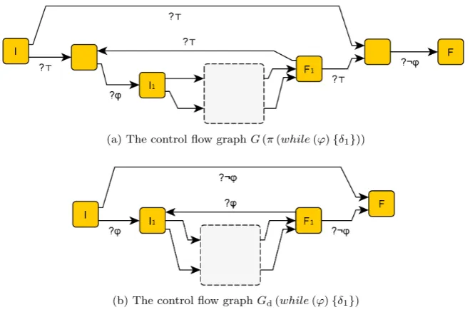
(a) The control flow graphG(π(while(ϕ){δ1}))

(b) The control flow graphGd(while(ϕ){δ1})

Figure 5.2: Equivalent control flow graphs

See Figure 5.2 for an illustration. From the figure it follows that every path inGd(δ) corresponds with a path inG(π(δ)) by inserting edges

?>, and every path inG(π(δ)) corresponds with a path inGd(δ) by

removing edges ?>. SinceR(?>) ={(s, s)|s∈Σ}, a satisfying trace of a path in Gd(δ) corresponds with a satisfying trace of the

corre-sponding path inG(π(δ)) by the induction hypothesis and doubling statessin the trace when an edge ?>is inserted. And in the other direction, a satisfying trace of a path in G(π(δ)) corresponds with a satisfying trace of the corresponding path inGd(δ) by the induction

hypothesis and merging two adjacent statess, sin the trace tosfor every removed edge ?>.

5.2

Determinism

There can be two different types of determinism in a program. One is that at every stage there is only one statement that can be executed next, the other is that a single statement can only result in one state.

We define this in the languages of control flow graphs, let A be a CFG-signature andK= (Σ,R) a CFG-model.

Definition 5.7(Deterministic relation). A relationR⊆Σ×Σ is deterministic if it is a partial function. That is, for every s∈ Σ there is at most one r∈Σ with (s, r)∈R.

Definition 5.8 (Deterministic action). An actiona∈ Ais deterministic inK if the relationR(a) is deterministic.

We will prove that the control flow graphs of D-DPL programs are deter-ministic control flow graphs. First observe the following from the definition of Gd.

Fact 5.9. LetGbe the control flow graph of a programδ, then the node labeled F has no outgoing edges.

Lemma 5.10. The graphGd(δ)is a deterministic control flow graph.

Proof. We prove this with structural induction onδ. Lets∈Σ be a state,g a node inGd(δ) ande1, . . . , en be the outgoing edges ofg.

Case1. δ=b. ThenGd(δ) has only one edge.

Case2. δ = δ1;δ2. If g 6= F2]I2, then g and its outgoing edges are fully

contained in eitherGd(δ1) orGd(δ2). Ifg=F2]I2, we have by Fact

5.9 that the outgoing edges of g are contained in Gd(δ2). In both

cases the result follows from the induction hypothesis.

Case3. δ = if (ϕ){δ1}else{δ2}. When g = F, it has no outgoing edges.

When g = I the outgoing edges are ?ϕ and ?¬ϕ. If s ϕ there cannot be a r with (s, r) ∈ R(¬ϕ) and when s 2 ϕ there cannot

be ar with (s, r)∈ R(?ϕ). Hence, there is at most one i with the asked property. Ifg6=F andg6=I, we have thatg and its outgoing edges are fully contained in eitherGd(δ1) orGd(δ2). Then the result

follows from the induction hypothesis.

Case4. δ =while(ϕ){δ1}. Wheng =F, it has no outgoing edges. When

g=I org=F1 the outgoing edges are ?ϕand ?¬ϕ. The argument

is the same as in the previous case. Otherwise, we have thatg and its outgoing edges are fully contained inGd(δ1) and the result follows

from the induction hypothesis.

To connect D-DPL with the second type of determinism, we prove that if all actions are deterministic the interpretation of a D-DPL program is deterministic.

Lemma 5.11. Suppose all actions b∈ B are deterministic in M. Let γ1 and

γ2 be two paths inGd(δ) of length n that start at a node g. Let s∈Σ, let σ1

and σ2 be two traces starting with s that satisfy respectively γ1 and γ2. Then

σ1=σ2 andγ1=γ2.

Proof. We prove this with induction to n. If n = 1 then σ1 = σ2 since they

both start withs.

Letn >1. Letg1 be the second node of γ1, r1 the second state of σ1 and

(s, r1)∈ R(a1) and (s, r2)∈ R(a2) andGdis a deterministic control flow graph

by Lemma 5.10, we have that g1 =g2 and a1 =a2. If a1 is a test action, we

have s =r1 =r2. Else,a1 is a basic action and by assumption deterministic.

Hence,r1=r2. The result follows from the induction hypothesis.

Proposition 5.12. Suppose all actionsb∈ Bare deterministic in M. Letδbe a program, then its interpretationIM_{(δ)is a deterministic relation.}

Proof. Suppose (s, r1)∈ IM(δ), (s, r2)∈ IM(δ). By the structural operational

semantics, there are pathsγ1,γ2in the graphGd(δ) that are satisfied by traces

σ1andσ2, where both traces start withs,σ1ends withr1 andσ2ends withr2.

Letn1, n2 be their lengths. Suppose n1 ≤n2. Look at the first n1 nodes

of γ2. By Lemma 5.11 we have that this segment equals γ1. Hence, the n1-th

node of γ2 is F. By Fact 5.9 F has no outgoing edges and we conclude that

n1 =n2. When n1≥n2 the argument is the same, hence n1 =n2. We apply

Lemma 5.11 again to see thatr1=r2.

5.3

Partition refinement on D-PDL

The partition refinement algorithm defined in Chapter 2 is defined over PDL programsα∈Π. However, it only uses the control flow graphG(α) to verifyα and not the specific PDL constructs. When we replaceG(α) byGd(δ), we can

therefore use the same definitions and proofs to define the algorithm on D-PDL. The second change we make in the algorithm is that we use a different way of splitting along a path. This definition makes the algorithm more efficient when it splits along a path that contains deterministic actions.

The last change is that the algorithm searches for the shortest abstract path from (I, ϕpre) to (F,¬ϕpost) instead of an arbitrary path. This enables us to give a proof that the algorithm terminates on incorrect programs.

The algorithm is given in Listing 5.1 on the next page together with refer-ences to the relevant definitions and proofs.

Refinements

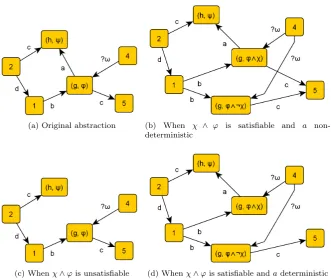
When we know that an action is deterministic, we can remove more edges when we split along a transition labeled by that action. See Figure 5.3 on page 40 for an illustration of all the possible cases.

Definition 5.13 (Splitting along a transition). LetS = (g, ϕ) andT = (h, ψ) be two nodes in the abstract programAwith an edge fromS toT labeled with a∈ A. We obtain a new abstract program by splitting this transition as follows. First we refine the abstraction according to Definition 4.16 on page 28. Re-call that when χ∧ϕ is not satisfiable where χ = WPa(ψ), this results in an abstraction as shown in Figure 5.3c. When it is satisfiable it results in an abstraction as shown in Figure 5.3b.

When this refinement causedSto be split intoS− _andS+_{andais a}

deter-ministic action, we additionally do the following. We remove all outgoing edges fromS+_{except the edge toT labeled witha. An illustration is shown in Figure}

Listing 5.1 The abstraction refinement algorithm on D-PDL

The algorithm

1. Initialize the abstraction A as the deterministic control flow graph of δ where each node is associated with the formula>.

2. Split (I,>) into (I, ϕpre) and (I,¬ϕpre). Split (F,>) into (F, ϕpost) and (F,¬ϕpost).

3. Repeat the following

(a) Find the shortest abstract path S0, . . . , Sn in A withS0 = (I, ϕpre) andSn= (F,¬ϕpost).

(b) If such a path does not exist, output thatδis correct. Else, continue.

(c) Fori∈ {0, . . . , n}letρi be the path constraintρi ofS0, . . . , Si. Find the smallest isuch thatρi is not satisfiable.

(d) If such an i does not exist, output that δ is incorrect. Continue otherwise.

(e) Change the abstractionAby splitting along the path S0, . . . , Si.

Explanation

1. Abstractions and the initial abstraction are defined analogously to Defini-tion 4.7 and 4.8 on page 24, where we use the deterministic control graph Gd(δ) in stead ofG(α).

2. In Definition 4.14 on page 26 it is defined how to split nodes.

3. In each iteration the abstractionAis changed, or the algorithm terminates.

(a) An abstraction is a finite directed graph.

(b) The correctness is proved in Theorem 5.17.

(c) Path constraints are defined in Definition 4.12 on page 26.

(d) The correctness is proved in Theorem 5.17.

(a) Original abstraction (b) When χ ∧ ϕ is satisfiable and a non-deterministic

(c) Whenχ∧ϕis unsatisfiable (d) Whenχ∧ϕis satisfiable andadeterministic