Non linear unsteady wave loads on large high speed wave piercing catamarans

Full text

(1)c.e du .au. iam. BY. in@. am. NON-LINEAR UNSTEADY WAVE LOADS ON LARGE HIGH-SPEED WAVE PIERCING CATAMARANS.. wa. WALID AMIN BSc (Hons) (1995), MSc Naval Architecture and Marine Engineering, Alexandria. Wa. lid. Am. in,. University (2000). Co. py. Rig. ht. Submitted in fulfilment of the requirements for the degree of Doctor of Philosophy at the UNIVERSITY OF TASMANIA. May 2009. 1.

(2) c.e du .au am. in@. To whom we owe most. iam. To whom we love most. wa. To whom we respect most. in,. To Raham. Am. To Karma, Nourin and Taha. Co. py. Rig. ht. Wa. lid. To my parents. 2.

(3) DECLARATION OF ORIGINALITY This Thesis contains no material that has been accepted for a degree or diploma by the. c.e du .au. University of Tasmania or any other institution, and to the best of my knowledge and belief no material previously published or written by another person except where due. May 2009.. Co. py. Rig. ht. Wa. lid. Am. in,. wa. iam. Walid Amin. in@. am. acknowledgement is made in the text of the thesis. 3.

(4) STATEMENT OF AUTHORITY OF ACCESS This thesis is not to be made available for loan or copying for two years following the date. c.e du .au. this statement was signed. Following that time the thesis may be made available for loan. in@. am. and limited photocopying in accordance with the copyright Act 1968.. Co. py. Rig. ht. Wa. lid. Am. in,. wa. iam. Walid Amin May 2009.. 4.

(5) ABSTRACT The current work investigates the slamming characteristics of wave piercing catamarans. c.e du .au. through the analysis of sea trials data of the 98 m Incat sea frame “Hull 061”, built in Tasmania, Australia and currently serving in the US Navy combat fleet. The importance of this sea trials data is that the ship was tested in severe sea conditions to assess her suitability for military operations and to define her operational envelope. New signal processing techniques such as Wavelet Transforms are used in analysing slamming data for two main. am. purposes, slamming identification and modal analysis in time and frequency domains simultaneously. The Wavelet Transforms were found superior to conventional signal. in@. processing tools such as Fast Fourier Transform and Short Time Fourier Transform. The structural strength of wave piercing catamarans is studied by introducing a novel sea. iam. trials analysis for structural performance assessment in an attempt to simulate real loading conditions. The methodology was tested on normal linear wave loading (without. wa. slamming) and was found satisfactory. A “Reverse Engineering” approach is introduced to predict slamming loads during sea trials by using the capabilities of Finite Element Analysis. in,. using the well known software PATRAN/NASTRAN1. To increase the efficiency of this. Am. approach, the load parameters, spatial location and distribution, were investigated through model tests of a similar but larger 112 m Incat hydro-elastic model in the Australian. lid. Maritime College towing tank facility. Based on pressure measurements, proper slam load. Wa. models can be more accurately and efficiently introduced in the finite element analysis. Quasi-static analysis was first performed to examine its suitability to analyse such fast time. ht. varying loads. Difficulties in comparison procedures between numerical simulations and. Rig. trials data have strongly highlighted the need for dynamic analysis. Direct transient dynamic analysis was performed using the dynamic solver of the same software package. Good agreement with trials data was found. The suggested procedure and slamming loading. py. patterns used in the numerical simulation is then verified and can be regarded as a solid. Co. base for verification of other theoretical design models.. 1. MSC Software Corporation, USA. 5.

(6) ACKNOWLEDGEMENT I would like to express my gratitude to my colleagues at the University of Tasmania,. c.e du .au. Australian Maritime College, Revolution Design and Incat Tasmania for the support they have provided during the course of this project.. Special thanks are due to Professor M. R. Davis from the University of Tasmania for his ongoing support and encouragement. He inspired me with his attitude of hard working. am. and decency during our discussions and his approach to explore the unknown by “learning on the job”.. in@. I am particularly grateful to Dr Giles Thomas from the Australian Maritime College for his ongoing support through the duration of my candidature. It is just simple to say without. iam. his support, encouragement and dedication a big part of this project wouldn’t have seen the light. Special appreciation is owing to Dr Holloway for his fine technical support and. wa. intelligent suggestions.. in,. I want to thank the team work in Revolution design, especially Mr. Gary Davidson for his support even, during his busy schedule; as well as Mr. Tim Roberts for his encouragement. Am. and support.. lid. Finally, there is a real hero behind this work. She was working in silence, providing sincere and ongoing support, encouraging, guiding, motivating and inspiring me for harder work. Wa. and better results. Without her support, I would not finish such a job. Words are not. ht. enough to express my gratitude. Thank you Raham.. Rig. At last, I want to express my gratitude to my parents, brothers and sisters for their. Co. py. continuous encouragement.. 6.

(7) CONTENTS NON-LINEAR UNSTEADY WAVE LOADS ON LARGE HIGH-SPEED WAVE PIERCING CATAMARANS. ............................................................................................................................................ 1. c.e du .au. DECLARATION OF ORIGINALITY ....................................................................................................... 3 STATEMENT OF AUTHORITY OF ACCESS ....................................................................................... 4 ABSTRACT .................................................................................................................................................... 5 ACKNOWLEDGEMENT ............................................................................................................................ 6 CONTENTS .................................................................................................................................................. 7 INTRODUCTION ............................................................................................................................ 10 BACKGROUND ................................................................................................................................. 10 STRUCTURAL CONFIGURATION OF INCAT WAVE PIERCING CATAMARANS....................................... 15 PROBLEM DEFINITION ..................................................................................................................... 16 SCOPE OF WORK............................................................................................................................... 20 GENERAL ARRANGEMENT OF THE THESIS....................................................................................... 23. am. 1.1 1.2 1.3 1.4 1.5. in@. 1. iam. 2 SLAMMING CHARACTERISTICS OF HULL 061, HSV-2 SWIFT, USING WAVELET TRANSFORMS............................................................................................................................................ 25 INTRODUCTION AND SCOPE OF WORK ............................................................................................ 25 SEA TRIALS ....................................................................................................................................... 26 2.2.1 Data analysis ............................................................................................................................ 27 2.2.2 Strain gauges selection.................................................................................................................. 27 2.2.3 Processing of strain gauges data ..................................................................................................... 29 2.2.4 Processing of seakeeping data ........................................................................................................ 30 2.3 SLAMMING INVESTIGATION VIA TIME AND/OR FREQUENCY DOMAINS .......................................... 31 2.3.1 Time series representation in time-frequency space .............................................................................. 38 2.3.2 Continuous wavelet transform ....................................................................................................... 39 2.3.3 Slamming signature in wavelet transform......................................................................................... 50 2.3.4 Modal parameters identification..................................................................................................... 55 2.3.5 Application of wavelet transform to sea trials signals ......................................................................... 62 2.4 SLAMMING CHARACTERISTICS OF HSV-2 SWIFT ............................................................................ 86 2.4.1 Slamming identification procedure .................................................................................................. 86 2.4.2 Maximum slamming responses ..................................................................................................... 90 2.4.3 Peak-trough analysis ................................................................................................................... 92 2.4.4 Slam location ............................................................................................................................. 96 2.4.5 Pitch effect ............................................................................................................................... 104 2.4.6 Effect of bow vertical relative velocity ............................................................................................. 104 2.5 CONCLUSIONS ................................................................................................................................ 112. Rig. ht. Wa. lid. Am. in,. wa. 2.1 2.2. 3 EXPERIMENTAL PRESSURE MEASUREMENTS ON THE CENTRE BOW AND THE WETDECK. ................................................................................................................................................ 115. py. INTRODUCTION ............................................................................................................................. 115 MOTIVATION AND SCOPE OF WORK .............................................................................................. 122 EXPERIMENT SETUP ....................................................................................................................... 124 3.3.1 Testing facility description ........................................................................................................... 124 3.3.2 Model description...................................................................................................................... 125 3.4 INSTRUMENTATION ....................................................................................................................... 128 3.4.1 Pressure transducers .................................................................................................................. 128 3.4.2 Wave probes ............................................................................................................................ 130 3.4.3 LVDT .................................................................................................................................. 130 3.4.4 DAQ system description and properties ........................................................................................ 130 3.5 TEST PLAN AND PROCEDURE ......................................................................................................... 132 3.5.1 Phase (A) set up ...................................................................................................................... 133. Co. 3.1 3.2 3.3. 7.

(8) 4. c.e du .au. 3.5.2 Phase (B) set up ....................................................................................................................... 134 3.5.3 Phase (C) set up ....................................................................................................................... 134 3.5.4 Phase (D) set up ...................................................................................................................... 137 3.6 RESULTS ANALYSES ........................................................................................................................ 137 3.6.1 The appropriate sampling rate ..................................................................................................... 137 3.6.2 The effect of hydro-elasticity ......................................................................................................... 140 3.6.3 Longitudinal pressure distribution................................................................................................ 145 3.6.4 Pressure mapping...................................................................................................................... 168 3.7 CONCLUSIONS ................................................................................................................................ 182 QUASI-STATIC ANALYSIS OF NON-LINEAR WAVE LOADS. .......................................... 184 INTRODUCTION ............................................................................................................................. 184 PROBLEM DEFINITION AND SCOPE OF WORK ................................................................................ 186 SELECTION OF TRIALS DATA SAMPLE FOR METHODOLOGY VALIDATION ..................................... 188 FINITE ELEMENT MODEL DEVELOPMENT ..................................................................................... 193 4.4.1 Modelling techniques ................................................................................................................. 194 4.4.2 Model adjustments and mesh refinement........................................................................................ 198 4.4.3 Wave load model ...................................................................................................................... 204 4.5 RESULTS AND DISCUSSION ............................................................................................................. 216 4.6 QUASI STATIC ANALYSIS OF SLAM LOADS ....................................................................................... 228 4.6.1 Simulation of slamming loads ..................................................................................................... 228 4.6.2 The instant of Slam occurrence .................................................................................................... 229 4.6.3 Slam load spatial distribution ..................................................................................................... 230 4.6.4 Slam load case development ........................................................................................................ 234 4.6.5 Comparison with trials .............................................................................................................. 236 4.6.6 The quasi-static impulse............................................................................................................. 240 4.7 CONCLUSIONS ................................................................................................................................ 247. wa. iam. in@. am. 4.1 4.2 4.3 4.4. STRUCTURAL DYNAMIC ANALYSIS OF NON-LINEAR WAVE LOADS....................... 250. in,. 5. INTRODUCTION ............................................................................................................................. 250 REAL EIGENVALUE ANALYSIS ........................................................................................................ 250 5.2.1 Dry modal analysis ................................................................................................................... 252 5.2.2 Wet modal analysis................................................................................................................... 257 5.3 DIRECT TRANSIENT RESPONSE ANALYSIS ...................................................................................... 261 5.3.1 Difficulties associated with full dynamic analysis ............................................................................. 263 5.3.2 Dynamic loading model ............................................................................................................. 264 5.3.3 Damping ................................................................................................................................ 267 5.4 RESULTS ......................................................................................................................................... 271 5.5 CONCLUSIONS ................................................................................................................................ 274. Wa. lid. Am. 5.1 5.2. 6.1 6.2 7. ht. CONCLUSIONS ............................................................................................................................. 277 OUTCOMES OF THE PRESENT INVESTIGATION .............................................................................. 277 RECOMMENDATIONS FOR FUTURE WORK...................................................................................... 280. Rig. 6. REFERENCES ................................................................................................................................ 283. py. APPENDIX A: HULL 061 SPECIFICATIONS .................................................................................... 296 APPENDIX B: TRIALS CONDITIONS ............................................................................................... 297. Co. APPENDIX C: STRAIN GAUGE LOCATIONS.................................................................................. 298 APPENDIX D: INCAT 112 SPECIFICATIONS ................................................................................... 301 APPENDIX E: PRESSURE TRANSDUCER FACT SHEET ............................................................ 302 APPENDIX F: SIGNAL CONDITIONER FACT SHEET ................................................................ 304 APPENDIX G: PRESSURE SENSING POINT ORDINATES......................................................... 306 APPENDIX H: PHASE C CONDITIONS. .......................................................................................... 309. 8.

(9) APPENDIX I: ALL PHASES TRANSDUCERS LAYOUT TABLE. LOCATION IS ACCORDING TO TAPPING NUMBER IN APPENDIX G. ...................................................................................... 310 APPENDIX J: ACOUSTIC WAVE PROBE SPECIFICATIONS ...................................................... 311 APPENDIX K: SELECTED LOCATIONS FOR PRESSURE MAPPING ...................................... 312. c.e du .au. APPENDIX L: DRY MODAL PARTICIPATION FACTORS ........................................................... 313. Co. py. Rig. ht. Wa. lid. Am. in,. wa. iam. in@. am. APPENDIX M: DRY MODAL EFFECTIVE MASS FRACTION ..................................................... 314. 9.

(10) 1 INTRODUCTION 1.1. Background. c.e du .au. Increased demand in high-speed sea transportation has led to rapid and ongoing development of high-speed marine vehicles especially multi-hull ships. However, the development of multi-hull ships goes back thousands of years ago when it was first presented by the Polynesian seafarers in the form of “proa”, Figure 1.1 and the “precolumbian” raft built by the ancient South Americans, International Polynesian Portal [1].. am. The 17th century witnessed the first modern building of catamarans when the first conceptual catamaran “double-bottom” was built by Sir William Petty in 1660, Pumfrey. Rig. ht. Wa. lid. Am. in,. wa. iam. in@. [2].. Figure 1.1: Artistic presentation of “Proa” boats built by the Polynesians, International Polynesian Portal [1].. py. Steam paddle wheel powered catamarans operating as ferry boats and river craft appeared. Co. in the UK and US in early 1800’s, Clark et al. [3].Since 1980’s to early 1990’s, the number of built catamarans increased rapidly operating as passenger ferries in the range of 25 to 40 m with passenger capacities up to 400 passengers. A typical catamaran during this period is shown in Figure 1.2.. 10.

(11) c.e du .au. in,. wa. iam. in@. am. Figure 1.2: Typical 30 m fast passenger catamaran during 1980’s built by Incat Tasmania.. Co. py. Rig. ht. Wa. lid. Am. Figure 1.3: First car/passenger wave piercing catamaran built by Incat Tasmania, 1993.. Figure 1.4: The 125 m HSS 1500 Stena built by Finnyard, 1996.. At this stage, market demands highlighted the need for car/passenger ferries which finally led to the introduction of new designs which are capable of carrying cars and light weight cargo. The first boat to be built to meet these requirements was the Condor 10, LOA 74 m 11.

(12) and built by Incat Tasmania in 1993. In 1996, Finnyard in Finalnd launced the HSS (high speed ship) “Stena Line”, a 125 m car/passenger ferry that was capable of carrying 1520. iam. in@. am. c.e du .au. passenger, 375 cars and operating at speed of 40 knots, Figure 1.4.. py. Rig. ht. Wa. lid. Am. in,. wa. Figure 1.5: The 96 m HMAS Jervis Bay (HSV-X1) wave piercing catamaran built by Incat Tasmania, 1998.. Co. Figure 1.6: The 98m HSV 2 Swift wave piercing catamaran built by Incat Tasmania, 2003.. The advantages of high speed vessels, with a relatively high payload, drew attention to the applicability of high-speed catamarans in military operations as logistics, transport and rescue support ships. In 1999, Incat Tasmania chartered the first military 86 m boat to the Royal Australian Navy to serve as a fast sea link for Australian troops between Darwin and Dili in East Timor, during the operation of the Australian-led INTERFET peacekeeping. 12.

(13) taskforce. The ship was capable of sailing 430 nautical miles (800 km) in approximately 11 hours, at an average speed of approximately 45 knots (83 km/h), far faster than vessels of comparable size and role in the region. During the two years of the ship's charter by the. c.e du .au. Royal Australian Navy, HMAS Jervis Bay made 107 trips between Darwin and East Timor, shipping 20,000 passengers, 430 vehicles and 5,600 tonnes of freight, becoming known as. in,. wa. iam. in@. am. the "Dili Express".. Am. Figure 1.7: The 80 m X-Craft catamaran, designed by Nigel Gee and Associates Ltd, and built by Nichols Bros. boat builders, Washington, USA.. lid. In 1998, the US Navy chartered its first 96 m wave piercing catamaran known as HSV X1,. Wa. Figure 1.5, to test the new technologies and concepts associated with the Chief of Naval Operations's "Seapower 21" plan. The vessel has the ability to ferry up to 325 combat personnel and 400 tons of cargo up to 3000 miles one way at speeds in excess of 40 knots.. ht. Ordered for the US Navy in 2002, the 98 m Spearhead TSV 1X benefited from. Rig. performance and engineering data gathered through the operation of HSV X1. HSV 2 Swift (the vessel under consideration through this thesis), was completed to the US Navy. py. specification and delivered in 2003. The vessel underwent an extensive sea trials program. Co. to assess her operational envelope for military applications. In 2005, the US navy tested a semi-swath catamaran (without the centre bow configuration) through the X-Craft, an experimental platform for an innovative new class of fast, littoral, warfare craft, designed by BMT Nigel Gee and Associates Ltd. The vessel is the largest catamaran ever to be built in the US and one of the fastest large naval craft in the world and is capable of operation at speeds in excess of 50 knots (in calm seas), Figure 1.7.. 13.

(14) c.e du .au am. lid. Am. in,. wa. iam. in@. Figure 1.8: First wave piercing catamaran, “Tassie Devil 2001”, built by Incat Tasmania in 1986.. Wa. Figure 1.9: The 107 m Hawaii Superferry built by Austal Ships (Western Australia), 2007.. When the use of catamarans extended from sheltered waters to more exposed sea going operation, motion problems in rough seas started to arise. Excessive pitching in following. ht. seas caused severe impacts on the bridging structure that connects the demi-hulls. The. Rig. centre bow conceptual design was first introduced by Philip Hercus (Incat Designs Sydney) to reduce the pitching motion in head and following seas and in particular to avoid deck. py. diving when the bow enters the water in following seas. The first wave piercing catamaran. Co. with a centre bow configuration was built by Incat Tasmania in 1986, Figure 1.8. From that time and on, almost all Incat ships were fitted with centre bows. In contrast, Austal Ships, the main competitor of Incat in the international market, kept the conventional catamaran configuration (with flat wet deck). Austal designs of sea going catamarans have a different strategy to avoid bow diving by introducing a “sufficient” air gap (or tunnel height) so that the wet deck remains relatively clear from the water surface in the designated operation. 14.

(15) conditions. Similar vessels of comparable capacities and lengths to Incat designs have been built such as the 107 m Hawaii Superferries, Figure 1.9. 1.2. Structural configuration of Incat wave piercing catamarans. c.e du .au. In order to familiarise the reader with the novel design of these vessels and the notations. in,. wa. iam. in@. am. used through the thesis, the general structural configuration is presented in this section.. Am. Figure 1.10: Cut away port side section of Incat hull girder showing horizontal and vertical cross bracing.. lid. One of the major characteristics of these vessels is the high service speed they can operate. Wa. at. This high speed can be achieved when lighter structures can be built to the required strength to withstand the environmental loads. Therefore, the first design goal is usually to optimise the deadweight to lightship ratio whilst maintaining structural integrity and. ht. reliability. Thus, structural optimisation is an essential task during the preliminary design. Rig. process. In addition to the normal longitudinal framing system onboard monohulls, cross bracing (in the vertical and horizontal directions) is used to provide structural strength to. py. withstand longitudinal and lateral torsional deformations as shown in Figure 1.10.. Co. The superstructure is supported by transverse beams (the superstructure raft, Figure 1.11) which are connected to the main hull girder through rubber mounts to reduce the vibration levels in the passenger lounges. Incat catamarans are characterised by a centre bow between the demi-hulls. The centre bow length ranges between 19 to 30% of the waterline length. Its main purpose is to counteract the bow diving in following seas as well as reducing the vessel pitching motion by offering extra buoyancy as the bow pitches into the. 15.

(16) wave. Consequently, the vessel has two archways between the centre bow and demi-hulls. in,. wa. iam. in@. am. c.e du .au. in the forward part of the vessel. Behind the centre bow, the wet-deck is flat, Figure 1.12. 1.3. Figure 1.12: Characteristic centre bow of Incat catamarans.. Co. py. Rig. ht. Wa. lid. Am. Figure 1.11: Cross section of Incat hull girder.. Problem definition. When the vessel is operating in rough seas, the ship may experience water impact loads due to the excessive relative motion between the vessel and the waves. A shudder or vibration occurs following such impacts known as whipping. Severe slamming loads might result in abrupt changes in vessel motions and high stress levels which may in turn cause structural. 16.

(17) damage. Such damage has a direct influence on short term cost due to the cost of repair and loss of service time; in addition, long term losses might occur due to bad publicity of. wa. iam. in@. am. c.e du .au. stiff ship motions.. py. Rig. ht. Wa. lid. Am. in,. Figure 1.13: Damage of bow structure on HSS 1500 Stena due to severe slamming loads.. Co. Figure 1.14: Side shell buckling as a consequence of severe slamming loads, Hull 50 of Incat Tasmania.. Slamming on multihull ships is different from slamming on monohulls in terms of slam location and severity. Twin hull ships experience unique type of slamming called wet-deck slamming, when the underside of the cross deck structure comes in contact with the wave surface in the presence of sufficient relative motion between the vessel and the water. 17.

(18) surface. Serious damage occurred on the HSS 1500 Stena bow structure due to a severe slamming event in rough seas, Figure 1.13. Deformation of longitudinal stiffeners has been reported on an 86 m Austal vessel due to. c.e du .au. severe slamming loads, Rothe et al. [4]. On wave piercing catamarans, Hull 050 of Incat suffered side shell buckling, Figure 1.14, and tripping of brackets in the centre bow area, Figure 1.15. In general, severe slamming load effects can result in:. (b) Distortion of centre bow T-bar longitudinal stiffeners.. in@. (c) Side shell buckling.. am. (a) Localised dishing of plating between longitudinal stiffeners and side frames.. iam. (d) Distortion of frames and stiffeners aft of the centre bow.. Rig. ht. Wa. lid. Am. in,. wa. (e) Crack propagations due to the effect of whipping in the form of material fatigue.. Co. py. Figure 1.15: Tripping of brackets and vertical stiffeners in the centre bow of Hull 50 of Incat Tasmania due to severe slamming load.. 18.

(19) c.e du .au am in@. iam. Figure 1.16: Severe vertical bow vertical acceleration during Hull 061 sea trials in head seas, sea state 5, 20 knots speed.. Incat Hull 061 (HSV 2 Swift) has shown greatly improved structural integrity,. wa. demonstrated when the vessel underwent extensive sea trials program by the US Navy to define its operational envelope. The vessel was tested significantly beyond the service. in,. criterion she was designed to withstand according to the DNV rules. Consequently high motion acceleration records were reported, Figure 1.16. As will be shown in this thesis, the. Am. calculated loads during the design process were smaller than those imparted on the structure during trials. However, the ship withstood these high loads without any structural. lid. damage. This means that the ship structure may be further optimised to reduce the. Wa. lightship displacement and consequently increase the payload. However, the calculation of slam loads on large catamarans fitted with a centre bow is a. ht. complex task and extreme loads to date have not been established through a proven. Rig. theoretical approach. Unfortunately the kinematics of slamming events is also not well understood on large high-speed catamarans. Classification of slamming events and the. py. factors affecting the slamming occurrences can only be evaluated by full scale measurement and/or model testing. In comparison to the extensive work that has been done for. Co. slamming on monohulls, such as that due to Aertssen [5]and Iaccarino et al. [6], little work has been published on full scale measurement of loads and motions of large high speed catamarans. Roberts et al. [7] extrapolated sea trials stresses of two 81 m and 86 m Incat catamarans at a probability of 10-8 using Weibull and Gumbel extreme value plots. The analysis assumes that extrapolated full scale stresses can be directly compared with the FE model stresses at the same locations in a quasi-static analysis. Steinmann et al. [8] 19.

(20) extrapolated sea trials extreme value stresses at a probability of 10-8 using the Ochi extrapolation procedure which assumes a linear relationship between stresses and wave height which is not true for moderate to heavy seas for large high speed catamarans.. c.e du .au. Individual slamming events were identified during data post processing. The peak slam responses were compared to the quasi-static global response levels as defined by classification societies. The used extreme value analysis, in both cases, was implemented to compensate for the dynamics of slamming. Thomas et al. [9] and Thomas et al. [10] have explored the slam dynamics extensively without extrapolation techniques to investigate the. am. load values during an extreme slamming event that caused buckling of the superstructure shell plates on an 96 m Incat catamaran during her regular service across Cook Strait in. in@. New Zealand. The investigation resulted in improved understanding of slamming dynamics showing that the slamming load during this particular event is in excess of 1000. iam. tonnes. In the current analysis, the author extended the investigation of slamming dynamics through the improvement of slamming identification techniques, quasi-static and. wa. dynamic finite element analysis (FEA) as well as conducting experimental measurements of dynamic pressures in regular waves on the centre bow and the bridging structure. The key. in,. novel objectives in the current work are:. calibration factors technique.. Am. (a) Introduction of new trials interpretation technique instead of the conventional. lid. (b) The introduction of wavelet transform as a new signal analysis to investigate the ship. Wa. structural performance during sea trials. (c) Hydrodynamic pressure measurements on the centre bow and wet deck structure in. Rig. ht. regular waves.. (d) Introduction of the “reverse engineering” technique in prediction of the linear and non-. Scope of work. Co. 1.4. py. linear wave loads using the capabilities of finite element analysis and sea trials data.. Sea trials analysis is an important approach for assessing new designs and has a direct impact on the evaluation of design methods and numerical models in respect to resistance, seakeeping, structural optimisation and loading models. Sea trials enable the designer to assess the design loading models and formulae used in the original design. Moreover, they help to understand the environmental loads that a ship would sustain in all working. 20.

(21) conditions and how the structure responds to these loads. The sea trials considered in this thesis are for Hull 61, an INCAT seaframe (HSV 2 Swift), originally a fast passenger/ferry design, re-configured for US Navy military purposes. The ship has undertaken extensive. c.e du .au. sea trials to investigate this hull configuration for military purposes and to determine her operational envelope.. A primary motivation behind the current work was the large motion responses observed during trials in high sea states, which exceeded the design values. Excessive accelerations are due to slamming impact loads which are not fully understood for this type of vessel.. am. The goal of this work is to effectively understand the water impact problem, and the. in@. consequential structural loads using the sea trials data combined with the capabilities of finite element analysis. The strategy for achieving the specified goal can be summarised as. iam. follows:. (a) Identification of a signal analysis tool that is suitable for the analysis of non-stationary. wa. signals with transient events. This is required to derive a slamming identification technique. (b) Analysis of slamming kinematics in terms of ship and water surface motion during the. Am. in,. slamming events.. (c) Using finite element analysis capabilities, a quasi-static reverse engineering procedure was established in which a finite element model is loaded arbitrarily (but with input from. lid. the sea trials such as the wave condition, ship motions, etc.). The finite element strains. Wa. were compared to the trials data for specific slam events. The load model was modified until a satisfactory agreement between trials strains and computed strains is achieved.. Rig. ht. (d) A similar comparison approach was repeated using a full FE dynamic analysis. The reverse engineering procedure is usually conducted when available theoretical models. py. fail to predict comparable results with experiments or are inadequate for the problem under consideration. There are many methods to calculate the global loads on catamarans. Co. (see Holloway [11], Faltinsen et al. [12], Kring et al. [13], Kring et al. [14], Weems et al. [15], Ito et al. [16], Chan [17] and Chan [18]). However, fewer methods are available for slamming loads. Kvålsvold et al. [19] and Økland et al. [20] concluded that structural elasticity is necessary in the simulation and the predicted slamming loads are conservative when a two-dimensional approach is used. Haugen et al. [21] proposed a three dimensional approach and results were compared to sea trials of a 30 m catamaran satisfactorily. 21.

(22) However, the vessel relative velocity was predicted instead of being extracted from sea trials data. To date these methods have been verified against small size catamarans and without a centre bow configuration and therefore these methods are not suitable for. c.e du .au. analysis of the current vessel. The current methodology of sea trials analysis such as Sikora et al. [22], is based on extraction of calibration factors for the strain gauges by applying a known load (known bending moment value for example) to the finite element model. The calibration factors are load independent and can be regarded as a local property of the position of the strain. am. gauge. Thus, the calibration factors can be regarded as a transfer function between the. in@. applied load and local response. Consequently, if the structural response is known (from trials), then an equivalent loading (similar to the load used in determining the calibration factor but scaled up or down) can be obtained. The method works well for the underlying. iam. wave loads but is very conservative in regard to slam loads in which a wave is exaggerated unrealistically to simulate the high response of slamming. Nevertheless, the slam load is. wa. highly concentrated in the bow area and might result in local effects that will not be identified if the calibration factors procedure is used. Therefore, the current study employs. in,. a realistic interpretation of wave loads during actual trials conditions based on sea trials. Am. data, such as ship immersion and accelerations. The method forms a good reference foundation for validation of current and new analytical methods.. lid. Normally, the first step in slamming analysis is the identification of slamming events.. Wa. Slamming events are transient events (localised in time) and produce structural vibrations in the form of whipping at much higher frequency than the excitation wave frequency. ht. (localised in frequency). Traditional spectral analysis methods are not suitable for two. Rig. reasons: firstly slamming is a transient process which contradicts the basic assumptions of conventional spectral analysis methods that assume stationary signals. Secondly, all time information is lost when transferring from the time domain to frequency domain. The. py. wavelet transform is proposed as a tool to analyse slamming events as it can represent the. Co. signal in both time and frequency simultaneously. Identification of the slam loading spatial distribution for finite element simulations is difficult due to the increased number of simulations. Therefore, it was proposed to conduct experimental pressure measurements in regular waves so that a clear view of the slam load spatial distribution could be obtained. Although the model testing is more costly. 22.

(23) than the running time of finite element simulation, the experimental work will increase the reliability of the predicted slam load distributions 1.5. General arrangement of the thesis. c.e du .au. In chapter 2 of this thesis data from sea trials will be presented showing the characteristics of slam events using strain gauge, accelerometer and vessel motion records. A brief mathematical background of wavelet transform is presented emphasising the main advantages of wavelet transforms over conventional signal analysis methods. The wavelet transform is applied to test signals (similar to the impulse response of Single Degree Of. am. Freedom, SDOF, system) to explore the slamming signature in the wavelet transform. The. in@. test is expanded to Multi Degree Of Freedom, MDOF, systems and finally was applied to real signals.. iam. Pressure measurements on the centre bow and the wet deck structure are presented in Chapter 3. The main purpose of the experiments is to investigate the spatial distribution of. wa. slam loads by exploring the pressure distributions on the forward part of the vessel in the area of the centre bow and the wetdeck structure. The pressures were used to define the. in,. slam load location and spatial distribution (longitudinally and transversely). The resulting. Am. slam load distributions are used in the slam load model during FE simulations. Quasi-static finite element analysis is presented in Chapter 4 for normal wave loadings. lid. without any slam to confirm the applicability of the proposed procedure. The FE modelling techniques are discussed in terms of the appropriate modelling methods (the. Wa. element types used) for ship structures with special attention to the analysis of sea trials data (extraction of local strains at the strain gauge locations). Then, the analysis is extended. ht. to include severe slamming events. The quasi-static impulse is evaluated and the energy. Rig. absorbed by the structure due to slamming loads is explored. In chapter 5, the dynamic response of Incat catamarans with centre bow are investigated.. py. Dry and wet (including fluid structure interaction) modal analysis is applied and the. Co. dominant natural frequencies are identified. Dynamic analysis of severe slamming events is presented employing the sea trials data (in terms of vessel motions, immersion and temporal load development, as well as overall system damping) and pressure measurements outcomes (in terms of load location, distribution). The load magnitude is changed systematically until a satisfactory match with trial strain values (peak response and subsequent whipping) is achieved.. 23.

(24) No separate literature review chapter is included due to the diversity of the work in the thesis. Instead, it is included in each section’s introduction and whenever it is necessary to. Co. py. Rig. ht. Wa. lid. Am. in,. wa. iam. in@. am. c.e du .au. reference previous work. Nomenclature is defined within the text when appropriate.. 24.

(25) 2 SLAMMING CHARACTERISTICS OF WAVELET TRANSFORMS. 2.1. Introduction and scope of work. c.e du .au. HULL 061, HSV-2 SWIFT, USING. Sea trials analysis is an important task used to assess new designs and has an impact on evaluation of design methods and numerical models in resistance, seakeeping, structural. am. idealisation and loading models. Sea trials enable the designer to assess the design loading models and formulae used in the original design. Moreover, they help to understand the. in@. environmental loads that a ship would sustain in all working conditions and how the structure responds to these loads. The current sea trials are for Hull 61, an INCAT. iam. seaframe, originally a fast passenger/ferry design, configured for US Navy military purposes. The ship has undertaken extensive sea trials to investigate this special hull. wa. configuration for military purposes and to determine her operational envelope. The motivation behind the current work was the large motion responses observed during. in,. trials in high sea states, which were under-predicted by the applied design methods,. Am. Applebee [23]. Excessive accelerations are always due to slamming impact loads that are not fully understood for this kind of vessel. Interestingly, no damage has been reported to. lid. date, indicating that that the vessel’s structural scantlings might be reduced and be subject to further structural optimisation. The goal of the work presented in this section is to find. Wa. an effective method to analyse the problem of water impact on large high-speed wavepiercing catamarans, especially those fitted with a centre bow, using the wavelet transform. ht. capabilities. It also aims to propose a standard sea trials analysis technique which enables. Rig. the assessors, both builders and owners, to analyse structural and motion response data effectively and accurately. This analysis technique will also verify normal modes analysis. py. which is normally conducted using sophisticated finite element packages.. Co. It was reported that the vessel has experienced the highest vertical bow acceleration in head seas during Run H1_59, irregular head seas, in high sea state 5 with a 20 knots average speed and therefore, focus will be on this run Run H1_59. The strain gauges under consideration are (refer to Section 2.2.2):. 25.

(26) (a) The keel centre girder strain gauges. They are located nearly 30 cm from the reference frames mid-height of the keel centre girder. The strain gauges are T1_5, T1_6 and T1_7 on the port side at frames25, 46 and 61 respectively and T1_8, T1_9 and T1_10 on the. c.e du .au. starboard side at the same longitudinal location as for the port side gauges. The frame spacing is 1.2 m and frames are numbered from 0 at the transom. Locations are illustrated in Appendix C.. (b) The vertical steel posts strain gauges. They are located 50 cm from the mission deck connection with the post. The posts are located at Fr 62 and the gauges are referenced as. am. T2_2 and T2_3 for port and starboard locations respectively. Locations are illustrated in. in@. Appendix C.. (c) The bow vertical accelerometer which is located behind the forward collision bulkhead. iam. at Fr 72.. The use of continuous wavelet transform as a tool to explore the nature of slamming. wa. events is investigated. The trials response signals will be transformed into the timefrequency domain by using the continuous wavelet transform spectrum to explore the. in,. sensitivity of each record to slam detection. The slamming characteristics are then. Am. identified in terms of the temporal occurrence and frequency content. Slamming characteristics are explored and the ship behaviour during slamming events is described.. lid. Factors such as the impact velocity, acceleration and centre bow immersion and top arch. 2.2. Sea trials. Wa. clearance are studied to demonstrate their effect on the severity of impact.. ht. The current sea trials data is for Hull 061, HSV-2 Swift; a 98 m Incat catamaran configured. Rig. to U.S. Navy specification and designed by Revolution Design in Tasmania, Australia. The ship specifications are listed in Appendix A. The ship was instrumented with a system of sensors and data acquisition system to monitor structural response, ship motions,. py. performance, and sea conditions. Trials were conducted by the US Navy to assess the. Co. vessel's operational performance and her suitability for military operations. The data was used to define a safe seakeeping and structural operational envelope, Applebee [23]. Details for trials plan, location and procedures can be found in Bachman et al. [24] and Brady et al. [25]. Trials test conditions are listed in Appendix B. 26.

(27) 2.2.1. Data analysis. The ship was instrumented with four groups of strain gauges:. c.e du .au. 1. T1 group; for global response monitoring at low sampling rate of 100 Hz. 2. T2 group; for stress concentration measurements at low sampling rate of 100 Hz. 3. T3 group; for wave impact measurements at high sampling rate of 1000 Hz.. during loading/unloading at low sampling rate of 100 Hz.. am. 4. A group of gauges for monitoring helicopter flight deck response and stern ramp only. in@. The T1 group is utilised for the current study. Details about the location of each strain gauge and the intended global load to be measured can be found in Appendix C. Strain gauges selection. iam. 2.2.2. The most significant group of gauges for the proposed work in this study was the T1. wa. group, which was used for global response measurements with the current investigation concentrating on head-sea conditions. The list of gauges was refined to select those most. in,. affected by longitudinal vertical bending moment. The general conclusion reached was as. Am. follows:. 1. Gauges responsive to vertical bending which are suitable for matching the measured. lid. stress in global vertical bending with the FE model are:. Wa. (a) T1_5-10: keel, both sides, at 30 cm forward of frames 25, 46, 61 and will be referenced. ht. to these frame numbers in this study.. Rig. (b) T2_2-3: Forward vertical steel posts in centre bow, both sides (clear representation of global slamming response, which is not under consideration at the current stage).. py. 2. Gauges responsive to vertical bending but influenced by stress concentration and not. Co. suitable for FE matching to measured values: (a) T2_8: Forward steel diagonal members, both sides (these are located close to the lower connecting point and would be subject to stress concentration). (b)T2 _4-5: Keel at frame 25, both sides (would be subject to stress concentration and would not give much more information than gauges 5 and 6 at frame 25).. 27.

(28) 3. Gauges which are suitable for identification of lateral slam position and distribution. 4. T3&T4 group: These are on the T-bars across the top of the arch and should only be. c.e du .au. used on a qualitative basis as raw strain records to identify the lateral slam distribution. 5. T2 _16-19: On frame at top and outside of the bow arch near to T3&T4 gauges – might supplement T3/T4 gauge records on a qualitative basis as raw strain records to identify the lateral distribution of slam.. am. 6. Gauges responsive to asymmetric loading which are suitable for matching the peak measured strain in global asymmetric loading with the FE model of global loads in order to. in@. determine location and magnitude of slam force:. (a) T1_15: Cross bracing, starboard side only, good for identifying the Pitch Connecting. iam. Moment, PCM.. wa. (b) T1_1-2: Well aft on bulkhead at vehicle deck level. Suitable for identification of global PCM/split load.. in,. (c) T1_13-14, 16: On webs beneath vehicle deck, 1.0 m off centreline aft at frame 6, near. Am. centreline at frame 31 and 6m off centreline forward at frame 65. Indicate split loads. 7. Gauges responsive to asymmetric loading but influenced by stress concentration and not. lid. suitable for FE matching to measured values:. Wa. (a) T1_11-12: On forward deck cut out near Frame 67, show asymmetric loading effects. ht. but subject to stress concentration.. Rig. (b) T2_1: Cross bracing, starboard side only, good for identifying PCM (would be subject to stress concentration and would not give much more information than T1_15).. py. 8. Gauges of no interest:. Co. (a)T1_ 3-4: Ante –room, loading not clear, of little interest. (b) T2_ 6,7,12-15: Slide door and vehicle deck, for local loading and stress concentration. (c) T2_ 20-21: Well aft at frame 26 – would only indicate local shell pressure loading and are not of much interest in relation to bow slamming.. 28.

(29) Thus, the gauges of interest can be summarised as follows: 1. For global VBM purposes:. c.e du .au. (a) T1_5-10: keel, both sides, at frames 26, 46, 61. (b) T2_2-3: Forward vertical steel posts in centre bow, both sides. 2. For asymmetric loading purposes (PCM, split):. am. (a) T1_15: Cross bracing, starboard side only, good for identifying PCM.. in@. (b) T1_1-2: Well aft on bulkhead at vehicle deck level. Suitable for identification of global PCM/split loads.. iam. (c) T1_11-12: On deck plate near forward cut out near Frame 67, show asymmetric loading effects.. wa. (d) T1_13-14, 16: On webs beneath vehicle deck, 1m off centreline aft at frame 6, near. in,. centreline at frame 31 and 6m off centreline forward at frame 65. Indicate split loads. Max. Av. Acceleration (g). Bow. LCG. Peak. Trough. P-Bow. 5.41. 1.21. 5.41. -5.04. 36.1. P-beam. 4.4. 0.92. 4.4. -2.36. 19.7. Head. -3.76. 0.65. 2.82. -3.76. Heading. lid. Speed. 19.7. Nor17_182. Nor12_145. 36.6. Head. 2.89. 1.07. 2.98. -2.78. Hat1_59. 20. Head. 2.89. -0.99. 2.98. -1.88. py. Rig. ht. Nor3_69. Wa. Nor3_71. Max Vertical Bow. Acceleration (g). Am. Run. Vertical. 2.2.3. Co. Table 2.1: HSV-2 highest five peak vertical bow acceleration and associated LCG accelerations.. Processing of strain gauges data. Trials data of HSV-2 resulted in 157 runs at different sea conditions, speeds and headings. The highest vertical accelerations at LCG and bow have been reported as shown in Table 2.1, Applebee [23]. The available runs were Hat1_59 for head seas and Nor3_71 for. 29.

(30) oblique seas. Run Hat1_ 59 was selected for the proposed analysis in head seas condition. It was noted that all the gauges have inconsistent bias as shown in Figure 2.1. This bias was removed so that a mean value of zero was set for all gauges, so that for the still water. wa. iam. in@. am. c.e du .au. condition before departure, all signals were zero.. 2.2.4. in,. Figure 2.1: Biased strain gauges, Run Hat1_59.. Processing of seakeeping data. Am. The same procedure was applied for the motion data with the bias been removed from all accelerations (at the bow and centre of gravity) and roll angle. The situation for pitch angle. lid. and relative bow motion was different. The ship sustained a static trim at departure of. Wa. about 1 m, Brady [26] . In this condition, the trim angle was approximately 0.702 degrees and therefore, the mean of the pitch angle during trials should have this value based on the assumption that the change in LCG due to fuel consumption and other consumables was. ht. minimal and had negligible effect over a short period of time. The validity of this. Rig. assumption arose from the close location of the trials course to the departure point (about 50 miles), Bachman et al. [24]. The same procedure is applied to the relative bow motion. py. record. The distance between the sensor location and the still water height was calculated. Co. based on the departure condition and the drawings supplied by INCAT for the sensor locations details, Appendix C. The calculations led to a static bow height of 6.45m, which should be the mean of the relative bow height signal. The wave height signal was de-biased so that it had a zero mean. All data units were converted to SI Units when applicable.. 30.

(31) 2.3. Slamming investigation via time and/or frequency domains. Slamming identification is a complex process. There is no standard criterion for the definition of a slamming event for wave piercing catamarans. In general, a slamming event. c.e du .au. will display two features; a rapid change in strain and motion levels, and structural whipping. Structural whipping is defined as the vibratory effect that follows an impact that excites high frequency modes of the ship structure, Bishop et al. [27] and Hughes [28]. Identification of slamming events can be studied through two principal approaches: on either a temporal basis or a frequency basis. The temporal study of slamming can be. am. carried out using either strain or motion time records with the general objective of defining the slamming event duration, maximum response, number of cycles and decay time of. in@. subsequent whipping. Extreme slamming events can be easily detected in the time domain only in terms of the instant of the maximum response which is usually accompanied by full. iam. or partial arch closure, Whelan [29] and Thomas [30]. Less severe slamming events are hard to define in the time domain. Moreover, further slamming response analysis requires. wa. information about the structural response frequency and decay that cannot be defined accurately in the time domain.. in,. Temporal study is normally conducted by high-pass filtering the time record to isolate. Am. slamming response and remove the underlying wave loads response. Sometimes, a bandpass filter is used to remove the electronic noise as well. Despite the disadvantages of. lid. filtration in terms of its effects on maximum magnitudes and phase of the resulting signal, Orfanidis [31] and Marven et al. [32], a proper criterion should be defined to determine a. Wa. “cut-off” strain or motion rate of change or maximum value for a slam event definition. Thomas [30] defined such a criterion taking into account the rate of change of the filtered. ht. stress signal. Although the criterion was suitable for the conducted study, it should be dealt. Rig. with on a ship-by-ship basis. That is because the ship structural response depends on the structural arrangements and local stiffening which is different from one ship to another. py. and from one location to another on the same ship. For instance, assume that two sister ships sustained the same trials condition and two strain gauges were placed at the same. Co. location, one on each ship. If one of the strain gauge locations was stiffer than the other, the strain time histories for both of the strain gauges would be different and display different maxima and rates of change. Moreover, it does not determine the exact instant of the impact as the responses of strain gauges around the ship are not simultaneous and there exists a time delay due to the location of the strain gauges and the propagation speed of the impact wave through the structure. To overcome this problem, one should consider 31.

(32) the most forward strain or motion sensor which would respond first to the impact. Thomas [30] and Thomas et al. [33] reported that the strain gauges on the vertical steel posts on the main deck were the most sensitive gauges to wave impact and they were. c.e du .au. selected as slam indicators. Visual inspection of structural response and motion response data for Hull 061 showed that the vertical bow motion sensor receives the first response and precedes those peaks of strain gauge records by an average time delay of 0.064 s for the largest 50 slamming events in the run under consideration. Figure 2.2 is an example of a slamming event where the. am. structural response for the strain gauges under consideration is delayed from the instant of. in@. the maximum bow vertical acceleration at 710.89 s. Table 2.2 summarises the time delay of strain peaks of the gauges under consideration from the vertical bow acceleration peaks for. Co. py. Rig. ht. Wa. lid. Am. in,. wa. iam. the highest 17 slams in Run H1_59.. 32.

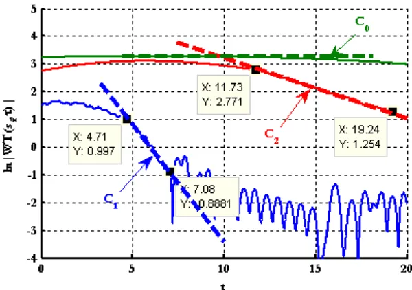
(33) c.e du .au am in@ iam wa in, Am lid Wa. ht. Figure 2.2: (a) Bow vertical acceleration, (b) keel and vertical steel post strain gauges during a severe slamming event showing the time delay of strain gauge peaks from the bow vertical acceleration peak.. Rig. It is quite possible that local stress peaks near the bow could occur before the acceleration peak. However, this occurred for a couple of instances in nearly 100 slams in this run and. py. should not be regarded as a dominant behaviour. Although slamming events are of typically short time application, they need to be more identified in terms of their time. Co. history development which cannot be carried out using conventional signal analysis techniques such as Fourier transform. Frequency analysis of structural response signals reflects the power content of the analysed signal indicating the frequency at which this power is delivered. A typical amplitude. 33.

(34) spectrum generated by the FFT built-in MATLAB function, Math Works [34]and Magrab et al. [35], is shown in Figure 2.3. T2_3. T1_5. T1_8. T1_6. T1_9. T1_7. T1_10. 0.06 0.06 0.05 0.02 -0.29 -0.03 0.07 0.03 0.05 0.04 0.05 0.02 0.01 0.11 0.12 0.04 0.05. 0.01 0.01 0.01 -0.01 0.03 -0.02 0.06 -0.01 -0.01 0.07 0.05 -0.03 0.01 0.04 0.13 0.04 0.09. 0.18 0.18 0.17 0.16 0.08 0.1 0.14 0.14 0.12 0.12 0.03 0.15 0.14 0.14 0.14 0.06 0.02. 0.1 0.1 0.09 0.08 0.17 0.05 0.06 0.05 0.03 0.04 0.14 0.07 0.07 0.05 0.06 0.15 0.01. 0.13 0.13 0.11 0.1 0.03 0.07 0.1 0.08 0.08 0.1 0 0.1 0.1 0.09 0.09 0.03 0.04. 0.04 0.04 0.03 0.03 0.1 0.01 0.03 0.02 0.01 0 0.1 0.02 0.03 0.02 0.02 0.09 0.07. 0.11 0.1 0.03 0.08 0 0.07 0.07 0.06 0.05 0.06 0.14 0.07 0.06 0.06 0.05 0.07 0.13. 0.03 0.02 0.02 0.02 0.07 0.07 0.12 0.02 -0.04 -0.02 0.02 0.13 0.03 0.11 0.04 0.09 0.08. 0.027. 0.027. 0.121. 0.077. 0.081. 0.071. 0.047. in@. am. c.e du .au. T2_2. 0.038. Av delay per event 0.09 0.088 0.07 0.065 0.017 0.035 0.075 0.052 0.047 0.061 0.072 0.057 0.06 0.072 0.087 0.068 0.058. iam. Max Acc time 856.14 415.87 207.12 710.89 565.98 274.1 773.89 29.73 63.260 183.96 117.38 252.71 344.96 592.73 77.15 242.24 725.47 Av delay per gauge. wa. Table 2.2, Average time strain peak delays from bow vertical acceleration peak.. The spectrum of the bow vertical acceleration shows three main frequency components at. in,. 0.2, 0.4 and 2.5 Hz. The first two peaks represent the wave load response frequency while. Am. the third would be a higher mode of excitation probably due to slamming. The spectrum of the strain gauge T1_9 shows four peaks at 0.2, 1.5, 2.2 and a narrow single peak at 0.6 Hz, Figure 2.4. It can be seen that both spectra agree on the underlying wave response. lid. frequency of 0.2 Hz. Considering the locations of both sensors (the accelerometer was. Wa. located on the ship’s centreline while the strain gauge was located on the starboard side) the 1.5 Hz peak appears only on the strain gauge record raising a strong possibility that this. ht. could be the pitch torsional response frequency when the ship sustained a loading. Rig. asymmetry. However, this is not the case as will be shown later in Section 5.2.2. Another spectral component exists in the bow vertical acceleration record, Figure 2.3, close to the value of 1.5 of gauge T1_9, however, it is very weak and is not clear enough to be regarded. py. as a spectral component. Interpretation of the spectral component is therefore difficult and. Co. requires previous knowledge about the structure vibration modes. This may be done experimentally, or by using FE modal analysis. Although the amplitude spectrum gives valuable information on the dominant frequencies of the response signal, it should be noted that this is absolutely correct only if the signal is stationary. A drawback to this rule is that slamming events are smeared, distributed along. 34.

(35) the frequency axis and cannot be isolated as individual events. Also, all time information regarding specific slamming events is lost. A possible solution is to introduce the concept of Windowed Fourier Transform, WFT, or. c.e du .au. Short Time Fourier Transform, STFT, Gabor [36]. The difficulty within this concept is the definition of a window width which is suitable for the whole record. This procedure cannot be easily applied for the current application. For example: it would have difficulty distinguishing two consecutive slamming events without a clear separation in the time domain. Figure 2.5 shows the interference between two consecutive slam events at the. am. instants 274.09 and 278.74 s. The instant of the first slam’s end and the instant of the. in@. second slam’s start cannot be defined accurately.. Hence, traditional signal analysis in either time or frequency domains are not sufficient to. iam. explore the characteristics of slamming events. A better understanding can be achieved if both time and frequency are explored simultaneously which is offered by the wavelet. Co. py. Rig. ht. Wa. lid. Am. in,. wa. analysis which can describe the signal in the time-frequency space.. 35.

(36) c.e du .au am in@ iam wa in, Am lid Wa ht Rig py Co. Figure 2.3: Amplitude spectrum in (g’s)2 of bow vertical acceleration signal.. 36.

(37) c.e du .au am in@ iam wa in, Am lid Wa ht Rig py Co. Figure 2.4: Amplitude spectrum in (µ strain)2 of T1_9 strain gauge (amidships, keel CG) signal.. 37.

(38) 2.3.1. Time series representation in time-frequency space. Spectral analysis by Fast Fourier Transform, FFT, represents an appropriate tool for exploring the energy content of a signal in the frequency domain. Unfortunately, non-. c.e du .au. stationary signals like slamming would lose all time information in such an analysis which is of extreme importance in slamming occurrence prediction. Although the frequency domain provides valuable outcomes, it is meaningless without information about the required time for this frequency to occur. In other words, it is more convenient to define a frequency component and its corresponding time of occurrence. Unfortunately, this. am. cannot be determined accurately according to the Heisenberg Uncertainty theorem as applied to signal analysis. The principal was first defined in the field of quantum mechanics. in@. by Heisenberg [37] stating "The simultaneous determination of two related quantities, for example the position and momentum of a particle, has an unavoidable uncertainty". This. iam. uncertainty is not related to the measuring means or devices but the physical nature of the. Rig. ht. Wa. lid. Am. in,. wa. measured quantities.. Figure 2.5: Interference between consecutive slams, SG T1_9, Run H1_59.. py. For any signal represented in the time domain, the frequency and time characteristics. Co. follow the same principle. In other words, it is impossible to define a frequency and its corresponding time of occurrence simultaneously, Polikar [38], simply because a time interval is needed to define a frequency. Instead, a band of frequencies can be known during a time interval. FFT describes explicitly the frequency components of a signal on the basis of time information which means that FFT cannot be used to analyse nonstationary signals in which the localization of transients is of extreme importance.. 38.

(39) To overcome this problem, the Short Time Fourier Transform STFT has been introduced by Gabor [36], in which the time record is divided into equal size windows. For each of these windows, an FFT is applied to extract the frequency components within the. c.e du .au. predefined window. However, lower frequency signal components, which correspond to a wider time frame may not be identified within the specified window borders. Window size optimisation is necessary to obtain the best representation of the frequency content in the signal. Narrow windows give more precision about time information but less about frequency and vice versa. Wavelet transforms solve this dilemma by presenting the signal. am. frequency content in frequency bands. Narrow time windows are used to resolve high frequency components while wider windows are used to resolve low frequency. in@. components. Figure 2.6 (a) and (b) show that windowed Fourier transform cannot achieve good resolution for both time and frequency simultaneously. Good frequency resolutions. iam. can only be obtained using wider time windows, while the wavelet analysis permits the. Wa. lid. Am. in,. wa. change of window size according to the target frequency band.. 2.3.2. Rig. ht. Figure 2.6: Time-frequency resolution; (a) narrow window STFT gives better time resolution, (b) wider window improves frequency resolution, and (c) wavelet transform changes window size according to the target frequency band, Mallat [39].. Continuous wavelet transform. py. The continuous wavelet transform turns a signal f ( t ) into a function with two variables;. Co. scale and time which are called the wavelet transform coefficients, Hubbard [40], by applying an inner product for the analysed signal f ( t ) and "daughter" wavelets that are generated from a "mother" wavelet by dilation (scaling or stretching) and translation (or shifting) along the time axis. The inner product of these functions can be interpreted as the projection of the daughter wavelet onto the signal f ( t ) or a correlation between the daughter wavelets and the signal f ( t ) at time t . The mother wavelet function is a pre-. 39.

(40) defined function within a finite domain characterised by oscillation. It can be a real or a complex function. The scale parameter is a real number which results in dilation of the mother wavelet so that the resulting wavelet resembles the mother but at a different central. c.e du .au. frequency and/or bandwidth. The translation parameter is a real number which results in the translation or shifting of the wavelet in the time domain. The inner product result is a real or complex number that reflects how close the wavelet frequency is compared to the frequency of f ( t ) at a given location along the time axis. 2.3.2.1. Mathematical background. am. A detailed mathematical background of wavelets, which is beyond the scope of the present. in@. work, can be found in Grossmann et al. [41], Daubechies [42], Kaiser [43], Jorgensen et al. [44], Farge [45], Delprat et al. [46], Mallat et al. [47], Rioul et al. [48], Torrence et al. [49]. iam. and Polikar [50]. A brief mathematical introduction that can be summarized as follows: The "daughter" wavelets are generated by shifting and dilating a "mother" wavelet function. 1  t −τ ψ s  s. in,. ψ s ,τ ( t ) =. wa. ψ (t ).   , s , τ ∈ R , s ≠ 0. . (2.1). Am. where s is the scale parameter and τ is the translation parameter and R is the positive real. Wa. lid. number subset. The wavelet transform of function f ( t ) is defined as: ∞. WT ( s ,τ ) =. ∫. f ( t ).ψ s ,τ dt ,. (2.2). −∞. WT ( s , τ ) =. s 2π. ∞. ∫. fˆ (ω ) ψˆ ( sω ) e iωτ d ω ,. (2.3). −∞. py. Rig. ht. Or in terms of the Fourier transform fˆ (ω ) of function f ( t ) :. Co. where ψ s ,τ is the conjugation of ψ s ,τ and “^” denotes the Fourier transform. If the function ψ is almost zero outside a certain neighbourhood in the time domain, then Equation (2.2) proves that the transform WT ( s , τ ) depends only on the values of f ( t ) in this neighbourhood. Similarly, if ψ is insignificant far from a central frequency (or a frequency band), then Equation (2.3) proves that the transform. WT ( s , τ ) reveals the. properties of fˆ (ω ) in the neighbourhood of this central frequency, Mallat [39].. 40.

(41) A function ψ can be regarded as a wavelet if it satisfies the following conditions: 1- The function has a finite energy ( < ∞ ). Most researchers (e.g. Salimath [51], Jordan et al. [52], Smith [53], Abid et al. [54], Thiebaut et al. [55], Antonie et al. [56], andAnant [57]). c.e du .au. agree on this condition while Kumar et al. [58], Torrence et al. [49], Senhadji et al. [59], and Plett [60]recommended that the mother wavelet has a unit energy; i.e., ∞. ∫ ψ (t ). 2. dt = 1.. −∞. (2.4). am. This condition implies the continuity and smoothness of the mother wavelet and its. in@. daughters.. 2- The function has compact support (limited domain) or sufficiently fast decay to obtain. iam. localisation in time (or space).. wa. 3- The function has compact support in the frequency domain which vanishes at ω ≤ 0. in,. 4- The function has a zero mean; the admissibility condition ∞. ∫ ψ ( t )dt = 0.0,. Am. (2.5). −∞. lid. or ∞. 2. Wa. ψˆ (ω ) ∫ ω d ω = const . = Cψ / 2π < ∞. −∞. (2.6). ht. The admissibility condition implies that the Fourier transform of ψ is rapidly decreasing. Rig. near ω = 0 . Therefore, the Fourier transform of the daughter wavelets forms a bank of band-pass filters with constant ratio of width to centre frequency, Farge [45] and Antonie. py. et al. [56]. The admissibility condition guarantees energy preservation according to. Co. Parseval's theorem, Rade et al. [61]. This means that the energy of the analysed signal can be related to the transformed signal, Perrier et al. [62], through: ∞. ∫. −∞. 2. f ( t ) dt =. 1 Cψ. ∞ ∞. ∫∫. WT ( s ,τ ). 0 −∞. 41. 2. dsdτ 1 = 2 2π s. ∞. ∫. −∞. 2 fˆ (ω ) d ω . (2.7).

(42) It is surprising that there is no consistency among researchers in representing the wavelet transform. The most popular are the scalograms, the wavelet power spectrum, and the global wavelet spectrum. No single definition can be found for these three representations. In summary, the. c.e du .au. wavelet transform is presented graphically as follows: 1- The "wavelet scalogram" is a two-dimensional image or contour plot in which the abscissa represents the translations (time) and the ordinate represents the scales or frequencies. The colour map, or the contours, represents the wavelet transform coefficient, Liu [63], Goelz et al. [64] and Jordan et al. [52]. In the case of complex transforms, a real, imaginary,. am. modulus and phase scalograms may be introduced, Misiti et al. [65]. Squaring of the. in@. transform coefficients has the advantage of increasing the contrast between large and small values which enables better interpretations, Kumar et al. [58]and Plett [60].. iam. 2- The "wavelet spectra" or "wavelet energy spectrum" where the time-scale energy density is. wa. defined by Farge [45] and is given by:. 2. WT ( s , τ ) E( s , τ ) = . s. in,. (2.8). The wavelet spectra is represented as a contour or image plot. The reason behind the. Am. division by the scale is to normalize all the band-pass filters so that they have the same. lid. peak, Jordan et al. [66]. Perrier et al. [62] expressed the local spectrum as:. 1 ω 2 WT ( s ,τ ) , s = o , ω ≥ 0, ωo = 2π f c , Cψ .ωo ω. (2.9). Wa. E( s , τ ) =. ht. where ωo and ω represent the mother wavelet's and daughter wavelet's wave numbers. Rig. respectively in radians. fc is the mother wavelet's central frequency in Hz. According to Equation (2.9), the local spectrum measures the contribution to the total. py. energy coming from the vicinity of point t and wave number ω , this vicinity depends on. Co. the shape in time and frequency space of the mother wavelet, Perrier et al. [62]. 3- The "global wavelet spectrum" is defined as the energy content within each scale and is expressed as:. 2. WT ( s , τ ) E( s ) = ∫ E( s ,τ )dτ = ∫ dτ . s R R. 42. (2.10).

(43) The "global wavelet transform" or "mean wavelet transform", as named by Perrier et al. [62], can be expressed as: 2. ∞. ∞ WT ( s , τ ) 1 E( s ) = WT ( s ,τ ) dτ = dτ . (2.11) ∫ ∫ 2Cψ .ωo −∞ 2Cψ ω −∞ s. 2. c.e du .au. 1. The factor of 1/2 was initiated based on the energy definition by Perrier et al. [62] as 1 2 f ( t ) dt in comparison to Farge [45] definition as ∫ 2. ∫. 2. f ( t ) dt . The "mean wavelet. ∞. 1. E(ω ) ψˆ ( sω ) Cψ ω ∫. 2. in@. E( s ) =. am. spectrum" can then be related to the Fourier spectrum through, Perrier et al. [62],:. 0. dω,. (2.12). iam. where ψˆ is the Fourier transform of the daughter wavelet at scale s and E(ω ) is the Fourier spectrum. The global wavelet spectrum as defined by Farge [45] can also be related to. wa. the Fourier transform of the analysing function as:. 2. E( s ) = ∫ E(ω ) ψˆ ( sω ) d ω .. in,. (2.13). R. ∞. Am. Combining Equations(2.11), (2.12) and (2.10), (2.13) we can write:. 2. ∞. lid. ∫ E(ω ) ψˆ ( sω ) d ω = ∫ 0. (2.14). Wa. 0. 2. WT ( s , τ ) dτ . s. Equation (2.14) shows that the wavelet spectrum resembles a weighted average of the. ht. Fourier spectrum by the square of the Fourier transform of the scaled analysing wavelet, Farge [45], Thiebaut et al. [55], Perrier et al. [62], Roques et al. [67], and Christopoulou et. Rig. al. [68].. Co. [45]:. py. 4- The "local energy spectrum" is defined as the temporal energy density and is given by Farge. E(τ ) =. 1 Cψ. ∞. ∫ E( s ,τ ) 0. ∞. ds WT ( s ,τ ) = Cψ−1 ∫ ds . 2 s s 0. (2.15). In the current study, the "wavelet energy spectrum" and "global wavelet spectrum" as defined in Equations (2.8) and (2.10) are used in wavelet transform representations based on the linkage to Fourier transform as indicated in Equation(2.14).. 43.

No results found