An Optimizing Method for Screening in A Mixture Design Experiment

Rochester Institute of Technology

RIT Scholar Works

Theses Thesis/Dissertation Collections

12-2017

An Optimizing Method for Screening in A Mixture

Design Experiment

Marcos Michael Soriano Almanzar

[email protected]

Follow this and additional works at:https://scholarworks.rit.edu/theses

This Thesis is brought to you for free and open access by the Thesis/Dissertation Collections at RIT Scholar Works. It has been accepted for inclusion in Theses by an authorized administrator of RIT Scholar Works. For more information, please [email protected].

Recommended Citation

An Optimizing Method for Screening in A Mixture Design

Experiment

by

Marcos Michael Soriano Almánzar

A thesis submitted in partial fulfillment of the requirement for

the Degree of Master of Science in Applied Statistics

Department of Applied Statistics

College of Science

Rochester Institute of Technology

Rochester Institute of Technology

College of Science

Master of Science in Applied Statistics

Thesis Approval Form

Student Name: Marcos Michael Soriano Almánzar

Thesis Title: An Optimizing Method for Screening in A Mixture Design

Experiment

Thesis Committee

Name Signature Date

Dr. Robert Parody

Thesis Advisor

Dr. Ernest Fokoue

Committee member

iii

Abstract

iv

Acknowledgments

v

Contents

1. Mixture Experiments ... 1

2. Pseudo-components ... 4

3. Ridge plots ... 9

4. Related work ... 11

4.1. Screening design ... 11

4.2. Component effect ... 12

5. Methodology ... 14

6. Examples ... 16

6.1. Motor octane example ... 16

6.2. Waste glass example ... 20

7. Discussion ... 24

8. Conclusion ... 25

9. Reference ... 26

vi

List of Tables

Table 1 Upper bound example ...7

Table 2 Motor octane example; experimental design with results ... 17

Table 3 Estimated Angles for Example 1 ... 19

Table 4 Angles with 95% Confidence Bounds for Example 1 ... 19

Table 5 Component restriction ... 20

Table 6 Estimated Angles for Example 2 ... 22

Table 7 Angles with 95% Confidence Bounds for Example 2 ... 23

vii

List of Figure

Figure 1 . Lower bound simplex ... 5

Figure 2 Upper bound simplex ...7

Figure 3 Lower and Upper bound simplex ... 8

Figure 4 first degree trace plot ... 9

Figure 5 second degree trace plot ...10

Figure 6 Ridge plot 1 ... 18

1

1.

Mixture Experiments

Mixture experiment is a type of experiment where the responses is subject to the proportion of the components in the mixture and not on the total amount of the mixture. For example, the response might be the mileage of the blend of gas or the flavor of a fruit punch juice. Looking at the examples above we can notice that the response is going to depend in how much we add from each of the component. In a mixture experiment, the q components satisfy the following constraints:

x_i ≥ 0, i = 1,2,3, … , q and ∑q_i=1x_i = x₁+ x₂+ ⋯ + x_q = 1 (1.1)

Since the proportion of the component must be between 0 and 1 and the proportions of the q components in the mixture must sum to one. The constrain show in Eqs. (1.1) the experimental region of the factor space containing the component consist of a regular (q − 1)-dimensional simplex. For (q = 2) component the region is a straight line, for (q = 3) component the region is a triangle, for (q = 4) component the region is a tetrahedron and so on.

2

x_i = 0,1

m, 2

m, … , 1 (1.2)

And the [q,m] simplex lattice consist of all possible combination of the component where the proportions (1.2) for each component are used. For example, in a 3 component system lets assume the proportion 𝑥_𝑖 = 0,1

2, 1 for i=1,2 and 3. Setting m=2 for the proportion in equation (1.2), the [3,2] simplex

lattice consist of the six points on the boundary of the triangle.

(𝑥_𝑖, 𝑥_𝑖, 𝑥_𝑖) = (1,0,0), (0,1,0), (0,0,1), (1 2,

1 2, 0) , (

1 2, 0,

1 2) , (0,

1 2,

1 2)

The number of the design points in the [q,m] simplex lattice is (q+m−1_m ). In the [3,2] simplex lattice for example the number of points is (3+2−1₂ ) = 6.

A general form of regression function that can be fitted to data collected at the points of a [q,m] simplex lattice is derived as follow

n= β₀+ ∑q_i=1β_ix_i+ ∑q_i<jβ_ijx_ix_j+ ⋯ (1.3)

The number of term in Eq. (1.3) is (q+m_m ) , but because the term in Eq. (1.3) have meaning for us only subject to the restriction x₁+ x₂+ ⋯ + x_q= 1, we know that the betas associates with the terms are not unique, but, we are going to substitute

3

In Eq.(1.3) to remove the dependency among the xi terms, doing this n becomes a

polynomial of degree m in q-1 components x1 + x2+ ⋯ + xq−1 with (q+m−1_m ) terms. Now the bad

thing doing this is that the effect of the component q because is not included in the equation. An alternative is multiplying some term in Eq. (1.3) by the identity (x₁+ x₂ + ⋯ + x_q) = 1 and simplifying. The resulting equation is called the canonical polynomial, the number of terms in the [q,m] polynomial is (q+m−1_m ) and this number is equal to the number of points that make up the associated [q,m] simplex lattice design. For example, for m=1

n = β₀ + ∑ β₁x₁

q i=1

And multiplying the β0 term by (x1+ x2+ ⋯ + xq) = 1 the resulting equation is

n = β₀(∑q_i=1x_i) + ∑_i=1q β₁x₁ = ∑q_i=1β_i∗x_i (1.5)

Where β_i∗ = β0+ β1 for all i=1,2,…,q.

For the mixture design, we usually want to fit a quadratic model of the form

4

The mixture at the vertices of the simplex are known as pure component blends, this is a 100% mixture of the single factor assigned to each vertex. All blends along each side of the simplex are binary component blends. The interaction terms in the model are denoted to as non-linear blending terms. We have two types of non-linear blending, synergistic when the response is greater than the predicted linear response and antagonistic when response is lower than the predicted linear response.

Scheffé continued his pioneering work in the field with the introduction of the Simplex Centroid design. This design contains 2q − 1 mixtures containing q pure component blends, q binary blends with equal proportions, and q ternary blends with equal proportions up to the q-nary mixture with equal proportions. Similarly, with the Simplex-Lattice designs, the Simplex-Centroid design has a one-to-one correspondence with the Scheffé polynomial and the coefficients can be estimated utilizing linear combinations of the responses at each of the design points.

2.

Pseudo-components

The ‘pseudo’ component are defined as combinations of the original components and the primary reason for introducing the pseudocomponents is that usually both the construction of design and the fitting of models are more easier when done in the pseudocomponents system than when done in the original component system.

When we have additional constrain on the component proportion whether is bases on a lower bound, upper bound or both then we ended written as 0 ≤ 𝐿𝑖 ≤ 𝑥𝑖 ≤ 𝑈𝑖 ≤ 1 𝑓𝑜𝑟 𝑖 = 1,2,3, … , 𝑞.

5

When we are in presence of a lower bound 𝐿𝑖 ≥ 0 𝑓𝑜𝑟 𝑖 = 1,2, … , 𝑞 then we use what is

call L-pseudo-component where 𝑥′𝑖 is defined using the linear transformation and 𝐿 = ∑𝑞𝑖=1𝐿𝑖 <

1

𝑥′𝑖 = (𝑥𝑖−𝐿𝑖)

1−𝐿 , 𝑓𝑜𝑟 𝑖 = 1,2, … , 𝑞 𝑎𝑛𝑑 𝐿 < 1 (2.1)

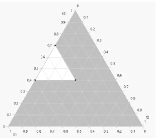
Assume that 𝑞 = 3 with a component constrains of 𝑥1 ≥ 0.3, 𝑥2 ≥ 0.4 𝑎𝑛𝑑 𝑥3 ≥ 0.3.

Figure 1 show the resulting simplex. The experimental region is still a triangle, but is much smaller now.

6

Once the mixture blends in the original system are defined from the L-pseudocomponet setting, the next step is to collect observed values of the response at the design so that a model can be obtained. A second degree polynomial L-pseudocomponent is

𝑛 = 𝛾1𝑥′1+ 𝛾2𝑥′2+ 𝛾3𝑥′3+ 𝛾12𝑥′1𝑥′2+ 𝛾13𝑥′1𝑥′3+ 𝛾23𝑥′2𝑥′3

When one or more of the component proportions is restricted by upper bound 𝑥_𝑖 ≤ 𝑈, the simplest modification to the simplex lattice design is replacing the restricted component with mixture consisting in combinations of the restricted component and predetermined proportion of the unrestricted component.

Now when we are in presence of an upper bound 𝑈_𝑖 ≤ 1 𝑓𝑜𝑟 𝑖 = 1,2, … , 𝑞 Crosier (1984) defined what is call U-pseudo-component where 𝑥′_𝑖 is defined using the linear transformation and

𝑢 = ∑𝑞𝑖=1𝑈𝑖 > 1

𝑥′_𝑖 =(𝑈𝑖−𝑥𝑖)

𝑈−1 , 𝑓𝑜𝑟 𝑖 = 1,2, … , 𝑞 𝑎𝑛𝑑 𝑈 > 1 (2.2)

The new region now is an inverted triangle and in some cases the vertices may extend beyond the original experimental region and will not meet the restriction in (1). To test this, we will see if

𝑈 − 𝑈_𝑚𝑖𝑛 < 1, (2.3)

7

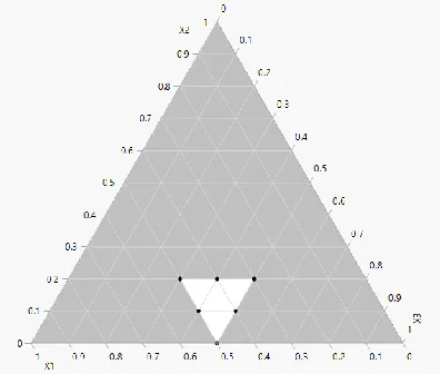
When (2.3) is met, then the experimental region lies entirely inside the original region. When (2.3) is not met then we have to constrain the experimental region to points that fall in the intersection between the original experimental region and the restricted region. Here we show two examples where the components are restricted just by upper bounds.

Based on table 1, we can see that for example 1 that the entire restricted region is inside the simplex but that is not the case for example 2.

Table 1 Upper bound example

example bounds 𝑼 − 𝑼𝒎𝒊𝒏

1 𝑥₁ ≤ 0.5, 𝑥₂ ≤ 0.2 𝑎𝑛𝑑 𝑥₃ ≤ 0.5 1.0

2 𝑥₁ ≤ 0.4, 𝑥₂ ≤ 0.8 𝑎𝑛𝑑 𝑥₃ ≤ 0.7 1.5

8

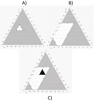
In the general case where we a present with both lower and upper bound restriction the resulting region is just the intersection of the two individual regions. The boundaries of the constrained region 0 ≤ 𝐿_𝑖 ≤ 𝑥_𝑖 ≤ 𝑈_𝑖 ≤ 1 𝑓𝑜𝑟 𝑖 = 1,2,3, … , 𝑞 that are to be used for the design depends on the form or degree of the equation that is to be used to model the surface over the region. Much of the time we are required for our design point location at least some of the extreme vertices of the region as well as midpoints and centroids of some of the edges and two dimensional faces of the region. For example, let’s assume that the component is 0.3 ≤ 𝑥1 ≤ 0.8, 0.4 ≤ 𝑥2 ≤

0.6 𝑎𝑛𝑑 0.15 ≤ 𝑥₃ ≤ 0.3. The plot both the lower and upper simplexes are show in figure 3.

Figure 3 Lower and Upper bound simplex

A)

C)

9

3.

Ridge plots

Ridge plots are graphs that show values of the estimated response while moving away from the centroid of the simplex experimental area. With this type of graph, we can examine the effect that each component has on the response and see which components are the most

influence.

This type of graph is very useful when we have 4 or more components in the mixture and we cannot visualize the response Surface on a contour plot because of the dimension. In order to graph we will use what is known as "cox's direction" introduced by Cox (1971) which is an alternative model to the Scheffé model to measure the effects of the components when we have an increase in the proportion Δ_i in component i.

When 𝑥_𝑖 is changed to 𝑥_𝑖 + ∆_𝑖, 𝑥_𝑗 is changed to 𝑆_𝑗− ∆_𝑖𝑠_𝑗/(1 − 𝑠_𝑖), For 𝑗 = 1,2, … , 𝑖 − 1, 𝑖 + 1, … , 𝑞, 𝑤ℎ𝑒𝑟𝑒 𝑠 = (𝑠₁, 𝑠₂, … , 𝑠_𝑞) is some reference mixture.

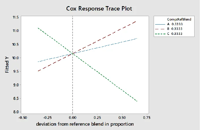
The following plot show for a 3 component show how a first-degree model looks like, as we can see the they are straight line

10

Now the same experiment but in here we are fitting a second-degree model, the trace plot are curves for each of the component.If the curve almost flat means that the changes along Cox’s direction and other components keep the same ratio and the response don’t change to a great extent.

11

4.

Related work

4.1.

Screening design

industries many times there is present a large number of component, at least more than 6 of potentially important component that can be considered candidates in an experiment.

First the strategy is to know from all the potentially important component which ones are the ones that are the most important so in order to do it we need to run an experiment and decide the most important component from the size of their effect.

The construction of screening design and the setting up of screening models quite often begin with the Scheffé first degree model:

𝑛 = 𝛽1𝑥1+ 𝛽2𝑥2+ 𝛽3𝑥3+ ⋯ + 𝛽𝑞𝑥𝑞 (4.1)

An essential component may be a single one or the sum of two or more components and we can find them looking if they don’t have any effect and/or have equal effect. We have two types

i) If a coefficient 𝛽̂𝑖 is equal to the average of the remaining coefficient in the model, then

there is no variation in Y along any line perpendicular to the 𝑥𝑖 = 0 base of the simplex.

This is the one-dimensional subspace of the simplex in which 𝑥_𝑖 = 1−𝑥𝑖

𝑞−1 for all 𝑗 ≠ 𝑖.

ii) If two or more coefficients are equal for example 𝛽̂1 = 𝛽̂3 = 𝛽̂5 then the associated

12

We normally use an Axial design to set up the experiment. This are designs that consist mainly of q component where all the points are inside the simplex and follows the axial lines. By definition the axis of component i is the imaginary line extending from the base point 𝑥_𝑖 = 0,

𝑥_𝑗 = 1

𝑞−1 for all 𝑗 ≠ 𝑖, to the vertex where 𝑥𝑖 = 1, 𝑥𝑗 = 0 for all 𝑗 ≠ 𝑖. Usually, points located at

the half distance from the overall centroid to the vertex are called axial points/blends.

4.2. Component effect

When we are measuring the component effect we can choose a reference mixture to be the centroid of the constraint region and allow us to incorporate both shape and location information into the measure. The basic strategy for developing a new direction in which to compute effects will be to transform to pseudocomponents and then apply 𝑥_𝑖 − ∆_𝑖𝑠_𝑖/(1 − 𝑠_𝑖), where the reference mixture is taken to be the centroid of the constrain region. This direction is determined by the line joining the centroid of the constrain region to the pseudocomponents simplex.

The total effect of the component i may be measure as the difference of predicted response values 𝑇𝐸𝑖 = 𝑦̂(𝑥𝐻) − 𝑦̂(𝑥𝐿) (4.2)

Where 𝑥𝐻 and 𝑥𝐿 are points in th constrain refion such that the component i is the highest and

lowest values respectively. The points 𝑥_𝐻 and 𝑥_𝐿 will depend on the restriccion of the form (1.1) and from the restriction of the Upper and Lower bounds.

13

𝐸_𝑖 = 𝛽̂_𝑖 − (𝑞 − 1)−1∑𝑞_𝑗≠𝑖𝛽̂_𝑗 (4.3) 𝐸𝑖 = 𝑅𝑖[𝛽̂𝑖 − (𝑞 − 1)−1∑𝑞𝑗≠𝑖𝛽̂𝑗] (4.4)

𝑤ℎ𝑒𝑟𝑒 𝑅𝑖 = 𝑏𝑖− 𝑎𝑖

They also noted that cox work and listed the following formula for the total effect of the component i relative to a reference mixture s:

𝐸_𝑖 = ( 𝑅𝑖

1−𝑠𝑖) (𝛽̂𝑖 − ∑ 𝛽̂𝑗𝑠𝑗

𝑞

𝑗=1 ) (4.5)

The inherent direction in which the effect is measured is determined by the line joining the reference mixture and the ith component simplex vertex.

Piepel defined a new direction that is closely related to Cox direction to calculate the total and partial effects. The new direction is defined in a L-pseudocomponent system like we explain in chapter 2. Using only the lower bound 𝐿_𝑖, i=1,2,3,…,q. this region is simplex with vertices defined by where 𝑥_𝑖 = 1, 𝑥_𝑗 = 0 for all 𝑗 ≠ 𝑖.

Now the total effect (4.2) of the component i is obtained by substituting the range 𝑅𝑖, or using the

14

5.

Methodology

Now, in this new method we are interested in the angle because, it doesn’t matter if the line is inside or outside the experimental region we always are going to get the same angle. To get the angle what we are interested is to get the ratio between the amount of change 𝑦 ∆_𝑦 vs the amount of change of 𝑥 ∆𝑥.

Because we are dealing with constrained designs we are going to produce coefficients which are highly correlated, so we must use Pseudo-components to simplify design construction and model fitting, and reduce the correlation between component bounds.

Also, we are assuring that no matter what the experimental region looks like we can get the end point of the reference line by doing the transformation and don’t need to worry about if the line is outside the experimental region.

To obtain what we are interested in, first we must calculate our ∆𝑥. Normally that is going to

be equal to:

∆_𝒙= ∆_𝒊 = (𝑹_𝒊− 𝒔_𝒊), 𝑤ℎ𝑒𝑟𝑒 𝑅 𝑖𝑠 𝑡ℎ𝑒 𝑟𝑎𝑛𝑔𝑒 𝑜𝑓 𝑥 𝑎𝑛𝑑 𝑠 𝑖𝑠 𝑡ℎ𝑒 𝑟𝑒𝑓𝑒𝑟𝑒𝑛𝑐𝑒 𝑙𝑖𝑛𝑒 (5.1)

But because we transform into pseudocomponents our ∆_𝑥 now become the following:

∆_𝑥= 1 −1

𝑞 , 𝑤ℎ𝑒𝑟𝑒

1

15

Next to obtain or ∆_𝑦 we first need to get our responses 𝑌_𝑖 = 𝑥_𝑗′𝛽̂ and then from there we take the maximum and the minimum for each component, so we will end with:

∆_𝒚= |𝐦𝐚𝐱 (𝒀_𝒊) − 𝐦𝐢𝐧 (𝒀_𝒊)| (5.3)

Now that we have our deltas then we can proceed to take the absolute value of the ratio.

𝑹𝒂𝒕𝒊𝒐 =∆𝒚

∆𝒙 (5.4)

To obtain our angle 𝜃 we must the take arctan of the ratio.

𝜽 = 𝐚𝐫𝐜𝐭𝐚𝐧(𝑹𝒂𝒕𝒊𝒐) = 𝐚𝐫𝐜𝐭𝐚𝐧 (∆𝒚

∆𝒙) (5.5)

We can make a ∆_𝑦 (1 − 𝛼)𝑥100% 𝑐𝑜𝑛𝑓𝑖𝑑𝑒𝑛𝑐𝑒 𝑖𝑛𝑡𝑒𝑟𝑣𝑎𝑙 𝑓𝑜𝑟 𝑡ℎ𝑒 𝑎𝑛𝑔𝑙𝑒 then the interval is

𝐚𝐫𝐜𝐭𝐚𝐧 [𝑹𝒂𝒕𝒊𝒐 ± [𝒕_𝒇,𝜶

𝟐] √𝒗𝒂𝒓

̂ [𝒚̂(𝒙)]] (5.6)

Where 𝑓 is the number of degrees of freedom is associated with the sample estimate 𝑠2 to estimate𝜎2_{, and 𝑡}

𝑓,𝛼

2

is the tabled t-value with 𝑓 degrees of freedom at a 𝛼/2 level of significance.

16

6.

Examples

6.1.Motor octane example

The first example is an experiment to give the reader an idea of the practicality of this technique. In this experiment the motor octane rating from 12 different blends were recorded to determine the effect of the following gasoline-blending component within the specified ranges. The response, y, for this experiment is Motor Octane at 1.5 mL Pb/gal

𝑆𝑡𝑟𝑎𝑖𝑔ℎ𝑡𝑟𝑢𝑛 (𝑥1): 0 ≤ 𝑥1 ≤ 0.21

𝑅𝑒𝑓𝑜𝑟𝑚𝑎𝑡𝑒 (𝑥₂): 0 ≤ 𝑥₂ ≤ 0.62

𝑇ℎ𝑒𝑟𝑚𝑎𝑙𝑙𝑦 𝑐𝑟𝑎𝑘𝑒𝑑 𝑛𝑎𝑝ℎ𝑡ℎ𝑎 (𝑥₃): 0 ≤ 𝑥₃ ≤ 0.12

𝑐𝑎𝑡𝑎𝑙𝑦𝑡𝑖𝑐𝑎𝑙𝑙𝑦 𝑐𝑟𝑎𝑐𝑘𝑒𝑑 𝑛𝑎𝑝ℎ𝑡ℎ𝑎 (𝑥₄): 0 ≤ 𝑥4 ≤ 0.62

𝑝𝑜𝑙𝑦𝑚𝑒𝑟 (𝑥5): 0 ≤ 𝑥5 ≤ 0.12

𝑎𝑙𝑘𝑦𝑙𝑎𝑡𝑒 (𝑥₆): 0 ≤ 𝑥₆ ≤ 0.74

𝑛𝑎𝑡𝑢𝑟𝑎𝑙 𝑔𝑎𝑠𝑜𝑙𝑖𝑛𝑒 (𝑥₁): 0 ≤ 𝑥₇ ≤ 0.08

17

Table 2 Motor octane example; experimental design with results

x1 x2 x3 x4 x5 x6 x7 y

0 0.23 0 0 0 0.74 0.03 98.7 0 0.1 0 0 0.12 0.74 0.04 97.8 0 0 0 0.1 0.12 0.74 0.04 96.6 0 0.49 0 0 0.12 0.37 0.02 92 0 0 0 0.62 0.12 0.18 0.08 86.6 0 0.62 0 0 0 0.37 0.01 91.2 0.17 0.27 0.1 0.38 0 0 0.08 81.9 0.17 0.19 0.1 0.38 0.02 0.06 0.08 83.1 0.17 0.21 0.1 0.38 0 0.06 0.08 82.4 0.17 0.15 0.1 0.38 0.02 0.1 0.08 83.2 0.21 0.36 0.12 0.25 0 0 0.06 81.4 0 0 0 0.55 0 0.37 0.08 88.1

This experiment can be found in Cornell, pp. 248. He determined that because of some variance issues, the best results could be found by combining(𝑥₁+ 𝑥₃+ 𝑥₇), creating one component.

The five-term model, fitted to the 12 motor octane rating values, is

𝑦̂(𝑥) = 78.4(𝑥1+ 𝑥3+ 𝑥7) + 85.7(𝑥2) + 81.6(𝑥4) + 88.9(𝑥5) + 101.9(𝑥6)

18

Figure 6 Ridge plot 1

Now based in Figure 4 it seems that components 4, 6 and combination of

19

Table 3 Estimated Angles for Example 1

Based on the estimates, it seems that 𝑥₂ and 𝑥₅ may not be needed given that their angles are approximately 14 and 1.5 respectively.

Now we can employ the method from section 3 to make inference in this situation. Utilizing a critical value of t=2.364 with df=7 and alpha=0.05, we use (eq12) to calculate the 95% confidence intervals for the angles. These results are in Table 4.

Table 4 Angles with 95% Confidence Bounds for Example 1

Component Lower

Bound theta(𝜃)

Upper Bound

𝑥₂ 3.874369 13.701174 22.77593

𝑥4 25.304292 33.938426 41.1243

𝑥₅ -20.59035 1.453238 23.09445

𝑥₆ 50.148909 55.003981 58.91431

𝑥₁+ 𝑥₃ + 𝑥₇ 37.103772 42.890528 47.7652

Based on the results from Table 4, the only component that is not active is 𝑥5. From here it would

be unnecessary to include it in further experimentation. Component theta(𝜃)

𝑥₂ 13.701174

𝑥₄ 33.938426

𝑥5 1.453238

𝑥6 55.003981

20

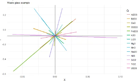
6.2.

Waste glass example

A nuclear waste glass development example with liquidus temperature (TL) of spinel crystals as the response is now presented and used to illustrate the new method. Spinel is a solid solution of trevorite (NiFe2O4) with other oxides (FeO, MnO, and Cr2O3) that forms in nuclear waste glasses with sufficiently high concentrations of Cr, Ni, and Fe. Spinel in sufficient amounts can have an adverse impact on nuclear waste glass melter performance and product glass properties. Hence, spinel TL should be at least 100°C below the nominal operating temperature of a waste glass melter(Hrma et al. [5, 6]). In table 5 we present the component with the following restriction.

Table 5 Component restriction

Component Lower Bound

Upper Bound Al2O3 0.025 0.08

B2O3 0.05 0.1 CaO 0.003 0.02 Cr2O3 0.001 0.003 Fe2O3 0.06 0.15

21

The experimental design with the measured response values are in the appendix in Table 6.

Here again we want to identify all the potentially significant component so if possible try to reduce the number of necessary component to be studied. The ridge trace plot for this example is in Figure 5.

Figure 7 Ridge plot 2

22

centroid of the design as the reference point, which is (1039.396). We then use pseudocomponents to determine ∆𝑥 𝑎𝑠 (1 − 𝑠) . After determining the fitted values 𝑦̂ for the corresponding x-values,

we determine the angles utilizing (eq11). These angles are in Table 7.

Table 6 Estimated Angles for Example 2

Component theta(θ) Al2O3 74.92808

B2O3 69.59915 CaO 66.39033 Cr2O3 89.38641 Fe2O3 82.49851 K2O 75.95145 Li2O 84.36819 MgO 81.8595 MnO 59.69842 Na2O 83.98754 NiO 86.77903 SiO2 8.57424 TiO2 85.68088 U3O8 37.80837

Based on the estimates, it seems that SiO2 and U3O8 may not be needed given that their angles are approximately 8.574 and 37.808 respectively.

23

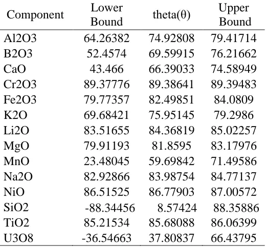
Table 7 Angles with 95% Confidence Bounds for Example 2

Component Lower

Bound theta(θ)

Upper Bound Al2O3 64.26382 74.92808 79.41714 B2O3 52.4574 69.59915 76.21662 CaO 43.466 66.39033 74.58949 Cr2O3 89.37776 89.38641 89.39483 Fe2O3 79.77357 82.49851 84.0809 K2O 69.68421 75.95145 79.2986 Li2O 83.51655 84.36819 85.02257 MgO 79.91193 81.8595 83.17976 MnO 23.48045 59.69842 71.49586 Na2O 82.92866 83.98754 84.77137 NiO 86.51525 86.77903 87.00572 SiO2 -88.34456 8.57424 88.35886 TiO2 85.21534 85.68088 86.06399 U3O8 -36.54663 37.80837 66.43795

24

7.

Discussion

For the motor octane example, we can see that we end up with the same solution as Cornell in which we find a single non-significant component seeing our confidence interval in our analysis. In example number two of the residual glass, we could see that we found some differences between the components that were significant. We saw that in the results of Piepel the components that were not significant were MnO and SiO2 with p values of 0.139 and 0.157 respectively. compared to this new method as we saw earlier we also find two non-significant components, SiO2 and U3O2, the latter being different from one of the components of Piepel MnO. One of the reasons why this could have happened is because Piepel used a different encoding than the one we use.

Analyzing the differences between the new method implemented and the one currently being used, we can see that one of the main advantages of the new method is that we do not have to worry about our reference line being outside the experimental area because we are transforming a pseudocomponents.

Another thing is that in the other methods they are more focused in the parameter estimates, where the larger values of the 𝑏_𝑖, relative to 𝑏_𝑗, 𝑖 ≠ 𝑗, is a component more important. Although the effects of the components are used more to interpret and understand the response Surface determined by the fitted prediction equation, in this new method because we are looking at the angle we don’t need to focus at the estimates, so looking at the angle if we found something that is relatively close to zero then one can infer that the component with that behavior is not

25

8.

Conclusion

We have presented a method for optimizing screening in a mixture design. The idea was to be able to screen to identify all the potentially significant component based on the angles using the ratio of the delta Y and delta X through the use of pseudo components. It can be used in any number of situations for any number of components.

26

9.

Reference

− Cornell, John A. "Some Comments on Designs for Coxs Mixture Polynomial." Technometrics 17, no. 1 (1975): 25.

− Piepel, Gregory F. "Measuring Component Effects in Constrained Mixture Experiments." Technometrics 24, no. 1 (1982): 29.

− Piepel, Gregory F. "Defining Consistent Constraint Regions in Mixture Experiments." Technometrics 25, no. 1 (1983): 97

− Snee, Ronald D. "Experimental Designs for Quadratic Models in Constrained Mixture Spaces." Technometrics 17, no. 2 (1975): 149.

− Snee, Ronald D., and Donald W. Marquardt. "Screening Concepts and Designs for Experiments with Mixtures." Technometrics 18, no. 1 (1976): 19.

− Cornell, John A. "Some Comments on Designs for Coxs Mixture Polynomial." Technometrics 17, no. 1 (1975): 25.

− Cornell, John A. Experiments with mixtures: designs, models and the analysis of mixture data. New Jersey: John Wiley & Sons, 2011.

− H. Scheffe, “Experiments with Mixtures,” Journal of the Royal Statistical Society. Series B (Methodological), vol. 20, no. 2, pp. 344–360, 1958.

− Lambrakis, D. 1963. "Experiments with Mixture: an Alternative to the simplex lattice Design." Journal of the Royal Statistical Society. series B(Methodological) 25 (2): 235-263.

− H. Scheffe, “The Simplex-Centroid Design for Experiments with Mixtures,” Journal of the Royal Statistical Society. Series B (Methodological), vol. 25, no. 2, pp. 235–263, 1963.

− N. R. Draper and W. Lawrence, “Mixture Designs for Three Factors,” Journal of the Royal Statistical Society. Series B (Methodological), vol. 27, no. 3, pp. 450–465, 1965.

− N. R. Draper and W. Lawrence, “Mixture Designs for Four Factors,” Journal of the Royal Statistical Society. Series B (Methodological), vol. 27, no. 3, pp. 473–478, 1965.

27

Quality Control, vol. 22, pp. 592–596, 1966.

− D. Lambrakis, “Experiments with p-component Mixtures,” Journal of the Royal Statistical Society. Series B (Methodological), vol. 30, no. 1, pp. 137–144, 1968.

− 5.5.4.2. Simplex-lattice designs. Accessed October 10, 2017.

http://www.itl.nist.gov/div898/handbook/pri/section5/pri542.htm.

− Weese, Maria, "A New Screening Methodology for Mixture Experiments. " PhD diss., University of Tennessee, 2010. http://trace.tennessee.edu/utk_graddiss/757

28

10.

Appendix

Table 8 Glass waste example; experimental design with results

Glass(a) Al2O3 B2O3 CaO Cr2O3 Fe2O3 K2O Li2O MgO MnO Na2O NiO RuO2 SiO2 TiO2 U3O8

29

SG38 0.025 0.0999 0.003 0.001 0.1464 0.0379 0.03 0.025 0.03 0.1099 0.0005 0.0009 0.4296 0.006 0.0549 897 SG39 0.025 0.0499 0.02 0.003 0.1498 0.015 0.03 0.005 0.03 0.1099 0.02 0.0009 0.5355 0.006 0 1164 SG40 0.0799 0.0999 0.003 0.003 0.0599 0.015 0.03 0.025 0.01 0.1099 0.02 0.0009 0.4826 0.006 0.0549 1173 SG41 0.0799 0.0999 0.02 0.001 0.1499 0.015 0.03 0.005 0.03 0.0599 0.02 0.0009 0.4321 0.0015 0.0549 1304 SG42 0.0448 0.0876 0.0073 0.0025 0.1275 0.0323 0.0524 0.02 0.025 0.0976 0.0054 0.0009 0.4741 0.0049 0.0177 990 SG43 0.0664 0.0876 0.0073 0.0015 0.0825 0.0323 0.0375 0.01 0.025 0.0976 0.0054 0.0009 0.5257 0.0026 0.0177 924 SG44 0.0664 0.0876 0.0073 0.0015 0.1275 0.0208 0.0375 0.02 0.015 0.0726 0.0151 0.0009 0.5052 0.0049 0.0177 1244 SG45 0.025 0.0999 0.02 0.001 0.0599 0.015 0.0299 0.025 0.03 0.1099 0.02 0.0009 0.562 0.0015 0 936 SG46 0.025 0.0499 0.003 0.003 0.1499 0.038 0.0599 0.025 0.01 0.0599 0.02 0.0009 0.4946 0.006 0.0549 1247 SG47 0.025 0.0499 0.02 0.003 0.1499 0.015 0.0599 0.025 0.01 0.1099 0.02 0.0009 0.4551 0.0015 0.0549 1144 SG50 0.025 0.0499 0.02 0.003 0.1499 0.038 0.03 0.005 0.03 0.0599 0.02 0.0009 0.5075 0.006 0.0549 1285 SG51 0.0799 0.0499 0.02 0.003 0.1499 0.038 0.03 0.005 0.01 0.1099 0.0005 0.0009 0.5015 0.0015 0 1033 SG52 0.025 0.0999 0.003 0.003 0.1499 0.015 0.0599 0.005 0.03 0.1099 0.0005 0.0009 0.492 0.006 0 869 SG52 0.025 0.0999 0.003 0.003 0.1499 0.015 0.0599 0.005 0.03 0.1099 0.0005 0.0009 0.492 0.006 0 883 SG52 0.025 0.0999 0.003 0.003 0.1499 0.015 0.0599 0.005 0.03 0.1099 0.0005 0.0009 0.492 0.006 0 882 SG52 0.025 0.0999 0.003 0.003 0.1499 0.015 0.0599 0.005 0.03 0.1099 0.0005 0.0009 0.492 0.006 0 883 SG52 0.025 0.0999 0.003 0.003 0.1499 0.015 0.0599 0.005 0.03 0.1099 0.0005 0.0009 0.492 0.006 0 891 SG53 0.0529 0.0752 0.0115 0.002 0.1052 0.0266 0.045 0.015 0.02 0.0852 0.0102 0.0009 0.5186 0.0037 0.028 1082

30 fits<-x%*%betahat max.x<-max(x) min.x<-min(x) top<-(max.x+min.x)/2 bottom<-(max.x-min.x)/2 coded.x<-(x-top)/bottom xtx.inv<-Ginv(t(coded.x)%*%coded.x) coded.beta<-xtx.inv%*%t(coded.x)%*%y.code H<-coded.x%*%xtx.inv%*%t(coded.x) I<-diag(1,N,N) SSE<-as.numeric(t(y.code)%*%(I-H)%*%y.code) dfe<-N-k MSE<-as.numeric(SSE/dfe) coded.varbeta<-MSE*xtx.inv coded.fits<-coded.x%*%coded.beta y.diff<-NULL

x.U<-as.matrix(apply(x,2,max)) #max concentration x.L<-as.matrix(apply(x,2,min)) #min concentration

y.ref<-x.ref%*%betahat

delta.mat<-NULL #amount change delta y.stor<-NULL var.ratio<-NULL x.diff<-NULL delta.coded<-NULL coded.ymat<-NULL

for(i in 1:k){

x.range<-matrix(seq(x.U[i],x.L[i],length=10)) delta.i<-x.range-x.ref[i]

31

coded.ref<-(x.ref-top)/bottom

coded.delta<-coded.range-coded.ref[i]

x.i<-x.ref[i]+delta.i #coordinates values

diff.j<-apply(delta.i,1,function(j){(j*x.ref)/(1-x.ref[i])}) # proportion q-1 component x.j<-apply(diff.j,2,function(j){x.ref-j}) x.j[i,]<-x.i coded.xj<-(x.j-top)/bottom y.mat<-t(x.j)%*%betahat coded.y<-t(coded.xj)%*%coded.beta check<-y.mat[1]-y.mat[10] if(check>0){ x.change<-as.matrix(coded.xj[,1]-x.ref) y.change<-y.mat[1]-y.ref } if(check<0){ x.change<-as.matrix(x.ref-coded.xj[,10]) y.change<-y.mat[10]-y.ref }

32

delta.mat2.=ifelse(delta.coded<0 & coded.ymat>Yref[1],delta.coded*-1, ifelse(delta.coded>0 & coded.ymat<Yref[1],delta.coded*-1,delta.coded)) delta.y<-apply(coded.ymat,2,function(j){max(j)-min(j)}) delta.x<-apply(delta.coded,2,max) ratio<-abs(delta.y/delta.x) tan.L<-atan(ratio-qt((1-(alpha/2)),df=dfe)*sqrt(var.ratio))*(180/pi) tan.U<-atan(ratio+qt((1-(alpha/2)),df=dfe)*sqrt(var.ratio))*(180/pi) theta.est<-atan(ratio)*(180/pi) leg<-dimnames(x)[[2]] theta.table<-cbind(tan.L,theta.est,tan.U) dimnames(theta.table)[[1]]<-leg theta.table<-cbind(tan.L,theta.est,tan.U) rownames(theta.table) <- leg

colnames(theta.table) <- c("tan.L","theta","tan.U")

library(ggplot2)

colnames(delta.mat2.)<- leg colnames(coded.ymat)<- leg Resh.delta <- melt(delta.mat2.) Resh.y.stor<- melt(coded.ymat)

colnames(Resh.delta) <- c("runs","Q","X") colnames(Resh.y.stor) <- c("runs","Q","Y") gdata=cbind(Resh.delta,Resh.y.stor)

colnames(delta.mat)<- leg colnames(coded.ymat)<- leg Resh.delta <- melt(delta.mat) Resh.y.stor<- melt(coded.ymat)

colnames(Resh.delta) <- c("runs","Q","X") colnames(Resh.y.stor) <- c("runs","Q","Y") gdata=cbind(Resh.delta,Resh.y.stor)

33

theme_minimal()+labs(title="Ridge Trace Plot",subtitle="put subtitle here") # browser()

print(graph.)

return(theta.table)

}