Most probable paths and performance formulae for buffers with Gaussian input traffic

Version: 6.0 (July 4, 2004) Submitted for publication

Most probable paths and performance formulae for

buffers with Gaussian input traffic

Ron Addie

Petteri Mannersalo

Ilkka Norros

Abstract

In this paper, performance formulae for a queue serving Gaussian traffic are presented. The main technique employed is motivated by a general form of Schilder’s theorem, the large deviation result for Gaussian processes. Most probable paths leading to a given buffer oc-cupancy are identified. Special attention is given to the case where the sample paths of the Gaussian process are smooth. The performance approximations are compared with known analytical results or by means of simulation. The approximations appear to be surprisingly accurate.

1

Introduction

1.1

Background

There are good reasons for making use of Gaussian models of traffic for performance models of elements of communication networks. In particular, an application of the central limit theorem leads us to believe that the traffic on communication links will become closer to a Gaussian process as more independent sources add their contribution to the network [3].

Also, the appropriate correlation behavior for network traffic is to some extent clear from studies of real networks. It is well known that over a wide range of lags, the correlation of traffic follows a power law. This is most succinctly expressed in terms of the variance of the traffic arriving in an interval of length t, which is observed to be proportional to t2H over a wide range of values of t. The parameter H is referred to as the Hurst parameter [11] and frequently takes values typically in the range 0.7 to 0.9.

∗_{This work was done while Ron Addie was working at VTT Information Technology, Finland.}

†_{University of Southern Queensland, Toowoomba, QLD, Australia. [email protected]}

The fractional Brownian motion model [15] has these correlation properties exactly over the entire range of positive lags. For this reason it has formed a focus of study for some time. Nevertheless, this model is completely non-physical at small time scales: the ratio of the standard deviation of the arriving traffic over the mean approaches infinity, so that negative traffic becomes as likely as positive traffic. A particularly paradoxical feature of fBm-like non-smooth continuous models is that they exhibit zero probability of a non-empty buffer even when system utilization is low.

1.2

Idea and outline of this paper

There is no mathematical difficulty in considering Gaussian models with different small time scale behavior. For Gaussian models with smooth paths, the phenomenon of negative traffic can be kept to a low level, although it is not possible to formulate a Gaussian traffic model with no negative traffic. Such models have long been used in the theory of communication and are relatively well understood. What is needing development is a theory for predicting the performance of networks carrying such traffic. That is a subject of this paper. For earlier approaches, see, e.g., [10], where similar approximations are used as in this paper, and [8].

With smooth Gaussian input, the system can also have high utilization and a low probability for non-empty buffer. We present upper and lower bounds and an often good approximation for this probability.

In studying this kind of model, we do not mean to imply that real traffic is smooth on small time scales. On the contrary, one observes there fractal-like scaling behaviour with more complicated structure than self-similarity, and the marginal distributions are strongly non-Gaussian (see [12,

1]). However, smooth models can be justified when the time scales and buffer sizes are so large that variations in the shortest scales can be neglected.

The greatest benefit of the techniques to be presented is that they are applicable to heterogeneous traffic. Usually an attempt to analyze superpositions of arbitrary heterogeneous traffic streams leads to a dead-end. For Gaussian processes, superposition means just adding the variance func-tions. The machinery introduced in this paper can be applied to any Gaussian process with sta-tionary increments in a very straightforward way.

Our basic approximation is motivated by a large deviations analysis by means of a generalized Schilder’s theorem from [7]. This theorem is used to identify the most likely path to achieve a certain buffer level and provides an estimate of the probability of the event that the buffer achieves this level. Many applications of large deviation methods to this type of problem up to now have emphasized results which are asymptotically accurate for large buffer levels. Our results show that the estimates in this paper are indeed quite accurate over the full range of buffer levels and even for quite high traffic levels. A shorter and earlier version of this paper appeared in the proceedings of ITC-16 [2].

consideration. In section3, various applications of the technique are introduced and comparisons between the estimates and known analytical results or simulations are presented. This includes some strange-looking paths and an example where there are more than one “most probable paths”. Conclusions are drawn in section4.

1.3

Engineering summary

This subsection provides our condensed “recipe” for readers interested mainly in applications. In order to facilitate reference to the subsequent derivation of the key formulae, they are here given the numbers of their counterparts in the mathematical presentation of Section2(their outlook may be slightly different, because the theory, as well as the examples in Section3, are presented in a normalised setup with m=0, c=1. The relation between normalized and general situations is explained in subsection2.2).

Throughout this paper, we consider a single unlimited buffer and assume that the arriving work in any interval(0,t), denoted by At, has Gaussian (that is, normal) distribution t≥0. Further, we consider only stationary systems and assume that the process (At)is defined on the whole time axis in such a way that for any fixed t0∈IR,(At0+t−At0)t∈IRis distributed similarly to (At)t∈IR.

The mean of Atthen takes the form mt, for some m∈IR+. The second order statistics of this input process is completely characterised by means of the variance-time curve

v(t) =Var(At), t∈IR. The covariance function of A can then be written in terms of v as

Γ(s,t) =E(As−ms)(At−mt) = 1

2(v(s) +v(t)−v(t−s)).

The speed of the server to which this work is submitted will be denoted by c. Assuming m<c, the amount of work buffered at time t is given by the stationary process

Vt =sup s≤t

(At−As−c(t−s)). (2.3).

Now, our basic approximation of the distribution of V =Vt is P(V >x)≈exp

−(x+ (c−m)t

∗₎2

2v(t∗)

, (2.7)

where t∗is a value t≥0 which minimises the expression(x+ (c−m)t)2/v(t). If v is differentiable at t∗, this value can be found as a positive solution of

2v(t

∗₎

v0(t∗)−t

∗_{=x/(c−m). (2.6)}

The idea of the basic approximation is essentially the replacement of a union by its most probable member. As an interesting by-product, we obtain the most probable sample path of A along which the exceedance of a certain buffer level x happens. It has the expression

fx,t∗(s) =−

x+ (c−m)t∗ v(t∗) Γ(−t

In the case where the input process has a rate, i.e., there is a stationary Gaussian process {Xt} such that At =Rt

0Xsds, as well as in the case that we work in discrete time, it is good to have a

separate approximation to the probability P(V >0)that the buffer be non-empty. We suggest the following (in Section2.4, we also derive reasonably tight upper and lower bounds):

P(V >0)≈2P(Xt>c). (2.15) In our experience, the basic approximation is often improved if it is multiplied by the above number.

The “practical message” of our paper is that the distribution of a queue with stationary Gaussian input, with completely general correlation structure, can usually be well approximated using the above formulae.

Section 3provides a number of examples that illustrate the flexibility and generality of our ap-proach. The Gaussian model corresponding to Poissonian input is the Brownian motion. For iden-tical periodic pulse sources with random phases, one can use the Brownian bridge. We also con-sider the Gaussian counterpart of a superposition of periodic on/off process with random phases. Fractional Brownian motion has been used as a long-range dependent model for Internet traffic. We also have considered Gaussian counterparts of Poisson-driven burst processes, both with ex-ponential bursts (the Anick-Mitra-Sondhi model) and with Pareto bursts. Finally, we provide an interesting example of a heterogeneous traffic mixture.

We close this summary with a warning: Gaussian approximations may be misleading when the real traffic, considered at a relevant time scale, is not close enough to a Gaussian process.

2

Mathematical techniques and results

2.1

The path spaces

Ω

and R

Let us first define our mathematical framework. Throughout the paper, we let(Zt; t ∈(−∞,∞)) denote a non-trivial centered Gaussian process with continuous sample paths and stationary in-crements, with normalization Z0≡0. Denote by v the (necessarily continuous) variance function

v(t) =EZ_t2, t∈(−∞,∞). We assume that lim t→∞

v(t)

tα =0 (2.1)

for someα<2. The covariance function of Z is denoted by

Γ(s,t) =EZsZt= 1

2(v(s) +v(t)−v(s−t)). Define next a path spaceΩas

Ω=

ω: ωis continuous IR→IR, ω(0) =0, lim t→∞

ω(t)

1+|t| =t→−lim∞

ω(t)

1+|t| =0

Equipped with the norm

kωk_Ω=sup

ω

(t)

1+|t| : t∈IR

,

Ωis a separable Banach space. We choose Ω as our basic probability space by letting P be the unique probability measure on the Borel sets ofΩ such that the random variables Zt(ω) =ω(t) form a Gaussian process with covariance functionΓ(·,·). To see that Z can be realized onΩ, i.e. that limt→∞Zt/t=0 a.s., write

|Zt| ≤ |Zbtc|+Ybtc,

where Yk =supt∈[k,k+1]|Zt−Zk|. By [4], Theorem 3.2, EYk < ∞, so Yk/k →0 a.s., and (2.1) guarantees that Zk/k→0 a.s. as well, because∑kP(Zk/k>ε)<∞for anyε>0.

In addition to this basic probability space, a central role will be played by a linear subspace ofΩ which consists of smoother functions than the typical paths of Z and which can be given a Hilbert space structure. This space, the reproducing kernel Hilbert space R related to Z, is defined by starting from the functionsΓ(t,·)and defining an inner product byhΓ(s,·),Γ(t,·)iR=Γ(s,t). The space is then closed with linear combinations and completed with respect to the norm k · k2

R= h·,·iR. The inner product definition generalizes to the reproducing kernel property:

hf,Γ(t,·)iR= f(t), f ∈R. (2.2) R is a subset ofΩsince, by Cauchy-Schwarz,

kfk_Ω≤ kfkR·sup t∈IR

kΓ(t,·)kR 1+|t| ,

where the last supremum is finite by (2.1). Thus, the Hilbert topology of R is finer than that induced byΩ. On the other hand, one can show that the space R is an everywhere dense subset of the support of P (see [7]).

If we make the above construction for a centered Gaussian distribution on IRd, the space R is IRd itself, but equipped with an inner product such that the density of the distribution can be written as const·exp(−kxk2_R/2). Thus, minimizing R-norm means maximizing the density. This gives some heuristic understanding of the space R.

We shall often consider the case that Z has the form Zt=Rt

0Xsds, t ∈IR, where X is a continuous

stationary zero-mean Gaussian process with autocovariance functionγ(t) =EX0Xt, t ∈IR. Then v(t) =Rt

0ds

Rt

0duγ(|u−s|) =2

Rt

0ds

Rs

0 duγ(u), so that v00(t) =2γ(t). Note that we do not assume

thatγbe integrable over_R, that is, we allow X to be long range dependent.

2.2

The input process and the storage process

Let A be a Gaussian process with stationary increments and A0=0 but not necessarily centered.

process satisfies the assumptions of the previous subsection. The storage occupancy process V driven by A is defined as

Vt =sup s≤t

(At−As−c(t−s)), (2.3)

where c is the service rate.

Our Gaussian traffic model has the following parameters: m=EA1 is the mean rate, and v(t) =

Var(At) is the cumulative variance function. We denote the corresponding centered process by Zt = At−mt. The whole storage system has additionally the third parameter c. The storage process V depends, however, on m and c only through their difference c−m, so that the storage process has in fact only one scalar parameter, in addition to the function-valued parameter v. We always assume that 0≤m<c. Then V(A)is almost surely finite. Indeed, since At=mt+σZt, it is enough to remember that Zt(ω)/t→0 for everyω∈Ω.

When the focus is on the mathematical properties of V , as it is in this paper, it does not restrict generality to consider only the normalised case that m =0 and c=1. To see this, denote by Vt(m,v,c)the storage process with parameters m, v and c. Then

Vt(m,v,c) = sup s≤t

(Zt−Zs−(c−m)(t−s))

= (c−m)sup

s≤t

1

c−m(Zt−Zs)−(t−s)

= (c−m)Vt(0, v

(c−m)2,1),

so that

P(Vt(m,v,c)>x) =P

Vt(0, v

(c−m)2,1)>

x

(c−m)

.

Unless otherwise stated, in this paper we always consider normalised models where A =Z is centered and c=1.

2.3

The basic approximation and most probable paths

Although we are not considering large deviations in this paper, our approach is strongly motivated by the large deviations principle for Gaussian processes, which is known as generalized Schilder’s theorem. Originally this generalization to Gaussian processes in a Banach space is due to Bahadur and Zabell [7] (see also [6,9]). The technique presented in this section was introduced in the case of fractional Brownian motion in [16]. Here we extend the range of its use to arbitrary Gaussian processes with stationary increments.

With the assumptions of section2.1, the generalized Schilder’s theorem states the following:

Theorem 2.1 Define onΩthe function

I(ω) = (

1

2kωk2R, ifω∈R,

and for any set A⊂Ω, denote I(A) =inf_ω∈AI(ω). Then I is a good rate function for the centered Gaussian measure P and satisfies the large deviation principle:

for F closed inΩ: lim sup n→∞

1 nlog P

Z √

n ∈F

≤ −inf

ω∈FI(ω);

for G open inΩ: lim inf n→∞

1 nlog P

Z √

n ∈G

≥ −inf

ω∈GI(ω).

In this paper, we call the approximation P(B) ≈ e−I(B) in short as the basic approximation. From Schilder’s theorem we know that the basic approximation becomes accurate in the loga-rithmic large deviations limit. (For many events B it is, of course, totally erroneous.) Let B be a subset of Ω. We call a path ω ∈Ω a most probable path in B if ω∈B∩R and kωk2

R = infkfk2

R: f ∈B∩R =2I(B). Using the basic approximation means finding a most probable path and evaluating its R-norm. This is often difficult. However, for the event that the storage occupancy exceeds a threshold there is an extremely simple solution:

Proposition 2.2 Let x>0. Most probable paths in{V0≥x}have the form

fx,t∗(s) =−x+t

∗

v(t∗)Γ(−t

∗_{,s), (2.4)}

where t∗≥0 minimizes(x+|t|)2/v(t). Proof Since

{V0≥x}=

[ t≤0

{−Zt≥x+|t|}= [ t≤0

[ y≥x+|t|

{−Zt=y},

it is sufficient to first identify the most probable path of {−Zt=y} for each t and y and then minimize with respect to t and y. Now, by the reproducing kernel property (2.2), a path f belongs to{−Zt=y} ∩R if and only if f ∈R and

f(t) =hf,Γ(t,·)iR=−y. (2.5) That is, the task is to minimize the Hilbert space norm under the condition that the inner product with a given vector is fixed. Because the vector Γ(t,·) is orthogonal to the hyperplane defined by (2.5), the solution is simply a proper multiple of that vector; denote it by fy,t =−_v(y_t)Γ(t,·), so thatkfy,tk2R =

y2

v(t). For y≥x+|t|, this is minimized by y=x+|t|, so it remains to minimize kf_x+|t|,tk2

R= (x+|t|)2

v(t) .

Corollary 2.3 If v is differentiable at t∗, then t∗satisfies 2v(t

∗₎

v0(t∗)−t

and the most probable path is given by

fx,t∗(s) =− 2

v0(t∗)Γ(−t

∗_,s).

Proof That t∗ satisfies (2.6) is seen simply by derivating (x+|t|)2/v(t) with respect t. Then

applying (2.6) gives x_v+_(t∗t∗₎ = _v0₍2_t∗₎.

Thus, the basic approximation for the stationary storage occupancy distribution is P(V >x)≈exp

−(x+t

∗₎2

2v(t∗)

=exp

−2v(t

∗₎

v0(t∗)2

, (2.7)

where the last equation is valid if v is differentiable at t∗.

Corollary 2.4 If Zt has a form Zt=R₀tXsds, where X is a continuous stationary zero-mean

Gaus-sian process with autocovariance functionγ(t) =EX0Xt, t ∈IR, then the basic approximation for the probability that the buffer be nonempty is

P(V >0)≈lim x→0exp

−(x+t

∗₎2

2v(t∗)

=e−1/(2γ(0)). (2.8)

Proof v(t) =Rt

0ds

Rt

0duγ(|u−s|) =2

Rt

0ds

Rs

0 duγ(u), so that v00(t) =2γ(t)and

lim t→0

t2 v(t) =

1

γ(0).

Trivially maxuγ(u) =γ(0). Thus, v(t)≤γ(0)t2for all t and

(x+t)2

v(t) ≥

1

γ(0)

1+x

t

2

≥ 1

γ(0), ∀x,t>0.

Take any sequence{xi}∞i=1with limi→∞xi=0. Then,

min t≥0

(xi+t)2 v(t) ≤

(xi+ √

xi)2 v(√xi)

→ 1

γ(0).

Note that t∗and the most probable path are not necessarily unique:

Example 2.5 Consider a superposition of Brownian motion and periodic Brownian bridge, v(t) =

t+ [t]1(1−[t]1), where[t]d=t mod d. If x=

p

As the example above shows, our framework allows processes with periodic paths. The following proposition collects some facts related to periodicity and deterministic relations.

Proposition 2.6 (i) If v(t) =0 for some t>0, then Z is periodic with period t.

(ii) If Zs =aZt a.s. for some 0<s<t such that v(t)>0, then a=1 and Z is periodic with period t−s.

(iii) If Z is periodic with period d and x >0, then the minimum of (x+|t|)2/v(t) w.r.t. t is obtained only in(0,d).

Proof (i) and(iii) are obvious. Let us then make the assumptions in(ii)and assume also that a6=1. By stationarity of increments and invertibility in time, Zt−Zt+s =a(Zs−Zt+s), which yields Zt+s= (1+a)Zt. Similarly, Zt+s−Zt=a(Z2t−Zt). Combining these, we obtain Z2t=2Zt. Induction shows that Znt =nZt for all n∈IN, which is in contradiction with our assumption (2.1).

Most probable paths have following general features:

Proposition 2.7 Denote f = fx,t∗ for some t∗minimizing(x+|t|)2/v(t). Then

(i) The path f is antisymmetric around the time point−t∗/2.

(ii) With input path f , the storage occupancy at time 0 is x, i.e. V0(f) =x, and V−t∗=0.

(iii) The storage occupancy path defined by f is strictly positive on the interval (−t∗,0], i.e., Vs(f)>0 for s∈(−t∗,0].

(iv) We have f(−t∗)− f(−t∗−h)<h and f(h)<h for all sufficiently small h>0. Proof

(i) This is seen from the equality

Γ(−t∗,s+t_x∗/2)−Γ(−t∗,−t∗/2) = 1

2(v(s+t

∗_/2)−v(t∗_/2−s)).

(ii) This is obvious from Proposition2.2.

(iii) Assume that Vs(f) =0 for some s∈(−t∗,0). Since V0(f) =x, we must have−f(s) =x+|s|.

Now,

−f(s) =x+t

∗

v(t∗)EZ−t∗Zs=

x+t∗

p

v(t∗) p

v(s)

x+s

EZ−t∗Zs

p

v(t∗)v(s)(x+s)≤(x+s),

where the inequality follows from the facts that the correlation coefficient lies between -1 and 1, and t∗ minimizes (x+|s|)/pv(s). Equality is possible only if Zs =aZ−t∗ a.s. for

(iv) It is enough to show the latter inequality — the former then follows by the anti-symmetry noted in(i).

Since t∗minimizes(x+|t|)2/v(t),

v(t∗+h)≤

x+t∗+h x+t∗

2

v(t∗) (2.9)

for all h∈_R. For all h>0,

fx,t∗(h) = − x+t∗

v(t∗)E(Z−t∗Zh)

= x+t

∗

v(t∗) EZ−t∗(Z−t∗−Zh)−EZ

2

−t∗

≤ x+t

∗

v(t∗) p

v(t∗)pv(t∗+h)−v(t∗)

≤ h.

The first inequality is due to Cauchy-Schwarz and the second one follows from (2.9). By

(ii)of Proposition2.6, there can be an equality only if Z is periodic with period h.

Note that the most probable storage path is usually not symmetric around the origin (where it has its highest point). Outside the “busy period” interval[−t∗,inf{s>0 : Vs(fx,t∗) =0}we have Vs(fx,t∗) =0 in most cases of interest. However, this need not be the case. An extreme case is provided by processes with periodic variance function, for which V_x∗is periodic also.

Remark 2.8 The following observation is sometimes useful in identifying the minimizing points

t∗. Let us define the monotonic function ˜v(t) =sup{v(s): s≤t}, t >0. Then t∗ minimizes

(x+|t|)2/v(t)if and only if it minimizes(x+|t|)2/v˜(t).

Associated with the basic approximation, we have the obvious lower bound

P(V >x)≥sup t≥0

P(Zt−t>x) =Φ

x+t∗

p

v(t∗) !

(2.10)

in whichΦ(·)denotes the complementary normal distribution with mean zero and standard devi-ation 1.

2.4

Buffer emptiness

The probability that the buffer is not empty is a quantity of particular interest. Using constraints on the way in which busy periods occur we can develop upper and lower bounds for the stationary probability of P(Vt>0). Here we still assume that A=Z is centered, but do not normalise the service rate c to one.

LetΦ_σ denote a normal distribution with mean zero and standard deviationσ, Φ_σ=1−Φ_σ its complement, andΨc,σthe function defined by

Ψc,σ(x) =

1

σ√2π Z ∞

x

(y−c)e

−y2

2σ2 dy= √σ

2πe

−x2

2σ2 −cΦ_σ(x)

(so, in particular,Ψc,σ(∞) =0 andΨc,σ(−∞) =−c). Ψc,σ is monotonic on the interval(−∞,c), with values in(−c,Ψc,σ(c)), and we shall use its inverse between these intervals.

Proposition 2.9 If the centered Gaussian process (Zt; t ∈(−∞,∞)) has a rate process (Xt; t ∈

(−∞,∞))with mean zero and standard deviationσand the server has rate c>0, then the proba-bility of emptiness has the following upper and lower bounds:

Φσ(c) +Φ_σ Ψ_c−_,σ1(Ψc,σ(c)−c)

≤P(Vt>0)≤Φσ Ψ−c,σ1(0)

. (2.11)

Proof Let f(x) = _dxdP(Xt≤x & Vt >0), x∈IR, andφ(x) = _dxdP(Xt≤x), x∈IR. Obviously,

0≤ f(x)≤φ(x), x∈IR, (2.12)

with equality holding for x≥c. Our key observation is that since the traffic during a busy period is precisely as much as required to keep the server busy, an ergodicity argument gives that

E[Xt|Vt >0] =c. (2.13)

With some manipulation, (2.13) is seen equivalent to Z c

−∞(c−x)f(x)dx=E(Xt−c; Vt>0 & Xt >c). (2.14)

Now let f+(resp. f−) denote the function that maximizes (resp. minimizes)R−c∞f(x)dx subject to

(2.12) and (2.14). It is straightforward to check that f+(x) =

φ(x), x>Ψ−_c,σ1(0)

0, otherwise, f−(x) =

φ(x), x<Ψ−_c,σ1(Ψc,σ(c)−c)or x≥c

0, otherwise. It follows that

Φσ Ψ−c,1σ(Ψc,σ(c)−c)≤P(Xt <c & Vt >0)≤Φσ(c)−Φσ Ψ−c,1σ(0)

.

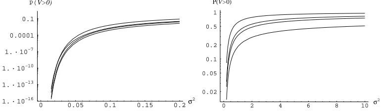
In addition to the bounds of Proposition2.9, we propose the following convenient approximation: P(V >0)≈2 P(Xt >c) =2Φσ(c). (2.15) A heuristic motivation goes as follows. P(Xt>c)is the probability that the buffer is non-empty and going up. (2.15) guesses that during busy periods, the buffer goes down roughly as often as it goes down.

A comparison of the lower and upper bounds and two heuristic approximations is presented in Figure2.1. Note that they all are based only on the one-dimensional marginal distribution of X .

0 0.05 0.1 0.15 0.2σ

2

1. · 10-16 1. · 10-13 1. · 10-10 1. · 10-7 0.0001 0.1

P(V>0)

0 2 4 6 8 10 σ

2

0.02 0.05 0.1 0.2 0.5 1 P(V>0)

Figure 2.1: A comparison of the bounds and approximations for P(V >0). From top: (2.8), upper bound in (2.11), (2.15), and lower bound in (2.11).

3

Examples

In this section, we present several different applications of the performance formulae. The ex-amples are mostly Gaussian counterparts of standard queuing systems. An interesting and very important question is how well the Gaussian counterpart approximates the original input process. If the input process only consists of a single stream, then the Gaussian version is certainly poor, but if the number of independent streams increases then the accuracy of the Gaussian approxima-tion improves. This aspect is worth of own study and we will only consider differences between our approximations and true Gaussian systems. The comparisons are performed with known ana-lytical results or simulations.

3.1

Gaussian counterpart of M

/

D

/

1

Work arrives in quanta of size 1 according to a Poisson process with parameterλ. Then v(t) =

Var(At) =λt, and the corresponding centered Gaussian process is a Brownian motion (in fact, this would be the case also with compound Poisson input). Then

t∗=x, 1

2kfx,t∗k

2

R=2 x

-2 -1 1 t 1

Queue length

-2 -1 1 t

1 Input rate

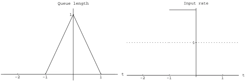
Figure 3.1: The most probable storage path in{V0≥1}and the corresponding input rate for

Brownian motion; v(t) =t. The dotted line shows the server rate c=1.

and the basic approximation happens to be exact for the Gaussian model (this fact about the maximum of a Brownian motion with negative drift is included in most textbooks). The most probable queue evolution consists of symmetric straight lines up and down (see Figure3.1).

3.2

Gaussian counterpart of nD

/

D

/

1

Work arrives in quanta of size one from n periodic sources with period d and uniformly distributed phases. We have Var(At) =n_dt(1−_dt), t∈[0,d], and a natural centered Gaussian counterpart, with time scaling by factor d, is standard Brownian bridge (repeated periodically), v(t) = [t]1(1−[t]1),

where[t]1=t mod 1. Then

t∗= x

1+2x, 1 2kfx,t∗k

2

R=2x(1+x),

and the basic approximation happens once more to be exact for the Gaussian model (see [18], p. 400). Further,Γ(s,t) = 1₂([s]1∨[t]1)(1−([s]1∧[t]1)), and the most probable input path reaching

storage level x is the periodic path fx,t∗(s) =

x+t∗ v(t∗)([−t

∗_]

1∨[s]1)(1−([−t∗]1∧[s]1)).

The periodic most probable storage path in{V0≥1}is shown in Figure3.2.

3.3

Gaussian counterpart of periodic on-off sources

-2 -1 1 t 0.2 0.4 0.6 0.8 1 Queue length

-2 -1 1 t

-2 -1 1 2 3 4 Input rate

Figure 3.2: The most probable storage path in{V0≥1}and the corresponding input rate for

periodic Brownian bridge; v(t) = [t]1(1−[t]1).

Denote d=don+do f f and

˜ v(t) =

            

dondo f f d t2−

1

3dt3, t≤min{don,do f f}

−don3

3d +

d2on d t−

don2

d2t2, don≤t≤do f f

−d

3

o f f

3d +

d_{o f f}2 d t−

d_{o f f}2

d2 t2, do f f ≤t≤don

−d

2

on−dondo f f+d2o f f

3 +

d2_on+d_{o f f}2 d t−

d2_on+dondo f f+do f f2 d2 t2+

1 3dt

3_{, t≥max{d}

on,do f f}.

Then Var(At) =n ˜v([t]d), where[t]d=t mod d. This process is absolutely continuous, withγ(0) = ndon_ddo f f, giving P(V >0)≈2Φq_nd d

ondo f f

. We simplify the notation further by choosing don+

do f f =1 and v(t) =v˜([t]1). The most probable path in{V0≥1}is shown in Figure3.3.

-2 -1 1 2 t

1 Queue length

-2 -1 1 2 t

1 Input rate

Figure 3.3: The most probable storage path in{V0≥1}and the corresponding input rate for

-6 -3 3 t 1

Queue length

-6 -3 3 t

1 Input rate

-1 -0.5 0.5 t

1 Queue length

-1 -0.5 0.5 t

1 Input rate

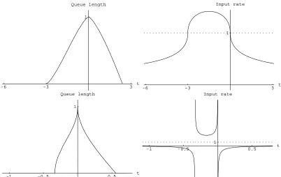
Figure 3.4: The most probable storage path in{V0≥1}and the corresponding input rate for

fractional Brownian motion; v(t) =t2H. In the upper figures H=0.75 and in the lower figures H=0.25.

3.4

Fractional Brownian motion

The input process is already a Gaussian process. Var(At) =σ2t2H, where H ∈(0,1). We have t∗= Hx

1−H, kfx,t∗k

2

R=

x2−2H

κ(H)2σ2, whereκ(H) =H

H_(1−H)(1−H)_.

The basic approximation is thus a Weibull distribution. It is not exact, but known to be a reasonably good estimate (see e.g. [13]).

Depending on the value of H, the most probable paths exhibit quite different features. When H >1/2, the process is positively correlated and the most probable path is smooth. Whereas, if H<1/2 then the input process has negative correlations causing the most probable storage path to behave oddly. In Figure3.4, these features are also clearly seen.

3.5

Gaussian counterpart of Anick-Mitra-Sondhi model

This is a fluid model [5]. Work arrives from N sources in bursts which have speed h and Exp(β) distributed lengths. After each burst the source keeps silent an Exp(λ) distributed period. The input process variance is

Var(At) =

2λβh2

(λ+β)3

t− 1

λ+β(1−e

−(λ+β)t₎

Simplifying the notation further with time scaling by factorλ+β, let us consider Gaussian input with variance

v(t) =t−1+e−t. (3.1)

The autocovariance of the rate process in this case is γ(t) = 1₂e−t. This comes from the strictly exponential autocorrelation of the rate process, and has the same form in some other popular models: Kosten’s model, where similar bursts as above start according to a Poisson process (case “N =∞”), and the renewal rate process with exponential renewal times [18]. On one hand this means that a Gaussian approach cannot make distinctions with respect to features where these models differ. On the other hand, it means that at a traffic aggregation level where the Gaussian approximation works well it does not matter which one of these models one chooses.

The most probable path with storage occupancy x at time 0 is

fx,t∗(s) = 

      

      

−2v(t

∗₎

v0(t∗)2(2t

∗_−1+e−t∗_{+ (1−e}−t∗_)es_{), s<−t}∗_,

−4v(t

∗₎

v0(t∗)2(s+e

−t∗/2₍

sinh(t

2)−sinh( t

2+s))), s∈[−t

∗_,0],

2v(t∗)

v0(t∗)2(1−e

−t∗_)(1−e−s_{), s>0.}

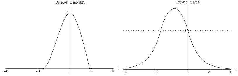
Note that this path is similar to that obtained in Shwartz and Weiss [19] as a large deviations limit of the true Anick-Mitra-Sondhi system. The corresponding most probable storage path in {V0≥1}is shown in Figure3.5.

-6 -3 2 4 t

1 Queue length

-6 -3 2 4 t

1 Input rate

Figure 3.5: The most probable storage path in{V0≥1}and the corresponding input rate for

Gaussian counterpart of Anick-Mitra-Sondhi model; v(t) =t−1+exp(−t).

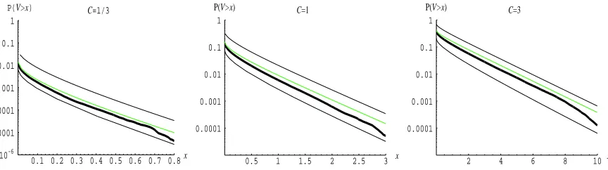
For the purpose of checking the bounds and approximations described in section2, we generated traces of the Gaussian process described above, with the variance function v(t) =C(t−1+e−t), where C is a positive parameter. These traces were fed into a simple queue with service capacity 1.

5000 10000 15000 20000 25000 30000

-100 -75 -50 -25 25 50 75

10 20 30 40 50 60

-10 -8 -6 -4 -2

1 2 3 4

-1.2 -1 -0.8 -0.6 -0.4 -0.2

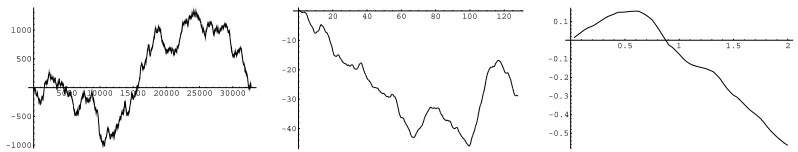
Figure 3.6: A realization of the Gaussian version of A-M-S process shown in different time scales. C=1.

C Simulation 2Φ(p2/C) upper bound lower bound

1

3 0.012 0.014 0.018 0.008

1 0.138 0.157 0.195 0.087

3 0.377 0.414 0.489 0.246

Table 3.1: Idle probabilities from simulations and the corresponding approximations.

First we consider idle probabilities. According to (2.15), we have P(V0>0)≈2P(X0>1)

=2Φ(1/pγ(0)), whereas (2.11) gives lower and upper bounds. The probabilities observed in the simulations and the corresponding approximations are shown in table3.1.

0.1 0.2 0.3 0.4 0.5 0.6 0.7 0.8x 1. · 10-6

0.00001 0.0001 0.001 0.01 0.1 1

P(V>x) _C=1/3

0.5 1 1.5 2 2.5 3 x 0.0001

0.001 0.01 0.1 1

P(V>x) _C=1

2 4 6 8 10 x

0.0001 0.001 0.01 0.1 1

P(V>x) _C=3

Figure 3.7: Gaussian counterpart of A-M-S process. P(V >x)calculated from the simulations (thick lines), the basic lower bounds (lowest lines), the basic approximations (topmost lines) and its rescaled versions (light lines).

3.6

Poisson-Pareto burst process

The term “Poisson burst process” was used in [18] for a traffic model where i.i.d. bursts with rate h start according to a Poisson process with parameterλ. Then

v(t) =λh2 Z t 0 du Z u 0 dv Z ∞ v

ds P(U>s),

where U is the generic burst length random variable. Using this family of variance functions may be the simplest way to define absolutely continuous Gaussian processes with long range dependence: just let U have a Pareto distribution with infinite variance: P(U>x) = (1/x)β∧1,

β∈(−2,−1). Let us consider the Gaussian counterpart of such a process. The variance is given by

v(t) =C

   1 2− 1 2β+2

t2−1₆t3, t<1

1 3−

1 2β+2+

1 2−

1 β+1+

1

(β+1)(β+2)

(t−1)−_(β+1)(tβ_β+₊3−₂₎₍1_β+3), t≥1,

where C>0. As in the previous examples, we can calculate the most probable path and the corresponding most probable queue evolution (see Figure3.8).

-9 -6 -3 3 6 t

1 Queue length

-9 -6 -3 3 6 t

1 Input rate

Figure 3.8: The most probable storage path in{V0≥1}and the corresponding input rate for

the Gaussian counterpart of Poisson burst model; C=1,β=−3/2.

5000 1000015000200002500030000

-1000 -500 500 1000

20 40 60 80 100 120

-40 -30 -20 -10

0.5 1 1.5 2

-0.5 -0.4 -0.3 -0.2 -0.1 0.1

Figure 3.9: A realization of the Gaussian version of the Poisson burst process with Pareto distributed bursts shown in different time scales. C=1,β=−3/2.

approaches zero (see Figure 3.9). The latter means that the idle probability should be approxi-mately 2Φ(

q

2

3C). The idle probabilities observed during the simulations and the corresponding

approximations are shown in table3.2. C Simulation 2Φ

q

2 3C

upper bound lower bound

1

6 0.039 0.046 0.058 0.024

1 0.385 0.414 0.488 0.246

6 0.717 0.739 0.811 0.499

Table 3.2: Idle probabilities from simulations and the corresponding approximations.

0.5 1 1.5 2 2.5 3 3.5 4 x 0.0001

0.001 0.01 0.1 1

P(V>x) _C=1/6

10 20 30 40 50 x 0.0001

0.001 0.01 0.1 1

P(V>x) _C=1

20 40 60 80 100x 0.01

0.02 0.05 0.1 0.2 0.5 1

P(V>x) _C=6

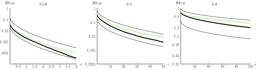
Figure 3.10: Gaussian counterpart of Poisson burst process. P(V >x)calculated from the sim-ulations (thick lines), the basic lower bounds (lowest lines), the basic approximations (topmost lines) and its rescaled versions (light lines).

The queue length distributions and their basic approximations are shown in Figure 3.10. In this case even the shifted basic approximation overestimates the tail. This is in accordance with the known, accurate asymptotics of the fBm queue (see, eg, [14,13]).

3.7

Multiplexing heterogeneous streams

All the previous examples considered homogeneous traffic. The true benefit of the proposed method is seen when we multiplex Gaussian streams with different variances. For example, it is almost impossible to handle superposition of periodic on-off sources if the periods are different. Using Gaussian approximation, the problem simplifies to calculation of the most probable storage path. The only difficulty here is to find the minimum of the function g(xv)(t) = (t+x)2/v(t), after that everything is straightforward.

2 4 6 8 10 t 6.5

7 7.5 8 8.5 9 (1+t)2_/v(t)

Figure 3.11: Minimizing g(₁v)(t); v(t) =1₂t3/2₊1

2[t]1(1−[t]1).

-4 -2 2 t

1 Queue length

-4 -2 2 t

1 Input rate

-2 -1 1 2 t

1 Queue length

-2 -1 1 2 t

1 Input rate

Figure 3.12: The most probable storage path in{V0≥1}and the corresponding input rate for

0 2 4 6 8 10 x 0.0001

0.001 0.01 0.1 1 P(V>x)

Figure 3.13: The basic approximations for P{V0≥x}. Solid line: v(t) =1₂t3/2+1₂[t]1(1−[t]1).

Dashed line: v(t) =1₂t3/2+ [t]1(1−[t]1).

The most probable storage path is strongly dependent on the ratio between coefficients c1 and

c2. If the fractional Brownian motion dominates, then the queue evolution is non-periodic, but if

the role of Brownian bridge is strong enough, then a kind of periodic behavior is observed (see Figure3.12). On the other hand, with large x, probabilities P{V>x}are determined mostly by the fractional Brownian motion, because the periodic traffic effects only on small resolutions. This is also seen in Figure3.13.

4

Conclusions

Gaussian traffic models appear to be realistic in some situations already and are likely to become more so as traffic is aggregated to higher and higher levels. In this paper, very simple and reason-ably accurate, explicit performance formulae applicable to a very wide class of Gaussian traffics have been studied. Surplus value is obtained through an immediate identification of the most probable paths to achieve a certain buffer level. The paths are built out of the covariance function of the input process. In particular, the straightforward applicability to the superpositions of very different processes offers wide possibilities of utilization in real applications.

There are a number of possible further developments from the work presented here, including refinement of the approximations, exploration of the implications for network dimensioning and planning, and extensions to more complicated systems like priority queues.

References

[2] R. Addie, P. Mannersalo, and I. Norros. Permormance formulae for queues with gaussian input. In P. Keys and D. Smith, editors, Teletraffic engineering in a competitive world (Pro-ceedings of ITC-16), volume 3b, pages 1169–1178. Elsevier, 1999.

[3] R. G. Addie. On weak convergence of long-range-dependent traffic processes. In journal of statistical planning and inference, volume 80, pages 155–171, 1999.

[4] R.J. Adler. An Introduction to Continuity, Extrema, and Related Topics for General Gaus-sian Processes, volume 12 of Lecture Notes-Monograph Series. Institute of Mathematical Statistics, 1990.

[5] D. Anick, D. Mitra, and M.M. Sondhi. Stochastic theory of a data handling system with multiple resources. Bell Syst. Tech. J., 61(8):1871–1894, 1982.

[6] R. Azencott. Ecole d’Eté de Probabiltés de Saint-Flour VII-1978, chapter Grandes devia-tions et applicadevia-tions, pages 1–176. Number 774 in Lecture notes in Mathematics. Springer, Berlin, 1980.

[7] R. R. Bahadur and S. L: Zabell. Large deviations of the sample mean in general vector spaces. Ann. Prob., 7(4):587–621, 1979.

[8] J. Choe and N. Shroff. A central-limit-theorem-based approach for analyzing queue behavior in high-speed networks. IEEE/Transactions on Networking, 6(5), 1998.

[9] J.-D. Deuschel and D.W. Stroock. Large Deviations. Academic Press, 1989.

[10] K. Kobayashi and Y. Takahashi. The tail probability of a Gaussian fluid queue under finite measurement of input process. In Proceedings of the International Conference on the Perfor-mance and Management of Complex Communication Networks (PMCCN’97), pages 57–71, Tsukuba, Japan, 1997.

[11] W.E. Leland, M. S. Taqqu, W. Willinger, and D.V. Wilson. On the self-similar nature of ethernet traffic (extended version). IEEE/ACM Transactions on Networking, 2:1–15, 1994. [12] J. Lévy Véhel and R. Riedi. Fractional Brownian motion and data traffic modeling: The

other end of the spectrum. In J. Lévy Véhel, E. Lutton, and C. Tricot, editors, Fractals in Engineering. Springer, 1997.

[13] L. Massoulie and A. Simonian. Large buffer asymptotics for the queue with FBM input. J. Appl. Prob., 36(3), 1999.

[14] O. Narayan. Exact asymptotic queue length distribution for fractional Brownian traffic. Advances in Performance Analysis, 1(1), 1998.

[15] I. Norros. A storage model with self-similar input. Queueing Systems – Theory and Appli-cations, 16:387–396, 1994.

[17] I. Norros, P. Mannersalo, and J.L. Wang. Simulation of fractional Brownian motion with con-ditionalized random midpoint displacement. Advances in Performance Analysis, 2(1):77– 101, 1999.

[18] J. Roberts, U. Mocci, and J. Virtamo. Broadband Network Teletraffic, Final Report of Action COST 242. Springer, 1996.