Investigate the use of thermal protection for underground cables in Ergon Engery's electricity network

University of Southern Queensland

Faculty of Engineering and Surveying

Investigate the Use of Thermal Protection

for Underground Cables in

Ergon Energy’s Electricity Network

A dissertation submitted by

Cosmas Gianoulis

in fulfillment of the requirements of

Course ENG4111/ENG4112 Project

towards the degree of

Bachelor of Engineering (Electrical and Electronic)

Abstract

To transmit power through an electricity transmission or distribution network is by either overhead power lines or power cables. Overhead lines are the initial and usual option as cost can be greatly reduced. Cables are more reliable as they are less impacted by weather and other environmental influences than overhead lines. They also take up less space than the alternative option.

The continued growth of consumer electricity use in Queensland, has led electricity service providers in subjecting a substantial amount of existing assets to a high utilisation ratio, even into overload to cope with the demand. Until system augmentation and further capital works are implemented to introduce greater capacity to their network, technical and engineering staffs are tasked to manipulate this network while attempting to maintaining electricity supply and reducing risk to safety and plant.

University of Southern Queensland

Faculty of Engineering and Surveying

ENG4111 & ENG4112 Research Project

Limitations of Use

The Council of the University of Southern Queensland, its Faculty of Engineering and Surveying, and the staff of the University of Southern Queensland, do not accept any responsibility for the truth, accuracy or completeness of material contained within or associated with this dissertation.

Persons using all or any part of this material do so at their own risk, and not at the risk of the Council of the University of Southern Queensland, its Faculty of Engineering and Surveying or the staff of the University of Southern Queensland.

This dissertation reports an educational exercise and has no purpose or validity beyond this exercise. The sole purpose of the course pair entitled "Research Project" is to contribute to the overall education within the student’s chosen degree program. This document, the associated hardware, software, drawings, and other material set out in the associated appendices should not be used for any other purpose: if they are so used, it is entirely at the risk of the user.

Professor R Smith Dean

Certification

I certify that the ideas, designs and experimental work, results, analyses and conclusions set out in this dissertation are entirely my own effort, except where otherwise indicated and acknowledged.

I further certify that the work is original and has not been previously submitted for assessment in any other course or institution, except where specifically stated.

Cosmas Gianoulis

Student Number: 0012909456

_________________________________ Signature _________________________________

Acknowledgements

This research was carried out under the principal supervision of Dr. Tony Ahfock, of the Faculty of Engineering and Surveying, University of Southern Queensland.

I would like to acknowledge and thank the following people for their support, guidance and assistance:

Mr. Graham Campbell – Ergon Energy Corporation

I would also like to thank my wife Maria, and my children Panayioti, Klearetti, Thomas and Kosta for their understanding and support especially in the final stages of this project.

Cosmas GIANOULIS

University of Southern Queensland

Glossary

AC: Alternating Current.

Ampacity: A term given for the current capacity of a cable.

DC: Direct Current.

DTS: Distributed Temperature Sensing, a method where a fibre optic cable is used to measure temperature along a length of cable continuously.

DNSP: Is a distribution network service provider like Ergon Energy Corporation or Energex Corporation who manage the supply of electricity to customers. They are also referred to as Electricity Entities or Electricity Service Provider.

EMF: Electrical and Magnetic Fields. It has also been used for an abbreviation for electro-magnetic force.

High voltage: relates to voltages greater than 1000 Volts.

HV: see High Voltage.

ICNIRP: International Commission on Non-Ionizing Radiation Protection.

IEC: International Electrotechnical Commission.

IEEE: The Institute of Electrical and Electronic Engineers.

kA: kiloampere = 1000 amperes.

kV: kilovolt = 1000 volts.

MW: Megawatt = 1000000 watts.

PLYS: Paper Lead Alloy Sheathed.

SCADA: System Control and Data Acquisition. An electronic system used to monitor and control elements of a process or network.

Thermal capacitiance: the material’s ability to store heat.

TNSP: Is a transmission network service provider like Powerlink Queensland Corporation who manage the supply of electricity at high voltage to DNSP’s

Symbology

A cross-sectional area of the armour mm²

B1 ω

(

)

B2 ωH₂ Ω/m

C capacitance per core F/m

* e

D external diameter of cable m

Di diameter over insulation mm

Ds external diameter of metal sheath mm

Doc the diameter of the imaginary coaxial cylinder which just touches

the crests of a corrugated sheath

mm

Dit the diameter of the imaginary cylinder which just touches the

inside surface of the troughs of a corrugated sheath

mm

H intensity of solar radiation W/m²

H magnetizing force ampere

turns/m

Hs inductance of sheath H/m

⎪ ⎭ ⎪ ⎬ ⎫

3 2 1

H H H

components of inductance due to the steel wires (see 2.4.2) H/m

R alternating current resistance of conductor at its maximum operating temperature

Ω/m

RA a.c. resistance of armour Ω/m

Re equivalent a.c. resistance of sheath and armour in parallel Ω/m

Rs a.c. resistance of sheath Ω/m

R' d.c. resistance of conductor at maximum operating temperature Ω/m Ro d.c. resistance of conductor at 20 °C Ω/m

T1 thermal resistance per core between conductor and sheath K.m/W

T2 thermal resistance between sheath and armour K.m/W

T3 thermal resistance of external serving K.m/W

T4 thermal resistance of surrounding medium (ratio of cable surface

temperature rise above ambient to the losses per unit length)

K.m/W

* 4

T external thermal resistance in free air, adjusted for solar radiation K.m/W

Uo voltage between conductor and screen or sheath V

Wa losses in armour per unit length W/m

Wc losses in conductor per unit length W/m

Wd dielectric losses per unit length per phase W/m

Ws losses dissipated in sheath per unit length W/m

W(s+A) total losses in sheath and armour per unit length W/m

X reactance of sheath (two-core cables and three-core cables in trefoil)

Ω/m

Xm mutual reactance between the sheath of one cable and the

conductors of the other two when cables are in flat information

Ω/m

a shortest minor length in a cross-bonded electrical section having unequal minor lengths

c distance between the axes of conductors and the axis of the cable for three-core cables (=0.55r1 + 0.29t for sector-shaped

conductors)

mm

d mean diameter of sheath or screen mm

d' mean diameter of sheath and reinforcement mm

d2 mean diameter of reinforcement mm

dA mean diameter of armour mm

dc external diameter of conductor mm

d'c external diameter of equivalent round solid conductor having the

same central duct as a hollow conductor

mm

dd internal diameter of pipe mm

df diameter of a steel wire mm

di internal diameter of hollow conductor mm

dM major diameter of screen or sheath of an oval conductor mm

dm minor diameter of screen or sheath of an oval conductor mm

dx diameter of an equivalent circular conductor having the same

cross-sectional area and degree of compactness as the shaped one

mm

f system frequency Hz

reinforcement (see 2.4.2.4)

kp factor used in calculating xp (proximity effect)

ks factor used in calculating xs (skin effect)

l length of a cable section (general symbol) m ln natural logarithm (logarithm to base e)

m ₁₀−7

s

R

ω

n number of conductors in a cable nn number of wires in layer n of a cable

p length of lay of a steel wire along a cable

r1 circumscribing radius of two-or three-sector shaped conductors mm

s axial separation of conductors mm

s1 axial separation of two adjacent cables in a horizontal group of

three, not touching

mm

s2 axial separation of cables mm

t insulation thickness between conductors mm

t3 thickness of the serving mm

ts thickness of the sheath mm

v ratio of the thermal resistivities of dry and moist soils

(

)

xp argument of a Bessel function used to calculate proximity effect

yp proximity effect factor

ys skin effect factor

α20 temperature coefficient of electrical resistivity at 20 °C, per kelvin I/K β angle between axis of armour wires and axis of cable

γ angular time delay

δ equivalent thickness of armour or reinforcement mm tan δ loss factor of insulation

ε relative permittivity of insulation

θ maximum operating temperature of conductor °C

θa ambient temperature °C

θx critical temperature of soil; this is the temperature of the boundary

between dry and moist zones

°C

Δθ permissible temperature rise of conductor above ambient temperature

K

Δθx critical temperature rise of soil; this is the temperature rise of the

boundary between dry and moist zones above the ambient temperature of the soil

K

λ1λ2 ratio of the total losses in metallic sheaths and armour respectively

to the total conductor losses (or losses in one sheath or armour to the losses in one conductor)

' 1

λ ratio of the losses in one sheath caused by circulating currents in the sheath to the losses in one conductor

'' 1

' 1m

λ loss factor for the middle cable

' 11

λ loss factor for the outer cable with the greater losses loss factor for the outer cable with the greater losses

' 12

λ loss factor for the outer cable with the greater losses loss factor for the outer cable with the least losses

μ relative magnetic permeability of armour material μe longitudinal relative permeability

μt transverse relative permeability

ρ conductor resistivity at 20 °C Ω.m

ρd thermal resistivity of dry soil K.m/W

ρw thermal resistivity of moist soil K.m/W

ρs sheath resistivity at 20 °C Ω.m

Table of Contents

Abstract

i

Limitations of Use ii

Certification

iii

Acknowledgements iv

Glossary

v

Symbology

vii

List of Figures xvi

List of Tables xviii

List of Appendices xix

Chapter 1 -

Introduction

1

1.1. Background...1

1.2. Project Objectives ...2

1.3. Impact to Ergon Energy...3

Chapter 2 -

Literature Review

5

2.2. Power Cable Standards ...6

2.2.1. Australian Standards ...6

2.2.2. International Electrotechnical Commission Standards ...6

2.2.3. Ergon Energy Standards...7

2.3.1. Heat Transfer...8

2.3.2. Conductor Losses ...10

2.3.3. Dielectric Losses ...12

2.3.4. Sheath and Armour Losses...14

2.4. Thermal Analogue Model Method...17

2.4.1. Thermal Resistance ...17

2.4.2. Thermal Capacitance...19

2.4.3. Van Wormer Coefficient...20

2.5. Numerical Model Methods ...21

2.5.1. Finite Element Method...22

2.6. Commercial Software Packages ...28

2.7. Distributed Temperature Sensing ...28

2.8. Protection Relays Currently in Use...31

Chapter 3 -

Methodology 33

3.1.1. Technical Research ...33

3.1.2. Cable Site Selection ...33

3.2. Data Gathering...33

3.2.1. Distribution Feeder Cables Temperatures...34

3.2.2. Distribution Feeder Daily Load Curves ...34

3.3. Model Development...35

3.3.1. Thermal Analogue Model ...35

3.3.2. Steady State Conditions ...35

3.3.3. Variable and Emergency Load Conditions ...38

3.3.3.1. Short Term Transients ...39

3.3.3.2. Long Term Transients...41

Chapter 4 -

Results and Data Analysis 43

4.2. Comparison with Commercial Packages ...46

Chapter 5 -

Conclusion 47

List of Figures

Figure 1.1 - Three core PLYS cable ...3

Figure 1.2 - Single Core XLPE Cable ...4

Figure 2.1 - Underground cable heat conduction...9

Figure 2.2 - Effects of skin and proximity phenomena ...10

Figure 2.3 - Representation of cable insulation ...13

Figure 2.4 - Standard cable layout formation ...16

Figure 2.5 - Temperature distribution for a composite cylindrical wall ...18

Figure 2.6 - Temperature distribution with a cable...20

Figure 2.7 - Short term transient representation ...20

Figure 2.8 - Long term transient representation...21

Figure 2.9 – A typical thermal network model of a cable ...21

Figure 2.10 - Triangular or quadrilateral elements ...24

Figure 2.11 – Quadratic-triangular element...24

Figure 2.12 - Using different element sizes...26

Figure 2.13 - The time step, the load curve and the time elapsed...27

Figure 2.14 - Optical Time Domain Reflectometry...29

Figure 2.15 - Backscatter spectrum (Brown, 2003)...30

Figure 2.16 - Fibre optic incorporated with the cable (Peck et al. 2000) ...30

Figure 2.17 - Fibre optic laid beside cables (Peck et al., 2000)...31

Figure 3.2 - Equivalent thermal network with two loops ...39

Figure 3.3 - Network for short duration...39

Figure 3.4 - Network for long duration...41

Figure C.1 - Temperature against Load - Real Data...61

Figure C.2 - Location of RTDs ...63

Figure D.3 - SEL Feeder Management Relay...64

List of Tables

Table 4.1 - Steady State loading ...44

Table 4.2 - Effect of depth to ampacity ...44

Table 4.3 - Soil temperature effect ...45

Table 4.4 - Soil resistance effects ...45

Table 5.1 - Maximum continuous conductor temperatures for PLYS up to 36kV...55

Table 5.2 - Maximum conductor temperature for the specified insulation...55

Table 5.3 - Skin and proximity effects...56

Table 5.4 - ε and tan δ values for insulation of power cables...57

Table 5.5 - Phase to ground voltage where dielectric loss should be calculated...57

Table 5.6 - Australian standard conditions to use...58

Table 5.7 - Ergon Energy's Standard Cable List...58

Table 5.8 - Manufacturer's cable data and installation details...59

Table 5.9 - Rating factors for soil temperature variation...59

Table 5.10 - Rating factors for cable depth...60

Table 5.11 - Soil resistivity derating factors...60

List of Appendices

Appendix A - Project Specification 54

Appendix B -

Standard Cable Data 55

Appendix C - GA11 Feeder Data 59

Appendix D - Protection Relay Information 64

Chapter 1 - Introduction

1.1. Background

The continued growth of consumer electricity use in Queensland, has led electricity service providers in subjecting a substantial amount of existing assets to a high utilisation ratio, even into overload to cope with the demand. This demand increase is due varying factors including increasing population, mineral resource boom (includes mines and smelters) and the affordability of white goods, the list is not exhaustive but indicative.

In the last decade, electricity consumption in Queensland has increased 53 percent to an annual usage of 8200 MW. This consumption rates Queensland as the second highest electricity user in Australia (Queensland Department of Energy 2006). The electricity network in the state composes of three distinct tiers, generation providers, transmission network services provider (TNSP) and distribution network service providers (DNSP).

investigating the management of power cables and ensuring that they can be utilised to their fullest without degradation or destruction of the cable.

1.2. Project

Objectives

It is proposed that this project fulfil the following aims;

1. Research background information on the theory of heating of cables, the issues and the effects. Research information on the current Australian and Ergon Energy’s Standards to the thermal rating of cables that are being used and the effect of the varying methods of enclosures for cables.

2. Collate the feeder cable temperatures that are being monitored at an Ergon Substation and the type of enclosures i.e. the soil backfill, type of cable and its properties also the ambient and ground temperatures.

3. Compare the data collected in (2) and compare the results with existing software packages in use in Ergon.

4. Research and understand the capabilities of the Schweitzer SEL Protection Relays for possible thermal protection implementation.

5. Develop a mathematical model to predict the temperature curve to suit the varying parameters such as the type of cable, the soil properties, the load curve for the cable and other environmental factors such as air and ground

temperatures to use in the protection relay.

If time permits

6. If in (5) it is not possible for the relay to employ the thermal protection, then review the possibility of the SCADA RTUs to facilitate the function.

8. Evaluate the possibility of extending the use of the model in (5) above to other protection relays in Ergon’s network.

1.3.

Impact to Ergon Energy

As the network grows some of the existing equipment are then subjected to higher loads and greater fault levels. In the Ergon network, the fault levels on the lower high voltages (11kV to 33kV) vary from 4kA to as high as 34kA.

Ergon has numerous types of high voltage cables in use around Queensland, but the most common types are XLPE and PLYS in single and multi-cored. The XLPE type of set sizes are now the common standard for new and replacement cables in the network. Figure 1.1 and Figure 1.2 displays a typical make up of an PLYS and XLPE cables.

Textile serving

Steel armour

Lead sheath

Paper or jute worming

Belt insulation

Oil impregnated paper

conductor

Figure 1.2 - Single Core XLPE Cable

(OLEX - Cables to IEC and Aust. Standards for Medium and High Voltage, P. 5)

In the past the ratings and capabilities of the transporting medium (lines and cables) have traditional been based on the manufacturers’ datasheets. The move to the use of dynamic thermal ratings has emerged to allow the electricity asset owners to manage and expose their plant to a higher utilisation factor.

Dynamic thermal ratings are based on the environment the equipment is situated in and its exposure to the elements such as wind, moisture and temperature. The calculation of the ratings of cables is more difficult than aerial lines due to the thermal dissipation being hindered by the type of enclosure albeit direct buried, in conduits or ducts and the proximity of other heat dissipating equipment (other cables).

As with any conductor excessive heating may cause irreparable damage and the move to using thermal protection is one path to mitigate the risk of plant damage and the reduction of safety to the public.

Chapter 2 - Literature Review

2.1.

Power Cable History

The introduction of power cables was inevitable with the introduction of incandescent lighting, but cables capable for the use in high voltage networks first appeared in the 1885 when the City of Vienna installed cable for its 2kV network. This cable was insulated with rubber and protected by lead armour. This initial step paved the way forward for improvement and acceptance worldwide. A brief chronological list is presented below highlighting important events in high voltage cables.

• 1890 – Ferranti developed the first oil impregnated paper cable.

• 1891 – Ferranti’s cable was installed in London for its 10kV network.

• 1917 – Oil filled cable principle developed by Emanueli.

• 1928 – Oil filled cable installed for use in the 66kV network in London.

• 1931 – Emanueli’s cable used in the 132kV network in Chicago.

• 1932 – First oil filled pipe cable used in North America, the inventor was Benett.. This lead the path for other oil filled cable constructions.

• 1964 – XLPE made a strong impact for use as a medium high voltage cable.

• 1969 – Polyethylene cable used for 225kV network in France.

• 1980 – Flexible SF6 filled high voltage cable designed for up to 362kV.

2.2.

Power Cable Standards

2.2.1. Australian Standards

Australian Standards (AS 1026-2004, AS 1429.1-2006, AS 1429.2-1998) define the mechanical composition requirements and the installation of cables. The maximum operating temperatures of the cables are also listed in these standards. These can be higher if specified by the cable supplier. These tables are listed in Appendix B -Standard Cable Data.

The AS/NZ standards do not deal with the cable ampacity. The calculation of ratings for cables is covered in the IEC standards that are dealt with next.

2.2.2. International Electrotechnical Commission Standards

As the Australian Standards does not delve into any current capacity ratings for cables, they do reference the IEC Standards 60287 and 60853 series for ratings of power cables. The 60287 series deal with the current capacity at 100 percent loading while the 60853 series cover the ratings required for cyclic and emergency use.

The IEC standards mentioned above break the ratings of cables into two voltage groups, for cables not greater than 36 kV and for those above 36 kV. These two voltage groups are separated by two categories, cyclic rating and emergency rating. Cyclic rating is based on a daily load curve where the load varies over a 24-hour period and each day is relatively the same. In emergency ratings, if the period is for greater than one hour then the use of the cyclic rating should be used else it is based on the load being between ten minutes and one hour.

temperatures and thermal resistivity of soil in various countries. This part also provides an outline of the information required from the purchaser for the selection of the appropriate type of cable. This information if given to the manufacturer will ensure that the cable will be suitable for the type of operation it is required for and removes any assumptions the manufacturer must make.

Where the IEC (60287 and 60853 series) define the necessary rating algorithms but the implementation of this into real time varies with the situations presented, these include the thermal resistivity of the soil, which is largely dependant on the moisture migration or with differing soil compositions and their thermal characteristics. The makeup of power cables normally entails the use of a conductive protective sheath and IEEE Standard (575-1988) describe the methods for calculating induced voltages and methods for bonding these sheaths to ground.

2.2.3. Ergon Energy Standards

Ergon Energy via its Network Planning Criteria Version 2.03, initially select all works proposals based on using overhead constructions and then only varies this decision based on justifiable external factors. Some of the factors that may influence the use of cables are;

• Local Government conditions for subdivisions.

• Regional Business Areas as defined by individual Regions may be all undergrounded.

• Vegetation Management in environmentally sensitive areas.

• World Heritage areas.

• Cultural Heritage considerations.

• Flight paths associated with registered air strips.

• Local community expectations.

• Contribution to costs by Third-Parties.

Ergon Energy uses standard industry tabulations and supplier manuals to rate underground cables. Currently where warranted in some situations a detailed investigation may be performed to determine actual cable ratings.

2.3. Thermal

Issues

The aim of cable ratings is to maximise the permissible current flow through a cable to a given maximum operating temperature. The current flow causes the cable to heat and this in turn limits the loading capacity. Heating of cables is one of the major problems encountered with underground systems. There are generally two types of heat losses in a cable and these are current and voltage dependant losses. In this section, we will not deal with pipe-type cables, as Ergon Energy does not have any of these types in operation.

2.3.1. Heat Transfer

To calculate the current carrying capacity of cables, the rate of heat dissipation needs to be dealt with. The heat generated by the cable due to the losses (presented later in this chapter), need to be transferred away from the cable to ensure that the maximum operating temperature is not exceeded. Heat is transferred through the cable to the surrounding environment in several manners.

Cables that are installed underground, heat transfer is by conduction from the conductor to the other parts of the cable and finally to the surrounding medium. Convection and radiation or the most common found in cables exposed to air. As cables exposed to air have a higher rate of heat dissipation than those enclosed underground, the heat transfer may be expressed as per Fourier’s law. The heat flux or transfer rate can be expressed as

2 W/m 1

dx d

q θ

ρ

−

y

x

dx dy

Wy

Wx Wx+dx

Wy+dy soil

Figure 2.1 - Underground cable heat conduction

In reality, the length of the cable is far greater than its diameter and the end effects can be neglected. In Figure 2.1 above, we can apply Fourier’s Law of heat conduction Watts x S W_x ∂ ∂ − = θ ρ (2.2) where

Wx = heat transfer rate through area S in x direction (W) ρ = thermal resistivity (K· m/W)

S = surface area perpendicular to heat flow (m2₎

x ∂ ∂θ

= temperature gradient in x direction

This leads to the heat transfer across all surfaces perpendicular to x and y to be expressed as a Taylor’s series expansion and neglecting the higher order terms gives the following equations.

t c W y y x x ∂ ∂ = + ⎟⎟ ⎠ ⎞ ⎜⎜ ⎝ ⎛ ∂ ∂ ∂ ∂ + ⎟⎟ ⎠ ⎞ ⎜⎜ ⎝ ⎛ ∂ ∂ ∂

∂ θ θ

ρ θ ρ int 1 1 (2.4)

2.3.2. Conductor Losses

Current flowing through a conductor will generate heat and the amount is often referred in joules, Watts per metre (Wc or W/m) or I2R losses from the standard power calculations Wc = I2R. This heat generated in the cable has to be dissipated into the surrounding soil or air. The resistance R should be kept to a minimum to reduce this heating effect. This resistance is mainly due to two factors, skin (ys) and proximity (yp) effects which is visualised in Figure 2.2 below. In most cases the manufacturer will provide the AC and DC resistances for varying configurations but we will show the alternate method of calculations should the AC resistance not be known.

(

)

R= ' 1+ + _(2.5)

Load current

Proximity eddy current

Skin

eddy current

Figure 2.2 - Effects of skin and proximity phenomena

Skin Effects

conductors which allow for the skin effect to be negligible for cables less than 150 mm2, this is shown in the equations (2.6) and (2.7).

7 ' 2 ₌8 _⋅10−

R f

x π (2.6)

s s s k R f k x x 7 ' 2

2 _{= =}8π _⋅10−

(2.7)

The skin effect factor is obtained using the values of ks in Table B.3, which came from IEC 60287-1-1 page 63. In most cases the xs is usually lower than 2.8 and the equation presented in (2.8) applies. The standards also mention alternative standard formulae to be used for tubular or hollow stranded conductor.

For 0< x_s ≤2.8

2 4 8 . 0 192 _s s s x x y + = (2.8)

For 2.8<x_s ≤3.8

2 0563 . 0 0177 . 0 136 .

0 _{s s}

s x x

y =− − + (2.9)

For 3.8< x_s

15 11 2 2 − = s s x y (2.10) Proximity Effect

The “Proximity effect” is multiple conductors close together create mutual reactance into each other increasing the AC resistance of the cable. This is visualised as the current densities on the sides facing each are decreased and those on the opposite side are increased due to the differences in the densities of magnetic flux.

p p p k R f k x

In the majority of cases the xp≤ 2.8 and in the IEC 60287 where the configuration is a two-core or two single-core cables, the following approximation can be used.

ay

y_p =2.9 (2.12)

For three-core cables or three single-core cables,

⎟ ⎠ ⎞ ⎜ ⎝ ⎛ + + = 27 . 0 18 . 1 312 . 0 2 2 a y ay

y_p (2.13)

where s d y x x a c p p ₌ + = ₄ 4 8 . 0 192 (2.14)

dc is the diameter of conductor (mm);

s is the distance between conductor axes (mm).

For cables in flat formation, s is the spacing between adjacent phases. Where the spacing between adjacent phases is not equal, the distance will be taken ass= s1×s2 .

2.3.3. Dielectric Losses

Figure 2.3 - Representation of cable insulation

To calculate the capacitance C the introduction of the relative permittivity of the dielectric ε is required and this is usually constant for each type of material. This is a ratio of the capacitance to the capacitance of the same material and size in a vacuum C0.

0

C C =

ε _(2.15)

This leads to the standard calculation for circular insulation, F/m 10

ln 18

9

0 ⋅ −

⎟⎟ ⎠ ⎞ ⎜⎜ ⎝ ⎛ = ⋅ = c i d D C

C ε ε

(2.16)

where

Di = external diameter of the insulation in mm.

dc = diameter of the conductor including screen if any in mm.

ω ω δ C R U C R U I I i i c r 1 tan 0 0 ₌ = = (2.17)

The equation for the dielectric loss per unit length in each phase is,

W/m tan

2 0 2

0 _{ωCU δ}

R U W

i

d = = (2.18)

Using Table B.5, dielectric losses need to be calculated for those insulation materials where the phase voltage is greater than or equal to the values given in the table. If the voltages are less than those indicated, then the dielectric loss may be ignored.

2.3.4. Sheath and Armour Losses

As the purpose of conductors is to carry current, this alternating current induces e.m.f.s in the cables metallic sheath that further reduces the current carrying ability. These losses are current dependant and under certain circumstances, large currents can flow in these coverings. These losses fall into two categories, circulating current ( ) and eddy current losses ( ). ' "

" 1

λ λ1

The first is only found in single core cable systems where the sheaths are bonded together at two points usually at the ends of the cables. This sheath acts as a parallel conductor to the cable and the induced current flows along the sheath and returns via the sheath of other phases or via the earth. This can be reduced by increasing the sheath resistance and the three single-phase cables of a three-phase system are brought close together. This does however introduce increased eddy currents and mutual heating of the cables.

" 1 ' 1 1 λ λ

λ = + (2.19)

The loss due to eddy currents is as mentioned previously, circulate radially by the skin effect and azimuthally by the proximity effect (Anders 1997). This reaches a maximum when the single-phase conductors of the three-phase system are situated as close together as possible. This can also be reduced by increasing the sheath resistance and the ratio of cable spacing to the sheath. In many cases, this loss is small compared to the circulating losses and can be ignored (Anders 1997).

Metallic armour incur losses the same as for the sheaths in relation to circulating ( ) and eddy currents ( ) flowing. Since armour has magnetic properties, a further loss occurs which is caused by hysteresis. Again, this is due to the amount of magnetic

' 2 λ

fields produced from its own conductor or other in close proximity. These combined magnetic fields can cause significant hysteresis losses (Wijeratna et al).

" 2 ' 2 2 λ λ

λ = + (2.20)

Those cables that have nonmagnetic armour, the usual practice is to take the combined sheath and armour resistance as a whole, and calculate the loss as sheath loss.

The IEEE Standard 575 introduces guidelines into the calculation of induction in cable sheaths and recommends various methods of sheath bonding. The most common types of bonding are single point, double or multiple points and cross bonding.

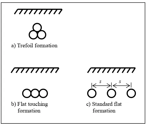
The single and multi-point bonding have some advantages and disadvantages. Since one end is not connected directly to ground, this breaks the possible circulating currents, but the open end, especially on long cables may have potentially high voltage rise on the sheaths. This can be overcome by use of sheath voltage limiters. In single point bonding for a line to ground fault, the current must return via the earth. For multi-bonding, the ground fault currents will return via the cable sheaths. Of course, the main disadvantage to these types of bonding is the reduced current carrying capacity of the cables. Cross bonding has similar properties to multi-bonding except for the almost nonexistent induction for parallel lines. Ergon Energy employs the double bonding method in its cable installations and this will be focus. Since we deal with three-phase systems the loss factors λ1 can be calculated for the two standard laying formations of trefoil (Figure 2.4 a) and flat (Figure 2.4 b & c). In both cases the =0. "

a) Trefoil formation

b) Flat touching

formation c) Standard flat formation

s s

Figure 2.4 - Standard cable layout formation

For three single-core cables in trefoil formation and bonded at both ends,

2 ' 1 1 1 ⎟ ⎠ ⎞ ⎜ ⎝ ⎛ + ⋅ = X R R R s s λ (2.21)

where X is the reactance per unit length of sheath or screen given by;

/m 2

ln 10

2 7 ⎟Ω

⎠ ⎞ ⎜ ⎝ ⎛ ⋅ ⋅ = − d s X ω

For three single-core cables in flat formation and bonded at both ends,

2 1 ' 1 1 1 ⎟⎟ ⎠ ⎞ ⎜⎜ ⎝ ⎛ + ⋅ = X R R R s s λ (2.22)

where X1 is the reactance per unit length of sheath or screen given by;

/m 2

2 ln 10

2 7 3

1 Ω ⎭ ⎬ ⎫ ⎩ ⎨ ⎧ ⎟ ⎠ ⎞ ⎜ ⎝ ⎛ ⋅ ⋅ ⋅ ⋅ = − d s

X ω (2.23)

2.4.

Thermal Analogue Model Method

2.4.1. Thermal Resistance

Materials that impede heat flow away from the cable is due to its thermal resistance. Even metallic components have a small amount of resistance but is negligible in any calculations required. An analogy between electrical resistance and thermal resistance may be associated with the driving force to a corresponding transfer rate of electricity or heat.

The formula for thermal resistance of a cylindrical layer per unit length is

1 2

ln

2 r

r T th

π ρ

= _(2.24)

For a rectangular wall

S l

T =ρ_th (2.25)

This is similar to Ohm’s Law

S l I

V V

R= 1− 2 =ρ_{el (2.26)}

Which gives way to a thermal equivalent to Ohm’s Law

tot amb 1

T T W

θ θ

θ

− =

Δ =

(2.27)

As conduction and convection resistances are in series then they may be added up to give

h r r

r r

r r

r

T A B C

4 3

4 2

3 1

2 tot

2 1 ln

2 ln 2 ln

2 π π

ρ π

ρ π

ρ

+ +

+

= _(2.28)

2.4.2. Thermal Capacitance

As mentioned previously, many cable-rating issues are time dependant. This is typical where two circuits are sharing equal load and suddenly one of the circuits switches off. The load increase on the cable in service causes a slow change in the increase in temperature distribution within the cable and the surrounding environment.

As Anders (1997, p 39) describes, “The thermal capacity of the insulation is not a linear function of the thickness of the dielectric. To improve the accuracy of the approximate solution using lumped constants, Van Wormer, in 1955, proposed a simple method of allocating the thermal capacitance between the conductor and the sheath so that the total heat stored in the insulation is represented.”

Since the thermal properties are directly involved with resistance and capacitance, correlation between electrical and thermal networks exists.

th th Q W C Q V

= Δ

= Δ

θ

: Thermal

: Electrical

(2.29)

The thermal capacitance is given by Vc

Q_th = (2.30)

(

)

Qth 22 12

4 −

=π (2.31)

where

V = Volume (m3)

c = Specific heat (J/(m3_·K)) D1 = internal diameter (m) D2 = external diameter (m)

2.4.3. Van Wormer Coefficient

As mentioned in 2.4.2, an approximate solution can be obtained by creating lumped thermal constants. Van Wormer created a ladder network representation of a cable and its surroundings for both short and long-term transients. Short term transients are accepted globally as to the duration of the transition not to be greater than ⅓ΣT ·ΣQ, which usually last anywhere between ten minutes to about one hour. These will be of interest when looking at emergency ratings.

Figure 2.6 - Temperature distribution with a cable

The distribution factor p can be calculated as

1 1 ln

2 1

2 − ⎟ ⎠ ⎞ ⎜ ⎝ ⎛ − ⎟⎟ ⎠ ⎞ ⎜⎜ ⎝ ⎛ =

Ds D d

D p

i c

i (2.32)

Figure 2.8 - Long term transient representation

Figure 2.9 – A typical thermal network model of a cable

2.5.

Numerical Model Methods

solve accurately. The iterative approach is used to calculate the ampacity of the cables. The iterative method is by specifying a certain conductor current and calculating the corresponding conductor temperature. The current is adjusted and the calculation repeated until the specified temperature is found convergent within a specified tolerance (maximum operating temperature).

In the calculations previously, separate computations are required for the internal and external parts of the cable. An assumption was made that the heat flow into the soil is proportional to the attainment factor of the transient between the conductor and the outer surface of the cable (IEC 62095). The addition of the capability of a numerical method is that in cases where the other cables are actually touching, the analytical method treated each cable separately and summated the heat flows. In finite element and difference methods, the temperature rise caused by simultaneous operation of all cables is considered. A direct solution of the heat conduction equation employing the finite element method offers such a possibility.

Each method has its issues. Some difficulties may arise when using finite element method as it does not handle well in modeling long thin objects, such as cables, in three dimensions. The finite difference method is suitable for modelling three dimensional cable problems. This method is intended for use with rectangular elements and hence is not well suited for modelling curved surfaces. The other method mentioned being the boundary elements method requires less data input and computational processes but is not suited for transient analysis.

2.5.1. Finite Element Method

The IEC standard 62095 for numerical methods deals with the finite element method. This method is used to solve partial differential equations that culminate to form the heat transfer of cables. ‘The fundamental concept of the finite element method is that temperature can be approximated by a discrete model composed of a set of continuous functions defined over a finite number of sub-domains. The piecewise continuous functions are defined using the values of temperature at a finite number of points in the region of interest’ (IEC 62095, p15).

a) A finite number of points in the solution region is identified. These points are called nodal points or nodes.

b) The value of the temperature at each node is denoted as variable which is to be determined.

c) The region of interest is divided into a finite number of sub-regions called elements. These elements are connected at common nodal points and collectively approximate the shape of the region.

d) Temperature is approximated over each element by a polynomial that is defined using nodal values of the temperature. A different polynomial is defined for each element, but the element polynomials are selected in such a way that continuity is maintained along the element boundaries. The nodal values are computed so that they provide the "best" approximation possible to the true temperature distribution. This approach results in a matrix equation whose solution vector contains coefficients of the approximating polynomials. The solution vector of the algebraic equations gives the required nodal temperatures. The answer is then known throughout the solution region.

In solutions for cable ratings, the model is usually in two dimensional plane of x and y and are generally either triangular or quadrilateral in shape. The element function becomes a plane (Figure 2.10) or a curved surface (Figure 2.11). The plane is associated with the minimum number of element nodes, which is three for the triangle and four for the quadrilateral.

Figure 2.10 - Triangular or quadrilateral elements (IEC 62095, p.23)

Figure 2.11 – Quadratic-triangular element (IEC 62095, p.23)

Size of the Region

Boundary locations is an important consideration. The objective is to select a region large enough so that the calculated values along these boundaries concur with those in the physical world. The earth’s surface is one such boundary but the bottom and sides need to be defined in such a way that the nodal temperatures all have the same value and that the temperature gradient across the boundary is equal to zero.

‘Experience plus a study of how others modelled similar infinite regions is probably the best guide. In our experience, a rectangular field 10 m wide and 5 m deep, with the cables located in the centre, gives satisfactory results in the majority of practical cases’ (IEC 62095, p 25).

The radius of the soil out to which the heat dissipates will increase with time in transient analysis. Practically it is sufficient to consider the radius that a sensible temperature rise will occur. This can calculated by

⎥ ⎥ ⎦ ⎤ ⎢

⎢ ⎣ ⎡

⎟⎟ ⎠ ⎞ ⎜⎜ ⎝ ⎛ − − =

t r Ei WI s t

r _{π δ}

ρ θ

4 4

2

, (2.33)

where θr,t is the threshold temperature value at the distance r from the cable axis. This value can be taken as 0.1 K when the number of cables is not greater than 3 and suitably smaller for a large number of cables (Anders, 1997).

Element Size

(b) (a)

Figure 2.12 - Using different element sizes

Boundary Conditions

The finite element method allows for the representations of different boundary conditions and random boundary locations, these include straight line and curved boundary representations. For current ratings, three different boundary conditions are relevant. Isothermal condition exists if the temperature is known along a section of the boundary. This temperature may be a function of the surface length. If the conditions in IEC 60287 are to be modelled then this temperature is the ambient temperature at the depth of the buried cable.

A convection boundary exists if heat is gained or lost, and should be used when large diameter cables are installed close to the ground surface. If this is the case then the user must specify the heat convection coefficient and air ambient temperature. This coefficient ranges from 2 to 25 W/m2·K for free convection and 25 to 250 W/m2·K. The third type of condition is the constant heat flux boundary condition. This is usually required when there are other heat sources in the vicinity of the cables under examination.

Representation of Cable Losses

Selection of Time Step

As computations in the finite element method require evaluation of temperatures in increments of time, the size of the time step is crucial for the accuracy of the computations.

The duration of the time step, Δτ, will depend on

a) the time constant, ΣT • ΣQ of the network (defined as the product of its total thermal resistance (between conductor and outer surface) and its total thermal capacitance (whole cable)),

b) time elapsed from the beginning of the transient, τ, and

c) the location of the time τ, with relation to the shape of the load curve being applied.

Δτ

τ

Figure 2.13 - The time step, the load curve and the time elapsed

These conditions are suggested for the selection of the time step Δτ (CIGRE, 1983),

2.6.

Commercial Software Packages

Both packages available to Ergon Energy are CYMECAP (http://www.cyme.com/software/cymcap/) and SIROLEX (http://www.olex.com/). Both of these packages use the finite element methods utilising both the Neher - McGrath and IEC 60287 methods. I have only been able to find two other package that deals specifically with power systems and both were American companies, that is USAmp (http://www.usi-power.com/Products&Services/USAmp/USAmp.html) and Ampcalc (http://www.calcware.com/index.html). This program only utilises the Neher-McGrath method, which is expected as most American ratings are based on this. I expect that there are others including a substantial amount of in-house programs that companies would have developed to assist in the ratings debate.

All of these packages use a graphical user interface that operates in a Microsoft Windows environment. As I do not have access to these programs, I could review little in regards to the actual operation of the software.

2.7.

Distributed Temperature Sensing

The emergence in the use of DTS for real time temperature monitoring of cables has introduced a more accurate method of enabling cables to be utilised to a maximum, determination of hot spots and prediction of the life span of cables. Before DTS, the measuring of real time temperatures on cables was with Thermocouples and thermisters to provide localised temperature measurement. These devices are inexpensive, and have good reliability and accuracy. They did have limitations, they only measure temperature at a single location and as a result of these discrete measurements, “hot spots” may be missed.

reflection (distance along the cable). The main backscatter from the laser pulse is in the Rayleigh Band, which is the same wavelength as the light pulse that was launched and is the strongest signal returned. The weakest of the backscatter waves are those that have been disturbed by atomic and molecular vibrations (heating).

Figure 2.14 - Optical Time Domain Reflectometry

Figure 2.15 - Backscatter spectrum (Brown, 2003)

The ‘Stokes’ band (upper band) is stable and has little temperature sensitivity. The lower band or ‘Anti-Stokes’ band has sensitivity to temperature and higher the energy in the band means greater the temperature. Accuracy within 1 degree and 1 metre is achievable with this technology.

Figure 2.16 - Fibre optic incorporated with the cable (Peck et al. 2000)

cable contracts from suppliers. The fibre optic can be included in the manufacture of the cable or laid externally with the cable.

Fibre optic cable

Figure 2.17 - Fibre optic laid beside cables (Peck et al., 2000)

2.8.

Protection Relays Currently in Use

Ergon Energy has a diverse selection of protection relays that it uses in the distribution network, and they fall into two categories, electromechanical and solid state. Since the inauguration of Ergon Energy from six Queensland regional electricity boards into one, the move for standardisation of equipment is well underway.

The type of protection relay and its requirements are revised every two years and a contract is awarded to a preferred supplier. Earlier this year the Schweitzer Company is the main supplier to Ergon for the SEL model relays (Figure D.3). The previous contractor was Alstom with the Micom series relay (Figure D.4). Should the supplier not be able to accommodate any requests of certain functionalities in the relay from Ergon, the relay may be purchased from an alternate source.

programmable logic to perform varying protection functions such as overcurrent (including directional), high impedance ground faults, under and over frequency and voltage. It can also handle synchronising checks; perform programmable auto reclosing, and detection of phase sequencing and unbalance issues. The relays of today also incorporate fault location and metering capabilities.

At the time of undertaking the project, it was thought that the SEL relay could be programmed for thermal protection. This was not the case as the only relays that have thermal functionality are the SEL 701 Monitor relays. However it was found that the Micom P14x relay includes a thermal overload feature.

The overload feature provides both an alarm and trip stage. The logic is based on the thermal element capable of being set by a single or dual time constant equation as shown below (Asltom 2004).

Single time constant:

(

)

t τ (2.35)

Dual time constant:

(

)

/ _0.6 1.05

4 .

0 1 1

I I

I I

e

e t τ t τ (2.36)

where

I is the overload current

Ip is the pre-fault steady state load

t is the time to trip

Chapter 3 - Methodology

3.1. Preliminary

Tasks

3.1.1. Technical Research

To implement any methods into a project there is a requirement to ensure that the problem at hand is understood. The main section of the research required knowledge on the effects and issues with power cables and their current rating capability. This was accomplished by the reviewing the existing Australian and IEC standards, the Ergon Network Planning and Security Criteria and other relevant written material. Most of this material was dealt with in the previous chapter. The assistance of some of our experience staff will also be sort.

3.1.2. Cable Site Selection

At the time of planning the research project, Ergon Energy decided to trial some Resistive Temperature Detectors (RTD) in the system. These were to be located at a substation where SCADA already exists and the temperature could be stored on the SCADA logging system.

The Garbutt substation, located in Townsville was an ideal choice as the soil in and around the area was said to have a high soil resistivity level. Further reasoning for choice of site, is that additional cables need to be installed for system augmentation. It also required some of the existing cable exits at the substation to be uncovered and moved during the process of works.

3.2. Data

Gathering

As this information was encompassed into the SCADA system, the ability to store the information regularly was not an issue. The retrieval process was somewhat if a different story. The temporary logging system used required special software by Wonderware called “Activefactory” to be installed on my computer. Once the software was installed, an interface connection is established and downloading of data into MS Excel spreadsheets is possible.

3.2.1. Distribution Feeder Cables Temperatures

Since all the exit cables were uncovered, it was decided that RTDs be installed on all of the exit cables. A drawing detailing the location of the detectors is shown in Figure C.2. Some issues did occur with the installation and will be reviewed latter in section 4.1.

It is important that at least a couple of cables be analysed especially with the different composition of cables. The two common types that are installed at this substation are the XLPE single-core 400 mm2 copper and the XLPE three-core (triplex) 240mm2 copper. The single core cable circuits are laid in the ground in trefoil formation (Figure 2.4a).

3.2.2. Distribution Feeder Daily Load Curves

To enable further analysis into the heating effects and the relationship of temperature to the currents flowing in the cables, the collation of feeder currents is required. This also allows to view any possible correlation of the heat dissipation relative to the time of the day, the loads etc. As this data is historically logged, it should not be any concern in the availability for use.

3.3. Model

Development

The critical section of the project is to try to establish the relationship between the cable and factors that affect the heat dissipation. These factors such as soil thermal resistance, the components of the cables, the load and the climate, need to be evaluated. Using the research found on the subject and the data available a model can be constructed. To enable this phase to fruit, certain analytical processes need to be constructed.

3.3.1. Thermal Analogue Model

After researching the issues surrounding the effects of heat and its dissipation away from the cable, it was initially decided to concentrate on one type of cable. If time permits then attempt to modify it to suit other cable types with little or no modification.

As mentioned in previously, the main concern with cables is the heat generated (normally in Watts or Joules) and the rate of dissipation from the cable. The total power loss in a cable is the algebraic sum of the individual losses that occur due to the varying components of the cable and the effect of EMF. These losses consist of the conductor loss (Wc), sheath loss (Ws) and armour loss (Wa).

(

)

= + +

= _{c s a c}

t W W W W

W (3.1)

As the sheath and armour loss are both a ratio of their losses to the loss due from the conductor, they are termed loss factors λ1 and λ2 respectively. These affect the cable

differently under two types of conditions, steady-state and transient.

3.3.2. Steady State Conditions

this model we will be looking at XLPE construction where the maximum temperature normally allowed for steady-state is 900 C (Table B.2).

Using equation (2.27) an equivalent ladder circuit can be constructed. Since the XLPE cable used in both single and three-core cable do not have a lead sheath but a screen, the loss T2 is not required.

Wc ½Wd

T1

½Wd Ws

T3 T4

Wc ½Wd

T1

½Wd Ws

T3 T4

T1 T1

3 3 3

(a)

(b)

Figure 3.1 - Ladder diagram steady-state for XLPE cables (a) Single core (b) 3 core XLPE cables

Using the above ladder network for XLPE the expression for the difference of temperature between the conductor and the surrounding medium is created.

(

)

[

]

(

)

1 1

2 1

T T n W W

T W

W_{c d}⎟ + _c + + + _d +

⎠ ⎞ ⎜

⎝

⎛ ₊

=

Δθ λ λ (3.2)

Since the lossees in the conductor are relative to the current it carries, gives the formula for calculating the steady-state current.

(

)

[

]

(

)(

)

To determine the current required for steady-state conditions, certain quantities are required for the calculation. The following steps may be required depending on the information given by the manufacturer.

1. Calculate the DC resistance R’ of the conductor at the maximum operating temperature. Normally the DC resistance R20 at 200 C is given by the

datasheet.

(

)

[

]

' _{0 20}

20 20 − + = = θ α ρ R R S R (3.4)

2. Calculate the skin and proximity factors of the conductor for use in the next step using the calculations presented in section 2.3.2.

3. Calculate the A.C. resistance using equation (2.5). 4. Calculate the dielectric losses Wd as per section 2.3.3.

5. Calculate the sheath loss factor for the screen by finding the sheath resistance and the reactance as per section 2.3.4 using double-bonding earth

arrangement in trefoil for the single cable. As the conductor is not large segmental construction the eddy currents are negligible, giving the sheath loss as the total loss factor.

6. Calculate T1 to give the insulation thermal resistance as per (3.5). The

three-core cable can be treated individually and then summated.

⎟⎟ ⎠ ⎞ ⎜⎜ ⎝ ⎛ + = c th d t T _{ln 1} 21

2π

ρ

(3.5)

7. The next calculation is for the serving / jacket outside the screen. This is the same as the formula (3.5) except it deals with the different diameters.

8. The external thermal resistance of buried cables is then calculated using the equation below to give T4 taking into account the thermal resistance of the

( )

( )

[

]

4 = _π +

ρ

(3.6)

9. Then using the current calculation (3.3) the value of current that causes the conductor temperature to reach the maximum cable operating temperature is found.

There will be slight variations to this according to the type of cable used.

3.3.3. Variable and Emergency Load Conditions

The previous section dealt with steady state but it causes some concern when trying to establish the rate of temperature rise due to a step response. In this section, we will try to create a model that will assist in dealing with transient load variation to assist in answering the following questions;

1. Given the current operating conditions and a load increased by a given amount and sustained for a period what will be the temperature?

2. For a given time period, what is the maximum current the cable can carry so that the conductor temperature does not exceed a specified limit?

3. Based on the current operating conditions, how long can a new higher loading be applied without exceeding a specified temperature?

The first and second questions, if answered will be of assistance in the model validation due to the cyclic nature of the cable under test. The third part would assist in dealing with emergency ratings of cables and the duration the load can be sustained. This will also assist in acquiring the parameters for the protection relays as mentioned previously.

As per the previous section, the cable was expressed as a ladder network. This will still apply but it is reduced to a two-loop network.

Figure 3.2 - Equivalent thermal network with two loops

Since this is a relatively simple circuit, it has been adopted by the IEC 60853 Part 1 and 2 as the standard and recommends that it be used for calculating transient responses. There are two types of responses, short and long term. The short term usually relates to durations longer than ten minutes to around an hour (≤ ⅓T·Q for single core cables and ≤ ½ T·Q for the total of three-core cables).

3.3.3.1. Short Term Transients

Qc+p*Qi1

½T1 ½T1

(1-p*_)Q

i1 +p*Qi2

qsT3

(1-p*)Qi2 + Qs/qs +p’Qi1/qs

(1+p’)Qj qs

QA QB

TB TA

Figure 3.3 - Network for short duration

(

)

(

)

(

)

2 3 1 3 2 3 1 1 1 2 1 2 1 2 1 Q Q T q T T q Q Q T q T T Q Q T T s s B s B A A + ⎥ ⎥ ⎥ ⎥ ⎦ ⎤ ⎢ ⎢ ⎢ ⎢ ⎣ ⎡ + + = + = = = (3.9)

Once these values are established, the cable partial transient needs to be attained by shorting out the right hand terminals in Figure 3.3. The transient resonse is as follows;

(

)

(

)

M = + +

2 1 0 (3.10) B B A AT Q T

Q

N₀ = (3.11)

0 0 2 0 0 N N M M

a= + − (3.12)

0 0 2 0 0 N N M M

b= − − (3.13)

(

)

= _{A B}

A

a bT T

Q b a

T 1 1 (3.14)

(

)

The transient temperature rise of the conductor above the surface of the cable is

( )

[

(

) (

)

]

b at a

c

c t =W T 1−e− +T 1−e−

θ (3.16)

The attainment factor for the transient rise between the conductor and outside surface of the cable;

( )

(

( )

)

= θ (3.17)

For direct buried cables the influence of the ground around the cable increases with time and may be significant within the short duration. The transient rise of the outer surface of the hottest cable within a group is;

( )

( )

∑

This finally leads us to the total transient temperature rise above ambient as;

( )

( ) ( ) ( )

θ = + ⋅ (3.19)

As temperature increases so does the electrical resistance and the resistance of any other metallic parts. To take this into consideration the following correction equation is used;

( )

(

( ) ( )

( )

)

a _{θ θ}

θ θ − ∞ + = 1 (3.20)

3.3.3.2. Long Term Transients

Qc T1 pQi T3 Qs (1-p)Qi

Wc Ws

P’Qj

(

)

As per the short duration transients the formulae from (3.10) to (3.17) are identical except for (3.18) which is replaced by the one below.

( )

( )

( )

∑

Chapter 4 - Results and Data Analysis

4.1.

Data and Model Validation

As time restrictions for this research