This is a repository copy of Sample size and the multivariate kernel density likelihood ratio : how many speakers are enough?.
White Rose Research Online URL for this paper: http://eprints.whiterose.ac.uk/120640/
Version: Accepted Version Article:
Hughes, Vincent orcid.org/0000-0002-4660-979X (2017) Sample size and the multivariate kernel density likelihood ratio : how many speakers are enough? Speech Communication. pp. 15-29. ISSN 0167-6393
https://doi.org/10.1016/j.specom.2017.08.005
[email protected] https://eprints.whiterose.ac.uk/
Reuse
This article is distributed under the terms of the Creative Commons Attribution-NonCommercial-NoDerivs (CC BY-NC-ND) licence. This licence only allows you to download this work and share it with others as long as you credit the authors, but you can’t change the article in any way or use it commercially. More
information and the full terms of the licence here: https://creativecommons.org/licenses/ Takedown
If you consider content in White Rose Research Online to be in breach of UK law, please notify us by
Sample size and the multivariate kernel density likelihood ratio: how many speakers are enough?
Vincent Hughes
University of York
Department of Language and Linguistic Science
University of York
York
YO10 5DD
UK
Abstract
The likelihood ratio (LR) is now widely accepted as the appropriate framework for evaluating
expert evidence. However, an empirical issue in forensic voice comparison is the number of
speakers required to generate robust LR output and adequately test system performance. In
this study, Monte Carlo simulations were used to synthesise temporal midpoint F1, F2 and F3
values from the hesitation marker um from a set of raw data consisting of 86 male speakers of
standard southern British English. Using the multivariate kernel density LR approach, these
data were used to investigate: (1) the number of development (training) speakers required for
adequate calibration, (2) the number of test speakers needed for robust validity, and (3) the
effects of varying the number of reference speakers. The experiments were run over 20
replications to assess the effects of which, as well as how many, speakers are included in
each set. Predictably, LR output was most imprecise using small samples. Comparison across
the three experiments shows that the greatest variability in LR output was found as a function
of the number of development speakers Ð where stable LR output was only achieved with
more than 20 speakers. Thus, it is possible to achieve stable performance with small numbers
of test and reference speakers, as long as the system is adequately calibrated. Importantly,
however, LRs for individual comparisons may still be substantially affected by the inclusion
of additional speakers in each set, even when large samples are used.
Keywords
1 Introduction
In recent years it has been claimed that forensic science has undergone a paradigm shift (Saks
& Koehler 2005) in the approaches used for analysing and evaluating expert evidence. As
outlined in Morrison (2014), essential elements of this shift involve the adoption of the
data-driven, numerical likelihood ratio (LR) for estimating the strength of forensic evidence, and
the empirical estimation of the validity and reliability of the system used to compute the LR
(for a detailed overview see Robertson & Vignaux 1995, Aitken & Taroni 2004, and
Morrison 2009). While there is general agreement across the forensic sciences that the LR is
the appropriate framework for evaluating evidence, within the field of forensic speech
science there remain practical issues associated with the computation of a numerical estimate
of the strength of voice evidence (French et al. 2010, Gold & Hughes 2014, Morrison &
Enzinger 2016). In this paper, one such issue is addressed, namely that of sample size,
focussing on the number of development, test and reference speakers required to adequately
calibrate forensic voice comparison systems, evaluate their validity, and compute robust LR
output.
Forensic voice comparison and the likelihood ratio
Forensic voice comparison (FVC) involves the comparative analysis of the speech patterns in
a recording of an unknown offender (e.g. covert recording of a drugs deal) and those in a
recording of a known suspect (e.g. police interview recording). The expert analysis of the
suspect and offender samples is used to aid the trier-of-fact in determining the innocence or
guilt of the defendant. FVC accounts for the majority of work conducted by forensic speech
scientists. Worldwide many different approaches are used for the analysis of speech samples
in FVC cases, with one of the most common being combined auditory and acoustic analysis
(Gold & French 2011, Morrison et al. 2016), based on principles from linguistic and phonetic
theory. Using this approach, a wide range of features is available to the expert for analysis,
including segmental features (consonants and vowels), suprasegmental features (fundamental
frequency, intonation, rhythm), syntax, lexical choices, and even non-linguistic features such
as hesitation markers, pauses, and coughs.
Within the field of forensic speech science there is growing, in-principle acceptance that the
Meuwly 2000, Broeders 2001, Nolan 2001, Rose & Morrison 2009). The LR is an estimation
of the strength or weight of the evidence under the competing propositions of the prosecution
and defence, expressed as:
(1)
�(�|�&) �(�|�()
where � is probability, � is evidence (i.e. the observations derived from the offender sample),
| is ÔgivenÕ, �& is the prosecution proposition and �( is the defence proposition. In FVC, the
prosecution proposition is almost always that Ôthe suspect and the offender are the same
speakerÕ, while the defence proposition can be reduced to Ôthe suspect and the offender are
different speakersÕ (for more on the importance and implications of using a carefully defined,
appropriate defence proposition see Morrison et al. 2012, Morrison & Stoel 2014, Hughes &
Foulkes 2015). The LR involves two elements: similarity and typicality. The numerator of the
LR is equivalent to the similarity between the suspect and offender samples with regard to the
features analysed by the expert. The denominator is equivalent to the typicality of the
observations of the features in the offender sample relative to patterns in the relevant
population (Aitken & Taroni 2004) (i.e. what is the probability of finding the offender values
assuming they were produced by another member of the population defined by the defence
proposition?).
LR-based system testing
In FVC casework the analyst uses a system to compute a numerical LR. In this context,
system refers broadly to Òa set of procedures and databases that are used to compare two
samples, one of known origin and one of questioned origin, and produce a (LR)Ó (Morrison
2013: 174). Systems can therefore differ in many respects, such as the features analysed, the
equation used to compute the scores, the database used to represent the relevant population,
and the methods used for the calibration and combination of LRs. Prior to the computation of
a LR for a given suspect and offender (evidential) comparison, many systems may be tested
and the best one chosen on the basis of optimum validity and reliability.
of LR-like scores are computed for a set of test data where it is known, a priori, whether the
samples contain the voices of the same speaker (SS) or different speakers (DS). In the
computation of scores, typicality is estimated based on a set of reference data representative
of the relevant population. The second stage is score-to-LR mapping. This involves
computing a second series of SS and DS scores for an independent set of development (or
training) data, again using the reference data to calculate typicality. Based on the scores for
the development data, calibration coefficients are generated (see Morrison 2013) which are
then applied to the scores for the test data to convert them to LRs. Calibration is a means of
optimising system validity and is claimed to be Òessential if one wishes to interpret system
output as (LRs)Ó (Grigoras et al. 2013: 620), although the extent to which calibration is
necessary depends on how well the statistical model fits the underlying data. The calibrated
LRs can then be used to estimate the validity and reliability of the system.
Applied to a FVC case, system testing would be performed following the procedures above.
The system with the best validity and reliability would then be fixed and used to compute and
calibrate a LR for the evidential suspect and offender comparison. The validity and reliability
of the system, based on the test data, would be presented to the court along with the absolute
value of the calibrated LR.
Sample size and the LR in FVC
A significant practical issue in LR-based FVC is the number of speakers required in each of
the development, test, and reference sets to produce robust and replicable LR output. A
relatively small body of research has addressed some elements of this issue for
acoustic-phonetic FVC. This work has largely concentrated on the number of reference speakers
needed to quantify typicality.
Ishihara & Kinoshita (2008) analysed long-term fundamental frequency (parameterised using
the mean, standard deviation, kurtosis, mode and modal density) from non-contemporaneous
samples of spontaneous speech from 241 male speakers of Japanese. The speakers were
divided into two groups, and within each group 12 differently sized population samples were
created, varying from 10 to 120 speakers. This allowed for the computation of two scores for
each comparison for the same population size. Cross-validated scores were computed for all
and typicality assessed against the differently sized reference sets. Ishihara & Kinoshita
found that median SS log10 LRs (LLR) were three orders of log magnitude greater when
using 10 reference speakers compared with using all 120. The overall range of LR scores also
decreased as the amount of reference data increased, with DS pairs more sensitive to the size
of the reference sample. With 10 speakers the median DS LLR value was around -30. Using
120 reference speakers, the DS median LLR was located between -2 and -3. Equal error rate
(EER) was also found to improve as the number of speakers increased, although
Òimprovement (was) more rapid up to the population size 30Ó (2008: 1943). The same data
were also examined in Ishihara & Kinoshita (2014), but the analysis was expanded to focus
on calibrated LR output and include Cllr and different measures of precision (including
credible intervals) as a function of reference sample size. Both validity and precision were
found to improve (i.e. reduce) as sample size increased.
While Ishihara & Kinoshita (2008, 2014) focused on the effects of small numbers of
reference speakers, Rose (2012) investigated an upper limit for reference sample size at
which point LR performance stabilises. Rose (2012) used Monte Carlo simulations to
synthesise F1, F2 and F3 midpoint values for Australian English /aː/ for up to 10,000
speakers based on data from the Bernard (1970) corpus. Monte Carlo simulations involve
generating synthetic data from a distribution which is representative of the population being
modelled. Simulations are a useful tool for testing issues of sample size, particularly when
sufficiently large sets of raw data are unavailable (a detailed overview of the procedures
involved in Monte Carlo simulations is provided at 2.3). Using both normal (Lindley 1977)
and kernel density (Aitken & Lucy 2004) LR approaches, scores were computed based on
real suspect and offender case data and assessed as a function of the number of reference
speakers between five and 60. Output was compared against what Rose refers to as the true
LR which was based on all of the available data (10,000 reference speakers). The term true is
not used by Rose to mean the statically true value Ð i.e. the actual, ground truth value for the
population under perfect conditions Ð but rather the most precise estimate of that actual value
based on the maximum amount of available data.
The results of Rose (2012) are comparable with those of Ishihara & Kinoshita (2008). Based
on univariate analyses of individual formants, SS scores were generally higher in magnitude
than the true value when using fewer than 10 speakers. The overall range of LRs was also
stable scores were achieved (within two standard deviations of the true scores) by the
inclusion of 30 reference speakers. This was the case even for F2, which displayed the
greatest sensitivity to sample size. A similar pattern was found in the multivariate analysis,
with the distributions of values skewed towards stronger scores when using small samples.
Compared with the univariate analysis, the range of scores based on the multivariate data was
far more sensitive to sample size. However, RoseÕs (2012) study was based on a single SS
comparison. Therefore, it was not possible to assess the performance of a set of test data as a
function of the number of reference speakers or assess how system validity is affected by
sample size. Further, the scores were not calibrated.
Hughes, Brereton & Gold (2013) used Monte Carlo simulations to assess the point at which
LR output becomes asymptotic with very large numbers of reference speakers (up to 1000
synthetic speakers) using univariate articulation rate (AR) data as input. The magnitude of
calibrated LLRs, as well as EER and Cllr, were found to be stable with as few as 10 reference
speakers. This suggests that for AR very small samples are sufficient for estimating the
population distribution. However, as acknowledged by Hughes, Brereton & Gold (2013),
given the relative lack of speaker discriminatory power offered by AR, the extent to which
these results are transferable to other speech features is potentially limited. Hughes &
Foulkes (2014) considered the effects of reference sample size using cubic polynomial
representations of the first two formants of /uː/ (four coefficients x two formants) across
varieties of English. Consistent with Ishihara & Kinoshita (2008) and Rose (2012), scores
were found to be misleading and spread over a wider range when using smaller numbers of
reference speakers (fewer than 10). Finally, Hughes (2014) replicated the experiment in
Hughes & Foulkes (2014) using cubic polynomial representations of F1~F3 for /aɪ/ (four
coefficients x two formants). Results were generally found to be consistent with previous
studies, although more speakers were required (around 50) before calibrated LLR output
became stable.
A number of general patterns emerge from previous research into reference sample size.
Firstly, small numbers of reference speakers should generally be avoided as they provide
misrepresentative estimations of typicality and therefore produce misleadingLR output. This
is consistent with a general principle in statistics that population distributions will be
increasingly imprecise as the size of the sample decreases (and conversely, precision will
number of reference speakers required to produce asymptotic LR output will differ across
features. In particular, sensitivity to reference sample size variation has been found to be
correlated with the dimensionality of the input feature. That is, features with higher numbers
of dimensions require more speakers to adequately model the multivariate distribution of
values in the population than features with smaller numbers of dimensions. This is evidenced
by comparing the results for articulation rate (AR) (one dimension Ð least sensitive to sample
size) from Hughes, Brereton & Gold (2013), /u:/ (eight dimensions) from Hughes & Foulkes
(2014) and /aɪ/ (12 dimensions Ð most sensitive to sample size) from Hughes (2014).
Although previous research has focused primarily on the effects of reference sample size, LR
output is also necessarily affected by the size of the development and test sets. Yet, it seems
that no empirical research has been conducted to investigate this issue. This study, therefore,
expands on previous work on sample size in LR-based FVC to examine the effects of the
number of (i) development, (ii) test, and (iii) reference speakers on the magnitude of
calibrated LRs and system validity (Cllr). Using midpoint measurements of the first three
formants of the vocalic portion of the hesitation marker um, multiple replications of each
experiment were conducted to assess the imprecision in LR output with different sample sizes
and sets of speakers. This is done using data synthesised from an existing set of data from 86
male speakers via Monte Carlo simulations. The results are considered in terms of the effects
of sample size variation in each of the development, test and reference sets individually, as
well as the potential trade-offs across sets.
2 Method
2.1 Corpus and input features
Speech samples were drawn from the Dynamic Variability in Speech corpus (DyViS; Nolan
et al. 2009). DyViS was collected for the purposes of forensic phonetic research and contains
a sociolinguistically homogeneous set of 100 male speakers of standard southern British
English (SSBE; for an overview see Kerswill 2006) aged between 18 and 25. Speakers were
recorded participating in four tasks. For the purposes of the present study tasks 1 and 2
recordings were analysed. Although collected for forensic purposes, the DyViS corpus is not
entirely forensically realistic. The two tasks were recorded on the same day, but not as part of
time between sessions (see Enzinger & Morrison 2012); however, the tasks themselves
involve different speaking styles with different interlocutors and should furnish some
forensically realistic within-speaker variability. Very little work has investigated the effects
of within-speaker variability on LR-based system performance or the relative importance of
different sources of variability. Therefore, any corpus used will necessarily not reflect all of
the relevant facts of any given forensic case. Task 1 involved a mock police interview in
which the participant was questioned about a crime. Participants were presented with slides
providing information about the crime and told to avoid incriminating information. Task 2
involved a telephone conversation with a mock accomplice. For this study, the high quality
near-end recordings were analysed. Recordings were between 10 and 30 minutes in duration,
and were digitised at a sample rate of 44.1kHz and 16 bit-depth.
Midpoint F1, F2 and F3 values from the vocalic portions of the hesitation marker um
(sometimes represented orthographically as erm) were used as input data. um was chosen as it
provides multidimensional data which are typical of many segmental acoustic-phonetic
features analysed in FVC. Therefore, procedures for simulating data develop those in
Hughes, Brereton & Gold (2013), who considered only univariate data. Hesitation markers
have also been shown to have very good speaker discriminatory power, with empirical
research suggesting that they outperform lexical vowels (Foulkes et al. 2004, Hughes 2014).
The finding that hesitation markers outperform lexical vowels is, to some extent, predictable.
Since hesitations are non-linguistic, they are not constrained by the phonological system in
the same way as lexical vowels, which offers greater scope for individual variation. Further
hesitation markers are less susceptible to coarticulation as they frequently occur adjacent to
silence. For more on the speaker discriminatory power of hesitation markers using the same
data see Hughes et al. (2016a,b).
2.2 Data extraction
Existing formant data for um from DyViS were available from Hughes et al. (2016a,b).
Tokens had been manually segmented and values for F1, F2 and F3 extracted at +10% steps
across the duration of the vowel. The To formant (burg)É function in PRAAT (Boersma &
Weeink 2014) was used for formant estimation, with the tracker set to identify between 5 and
6 spectral peaks within a range of 0 to 5 kHz. The original dataset consisted of 92 speakers
of um; see Hughes et al. 2016a) with up to 20 tokens per speaker. Initially, four speakers with
fewer than 10 tokens per session were removed from the analysis. For the purposes of the
present study only the midpoint values were used. This is because of the considerably greater
degree of complexity involved in simulating highly multivariate data such as formant
dynamics compared with three midpoint values. The raw data were inspected visually and
obvious measurement errors (e.g. F1 measured as F2) corrected by hand. Where values were
missing at the +50% step (midpoint), the mean of the two adjacent values (+40% and +60%)
was used. Where erroneous values could not be resolved, the whole token was removed from
the analysis. For two speakers, this meant that there was insufficient data for analysis and so
these speakers were also removed. The resulting dataset therefore consisted of 86 speakers,
with between 10 and 20 tokens per session per speaker, although only 11 speakers had fewer
than 20 tokens per session. A more detailed overview of the processes of data extraction and
descriptive patterns of acoustic variation in the data are provided in Hughes et al. (2016a,b).
2.3 Monte Carlo simulations
Monte Carlo simulations involve generating synthetic data from a distribution representing
the true distribution of values for a given parameter within a given population. In this study,
simulations were used to generate data for synthetic speakers from the relevant population of
male, SSBE speakers aged between 18 and 25. For each synthetic speaker, data representing
tasks 1 and 2 were synthesised (see below). Since the sampling distribution represents the
entire population, any number of speakers may be generated, allowing for multiple
repetitions of the experiments in this study using independent sets of speakers. The following
sections outline the processes used to simulate data.
2.3.1 Modelling
Data for synthetic speakers were generated using the same two-step simulation procedure
described in Hughes, Brereton & Gold (2013). This approach uses the MVKD equation as a
basis for simulating values, since MVKD is used to compute scores in the experiments in this
study. In MVKD, within-speaker variation (including data from the suspect) is modelled
using a Gaussian distribution (Morrison 2011a). Therefore, individual synthetic speaker data
for each session was modelled as Gaussian distributions. The two-stage simulation involved
speaker from the distributions of means and SDs in the raw data. Individual tokens for each
synthetic speaker were then simulated from the normal distributions parameterised by these
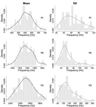
[image:12.595.131.457.148.512.2]mean and SD values.
Figure 1: Histograms of raw means (left) and SDs (right) for F1 (top), F2 (middle) and F3
(bottom) based on task 1 data for 86 speakers fitted with a kernel density
Initially, it was necessary to establish the appropriate distribution for modelling the raw
means and SDs from which to generate synthetic values. By-speaker means and SDs were
calculated for the 86 speakers for F1, F2 and F3 for each session separately. Figure 1 displays
the histograms of raw means and SDs for each formant from task 1 fitted with a kernel
density estimate. Figure 1 suggests that the normal distribution provided a relatively accurate
model of the distributions of the session means. The distributions of SDs in all three cases
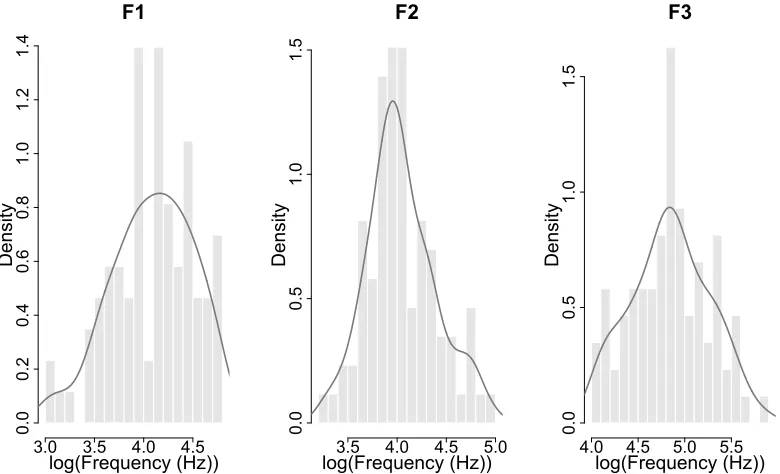
appeared positively skewed. Figure 2 displays the distributions of the natural log values of
the SDs from task 1 plotted as a histogram with estimated kernel densities. The normal
formants, the distributions of log values were relatively symmetrical, with the mean
approximately at the point of maximum density. On this basis, it was decided that synthetic
SDs would be sampled from a lognormal distribution (see 2.3.3). The lognormal distribution
is also justifiable on linguistic grounds. This is because the majority of speakers are expected
to display moderate levels of within-session variability (c. 40-100 Hz). However, while there
is inherently a floor effect in terms of potential within-session variability, there is far greater
[image:13.595.94.484.242.479.2]scope for high levels of variability for a small proportion of speakers.
Figure 2: Histograms of the natural log values of raw SDs for F1 (left), F2 (centre) and F3
(right) based on task 1 data for 86 speakers fitted with a kernel density
2.3.2 Correlations
In order to generate appropriate multisession, multivariate data it was necessary to
incorporate some within- and between-session correlations between input variables into the
simulations. Therefore, the correlation structure of the raw data was analysed prior to
conducting simulations.
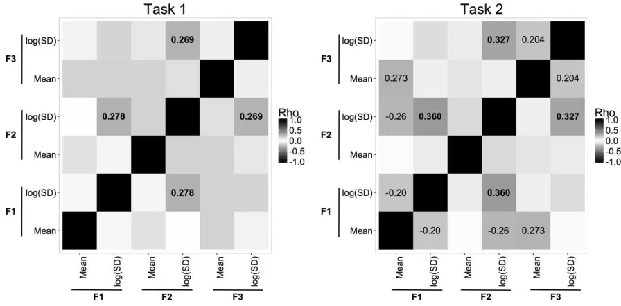
Figure 3 displays the within-session correlation matrices generated from the means and log
SDs for tasks 1 and 2 based on Pearson correlation tests. A correlation coefficient threshold
of ±0.2 was used for defining meaningful relationship, with coefficients greater than F1 log(Frequency (Hz)) D e n si ty
3.0 3.5 4.0 4.5
0 .0 0 .2 0 .4 0 .6 0 .8 1 .0 1 .2 1 .4 F2 log(Frequency (Hz)) D e n si ty
3.5 4.0 4.5 5.0
0 .0 0 .5 1 .0 1 .5 F3 log(Frequency (Hz)) D e n si ty
4.0 4.5 5.0 5.5
threshold considered for inclusion in the simulations. For task 1, two pairs of variables
generated correlations coefficients greater than threshold; F1 log SD ~ F2 log SD and F2 log
SD ~ F3 log SD. The same correlations were also found for task 2 (with larger correlation
coefficients), along with three additional pairs of variables. However, the three additional
correlations in task 2 were not included in the simulations since their absence from task 1
provides evidence that the correlations are not robustly found across sessions in the
[image:14.595.73.521.237.458.2]population at large.
Figure 3: Pearson correlation matrices for within-session correlations between F1, F2, and F3
means and log SDs for task 1(left) and task 2 (right) data (correlation coefficients of greater
than ±0.2 are marked, and correlations shared across both tasks are in bold)
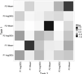
Figure 4 displays the Pearson correlation matrix for between-session correlations. Again, a
correlation coefficient of ±0.2 was used as threshold. Figure 4 reveals a complex
between-session correlation structure, with multiple variables related to each other to different extents
and in different directions. In order to simplify the simulations in this study, only the
strongest, pairwise correlations were considered. Therefore, given the size of their correlation
coefficients, the relationships between F1, F2, and F3 means were included, along with the
relationships between F1 log SDs and F2 log SDs. Although this approach captures some of
the important correlation structure in the raw data whilst also maintaining relative simplicity
in the simulation procedures, it also overestimates within-speaker variability across sessions.
correlations are assumed to be independent. This was expected to have the effect of reducing
the overall performance of the systems tested. Therefore, overall performance is expected to
[image:15.595.152.437.156.412.2]be worse than that reported in Hughes et al. (2016a,b).1
Figure 4: Pearson correlation matrix for between-session correlations between F1, F2, and F3
means and log SDs
2.3.3 Monte Carlo simulations
On the basis of 2.3.2, simulations were conducted by firstly generating independent mean F1,
F2, and F3 values from the raw task 1 data. These values represented the mean for each
formant for the synthetic task 1 data for each synthetic speaker. Having established that the
means for a single session are normally distributed in 2.3.1, the procedures outlined in
Hughes, Brereton & Gold (2013) for sampling from the normal distribution were followed to
create synthetic speaker means. The synthetic, task 1 F1 SD was also generated
1
The experiments in this study were also conducted using simulations based on contemporaneous recordings (but see Enzinger & Morrison, 2012) which assumed independence across the means and SDs of the individual formants (Hughes, 2014). The patterns were broadly the same as those reported in section 3 here, in terms of the effects of sample size, but the strength of evidence was considerably greater and the validity considerably better. This was because the evidence from each formant was statistically independent (essentially doubling of evidence where the underlying data are actually highly correlated; see Rose, Lucy & Osanai, 2004).
independently. However, the lognormal nature of the SDs for a single session (see 2.3.1) also
needed to be included in the simulations. The procedures for this are broadly the same as
those used for the normally distributed means, although the probability density function
(PDF) is defined differently for lognormal data.
The SD of F1 is denoted by �, where �∗ is the F1 SD for an individual speaker. The raw �∗
values from all 86 speakersÕ task 1 data were transformed using the natural logarithm (��),
and the mean (�) and SD (�) of the logged values calculated. These properties of the
distribution of logged values were used to define the lognormal PDF:
(2)
1
�� 2� �
4(56 748) 9
:;9
from Patel & Read (1982: 24)
Based on this, the lognormal distribution was normalised by applying the transformation:
(3)
� = (�� � − �7) 2�7
This conversion transforms linguistically meaningful values (in the �-space) to normalised �
-space values, such that the area under the normalised distribution is equal to one. Having
defined � for lognormal data, the cumulative distribution function (CDF) of the lognormal
PDF can be calculated as:
(4)
� �, 0,1 2 Β
4Χ
�� = ��� � =1 + ��� (�) 2
where:
��� = 2
� �
4Κ9�� Β
Μ
With explicit knowledge of the inverse CDF, synthetic zi values were generated using a
random variable Zi∈ [0, 1] and then converted back to the y-space by applying the
transformation:
(5)
� = �� � − �7 2�7 ,
� 2 �7 = �� � − �7
� 2 �7+ �7 = �� �
∴ � = � Β : ;ΡΣ 8Ρ
The synthetic task 1 F1 SD for each synthetic speaker (�∗) was then used to generate a task 1
F2 SD (�∗) value. Synthetic F2 SD values were sampled from a normal distribution, in the
same way as Hughes, Brereton & Gold (2013), where the mean was defined by the linear
correlation between log(F1 SD) and log(F2 SD) (see Figure 3):
(6)
� ln(�∗) + �
The SD of the sampling distribution was the mean of the residuals around the linear trend
line. The same procedure as for the synthetic mean values was then followed to generate a
synthetic log F2 SD value. The exponential of this value was then used as the synthetic task 1
F2 SD value (�∗). The same process was used to generate synthetic task 1 F3 SDs from the
synthetic F2 SDs. These procedures, finally, produced normal distributions (parameterised
using the synthetic means and SDs) for each synthetic speaker representing their task 1 data.
Synthetic task 2 data were generated entirely using correlations. Synthetic mean F1, F2, and
F3 values for task 2 were created from the synthetic mean F1, F2, and F3 values for task 1
using the correlation in the raw data and the procedure outlined above (although without the
log conversion). In this way, the simulations captured the between-session correlations whilst
maintaining the independence of the mean values within-sessions. Synthetic task 2 SDs for
F1 and F2 were created from their synthetic counterparts from task 1, based on the
the within-session correlation in 2.3.2. This approach was considered preferable to using the
between-session correlation since the within-session correlation for task 2 was stronger. This
also introduced important within-session correlation into the synthetic task 2 data which
[image:18.595.113.484.178.465.2]would have been completely absent if using only between-session correlations.
Figure 5: Cumulative distribution functions of F1 (top), F2 (middle), and F3 (bottom) means
and SDs for tasks 1 (left) and 2 (right) based on the raw data (86 speakers; dashed line) and
an example set of 1000 synthetic speakers (solid line)
The simulation procedure generated normal distributions (i.e. means and SDs) for F1, F2, and
F3 for each synthetic speaker for both tasks 1 and 2. Tokens for synthetic speakers were then
sampled independently from these normal distributions: � ~ �(�, �). In this way, the
simulation procedure may not capture within-speaker correlations across individual tokens,
which in turn may further overestimate within-speaker variability and reduce overall system
performance. These issues with the simulations are considered in section 4. In order to
evaluate the appropriateness of the simulation procedures the distributions of means and SDs
two data sets are shown in Figure 5. There was considerable overlap between the two sets,
indicating that the simulations accurately model the distributions in the raw data.
2.4 Experiments
In this study, multiple replications of the same experiment were conducted to assess the
sensitivity of LR output to variation in the number of (1) development, (2) test, and (3)
reference speakers. For each experiment, only the number of speakers in the target set (i.e.
development, test or reference) was varied to remove confounding sources of sample size
variability. Across all experiments same- (SS) and different-speaker (DS) scores for the
development and test sets were computed using a MATLAB implementation (Morrison 2007)
of MVKD (Aitken & Lucy 2004) with the reference data used to assess typicality. In
computing scores, each speakerÕs task 1 data functioned as nominal suspect data, and the task
2 data as nominal offender data Ð for DS pairs only one LR per pair was computed. The test
scores were then converted to calibrated log10 LRs using calibration coefficients derived from
a logistic regression model trained on the development scores (BrŸmmer et al. 2007,
Morrison 2013). The calibration coefficients consist of a scale coefficient and a shift
coefficient, which are respectively the slope and intercept of the logistic regression model.
Experiment (1) considered the number of development speakers required for adequate system
calibration and the effects on the performance of a large set of test data. Sets of 500 test
speakers and 500 reference speakers with 100 tokens per speaker per sample (task 1 vs. task
2) were initially generated. An independent set of 100 development speakers with 100 tokens
per speaker per sample was then created. Scores were computed initially using two
development speakers. The calibration coefficients were calculated and applied to the scores
for the 500 test speakers. This process was looped, increasing the number of development
speakers by one each time. Experiment (2) assessed the number of test speakers required to
reliably estimate system validity. Scores were computed for 500 synthetic development
speakers using 500 synthetic reference speakers (100 tokens per speaker per sample), and
calibration coefficients calculated. A set of 100 test speakers (100 tokens per speaker per
sample) was then created and scores computed for between two and 100 speakers. At each
stage, calibration coefficients from the development data were applied. Finally, Experiment
(3) investigated the effects of varying the number of reference speakers. Scores were
100 reference speakers (100 tokens per speaker per sample). Each experiment was run over
20 replications.
Across the three experiments, the effects of sample size were assessed in terms of the
resulting test data Ð although for experiment (1) the effects on calibration coefficients were
also evaluated. The effects on the strength of evidence were analysed initially, but only for
experiments (1) and (3). This was because the strength of evidence for individual
comparisons in experiment (2) would not change; only the number of comparisons would
increase. The overall effects on the strength of evidence were analysed using the median SS
and DS LLR, as a measure of central tendency. The effects on individual comparisons were
also considered using the root mean square (RMS) difference. The RMS difference is the
mean difference, within each replication, between the LLRs for each comparison as the
number of speakers increases (increasing by two per step). SS and DS pairs were treated
separately. The RMS difference is defined as:
(7)
1
� (�∗ − �∗) : 6
∗ΨΖ
where:
n = number of test comparisons per replication
xi = ith (SS or DS) LLR within a replication
yi= i-1th (SS or DS) LLR within a replication.
Across all 20 replications the maximum difference at each incremental step was also
calculated to highlight the largest potential change in the strength of evidence with the
addition of speakers in either the development or reference sets. Differences in strength of
evidence as a function of sample size were evaluated with reference to Champod & EvettÕs
Table 1 Ð Verbal expressions of log10 LRs (Champod & Evett, 2000)
Log10 LR Verbal expression
Éfor the prosecution/defence
±4 : ±5 Very strong support
±3 : ±4 Strong support
±2 : ±3 Moderately strong support
±1 : ±2 Moderate support
0 : ±1 Limited support
System validity was evaluated using the log LR cost function (Cllr; BrŸmmer & du Preez
2006) and equal error rate (EER). Cllr penalises the system based on the magnitude, rather
than absolute proportion of the contrary-to-fact LRs it produces and is philosophically
consistent with the LR framework for evaluating evidence (Morrison 2009). The closer the
Cllr to zero the better the system validity. A system which consistently produces LLRs of zero
will have a Cllr of 1 (i.e. provides no useful information for separating SS and DS pairs),
meaning that Cllr values of greater than 1 indicate very poor system performance. EER is an
accept-reject metric based on the absolute proportion of contrary-to-fact LRs produced by a
system. It is philosophically inconsistent with the LR framework, as it implicitly relies on
posterior probability (although priors are not used explicitly in computing the EER point).
One further limitation of EER is that it is not affected by score-level logistic regression
calibration. Therefore, calibration loss cannot be assessed (see BrŸmmer 2010). Nevertheless,
it is included here as it provides useful information about system performance.
In the following section, results are presented as scatter plots displaying values for each
replication, as well as the mean and 95% credible intervals (CI) of values across replications.
The 95% CI is a probabilistic region of a posterior distribution, where the probability of the
true mean value being contained within the upper and lower bounds is 0.95. Credible
intervals are Bayesian and therefore Òphilosophically consistent with the (LR) frameworkÓ
(Morrison 2011b: 95), relying as they do on priors (their interpretation is fundamentally
different from frequentist confidence intervals). In this paper, 95% CIs were calculated using
non-informative priors. Following Rose (2012), the system based on all of the available data
(500 development speakers, 500 test speakers, 500 reference speakers) was assumed to be the
most precise and output from this system is referred to as the true output (e.g. true LLRs, true
EER, true Cllr). The distributions of values at each N speakers stage was compared against
[image:21.595.83.479.75.214.2]3. Results
3.1 Experiment (1): Number of Development Speakers
The goal metrics for the development set in system testing are calibration coefficients which
are applied to the test scores to produce calibrated LRs. Figure 6 displays the effects of
development set size on the shift (intercept; left) and scale (slope; right) terms. Each point is
the calibration coefficient for each of the 20 replications. For both terms, the means across
replications are considerably larger than the true mean values with very small numbers of
development speakers (fewer than ten), and there is considerably more imprecision (wider
CIs). Calibration shift values stabilise with the inclusion of more than 10 development
speakers and vary only minimally within a range extremely close to zero Ð bare in mind that
the closer the shift value (the additive term) to zero the less it affects the resulting calibrated
LRs. The calibration scale values are more sensitive to sample size and do not stabilise until
more than 20 or 30 development speakers are included. As the multiplicative term, the closer
the scale value to one the less effect it has on the resulting calibrated LRs. Up to the 30
speakers point the scale values vary within a relative large range away from one. In order to
see the effects of these coefficients on system output, however, it is necessary to consider the
Figure 6: Calibration coefficients (shift/intercept Ð left; scale/slope Ð right) across the 20
replications as a function of development sample size, shown on a natural log scale (ln) (solid
black line = mean, dashed black line = 95% CIs, dotted grey line = maximum difference)
Figures 7 and 8 display median SS and DS LLRs and RMS and maximum differences for
each of the 20 replications using between two and 100 development speakers. The greatest
imprecision in median values across replications was found when using the smallest numbers
of development speakers. With two and four development speakers, there was substantial
overestimation of the strength of SS evidence (median values up to log10 43 with just two
development speakers). However, by the inclusion of 12 development speakers, all SS
median values across all replications were within the same log10 order of magnitude (between
0 and 1, equivalent to limited support for the prosecution). The system-level imprecision with
small numbers of development speakers was also reflected in the variability for individual
comparisons. Between two and four development speakers the mean SS RMS difference
across replications was 2.77, with the strength of most SS comparisons decreasing as sample
size increased. With more than 10 development speakers the mean SS RMS difference for all
replications was less than 0.2, although only with more than 30 speakers did the maximum
[image:23.595.129.485.474.691.2]difference reduce to below one order of magnitude.
Figure 7: Medians LLRs (left) and RMS differences (right) for SS comparisons across the 20
replications as a function of development sample size (solid black line = mean, dashed black
The same patterns of variation were also found for DS comparisons, although the sizes of the
effects were greater and more development speakers were required before stable LR output
was achieved. Between two and 10 development speakers there was considerable
overestimation of the strength of DS evidence (i.e. large negative values) relative to the true
medians - the mean of the median values based on two development speakers was as strong
as log10 -69. As further development speakers were added, the distribution of DS medians
became more like the distribution of true values based on 100 speakers. Only with more than
30 development speakers did all replications produce median values within the same range as
the true values (between 0 and -2, with the mean marginally stronger than -1, equivalent to
moderate support for the defence). The same imprecision was found for individual
comparisons. With fewer than 20 development speakers, changes in sample size had marked
effects of the strength of individual comparisons with mean RMS differences of between 2
and 3. While DS RMS differences were all within one order of magnitude with the inclusion
of more than 20 speakers, certain individual DS comparisons were still extremely sensitive to
[image:24.595.171.479.413.629.2]changes in development sample size.
Figure 8: Medians LLRs (left) and RMS differences (right) for DS comparisons across the 20
replications as a function of development sample size (solid black line = mean, dashed black
line = 95% CIs, dotted grey line = maximum difference)
Figure 9 displays Cllr as a function of the number of development speakers. The greatest
speakers. On average, with between two and 10 development speakers Cllr is markedly higher
(i.e. poorer) than the true Cllr values based on 100 speakers. This is because strength of
evidence is exaggerated with small samples (i.e. LLRs much further away from the zero
threshold than the true LLRs, see above), meaning that the systems produced very high
magnitude consistent-with-fact LLRs, and more significantly, very high contrary-to-fact
LLRs which negatively affect the validity of the system. By the inclusion of between 20 and
30 speakers, the distribution of Cllr values is essentially the same as that produced using 100
[image:25.595.156.441.266.512.2]speakers (with values spread over a range of 0.53 to 0.58).
Figure 9: Log LR Cost Function (Cllr) across the 20 replications as a function of the number
of development speakers (inset: with the y-axis scaled to show the 0.5 to 0.6 range; solid
black line = mean, dashed black line = 95% CIs)
3.2 Experiment (2): Number of Test Speakers
Figure 10 displays Cllr as a function of the number of test speakers. The true Cllr values, using
100 test speakers, range from 0.47 to 0.62. Relative to this distribution, there is greater
variability in system validity across replications when using very small numbers of test
speakers. The widest range of Cllr values is found using just two test speakers, where validity
based on small numbers of test comparisons will necessarily be unreliable, since the
performance is a reflection of the specific sample used rather than the inherent speaker
discriminatory power of the feature in the given population. The imprecision in validity
reduces as the number of test speakers increases, such that the distribution of Cllr values based
on 30 or more test speakers is essentially equivalent to that based on all 100 speakers.
Irrespective of the wider CIs with smaller numbers of test speakers, the mean of the Cllr
[image:26.595.150.438.254.505.2]values remains relatively stable across replications.
Figure 10: Log LR Cost Function (Cllr) across the 20 replications as a function of the number
of test speakers (solid black line = mean, dashed black line = 95% CIs)
Figure 11 displays EER as a function of test set size. Just as for Cllr,with the smallest
numbers of test speakers EER was both over and under optimistic relative to the distribution
of true EERs, with some replications producing EERs of 0% (no contrary-to-fact LRs) and
others producing 100% (all contrary-to-fact LRs). This is unsurprising given that the small
number of test speakers produce an extremely small number of SS and DS comparisons. As
the number of test speakers increased, the imprecision across replications decreased (the CIs
became narrower). However, EERs were not consistently within the range of 10% to 30%
Figure 11: Equal error rate (EER) across the 20 replications as a function of the number of
test speakers (solid black line = mean, dashed black line = 95% CIs)
3.3 Experiment (3): Number of Reference Speakers
In this section the effects of reference sample size are considered in terms of the LLRs (and
their validity) produced from the test set. However, the reference sample was used to
generate scores for both the development and test sets. Therefore, the effects on the resulting
calibrated LLRs will necessarily reflect effects of the reference sample size on both the
feature-to-score and score-to-LR stages. The independent effects on these two elements are
considered in 4.
Figures 12 and 13 display medians and RMS differences for SS and DS comparisons across
all replications as a function of the number of reference speakers. There was very little
difference in the distribution of SS medians based on the smallest numbers of reference
speakers compared with the true distribution using 100 speakers. In fact, all SS medians
across all replications were consistently within the range of +0.5 and +0.8, in all cases
equivalent to limited support for the prosecution. As the number of reference speakers
comparisons, compared with the addition of reference speakers when the sample is already
much larger. With fewer than 10 reference speakers, individual LLRs change by as much as
two orders of magnitude. With more than 10 reference speakers, even the largest changes in
[image:28.595.131.483.183.401.2]individual LLRs do not exceed 0.35.
Figure 12: Medians LLRs (left) and RMS differences (right) for SS comparisons across the
20 replications as a function of reference sample size (solid black line = mean, dashed black
line = 95% CIs, dotted grey line = maximum difference)
As in Figure 8, the effects for DS comparisons are similar to those for SS comparisons, but
the effects are somewhat stronger. There is greater variability in the distributions of DS
medians (even the true medians extend between -0.94 and -1.30). There was also marginally
more sensitivity to small numbers of reference speakers, although median values never
extended beyond a two order of magnitude range (between limited and moderate support for
the defence). Certain comparisons are necessarily affected more by variability in sample size
than indicated by the system-level central tendency. Again, there are greater fluctuations in
individual LLRs with the smallest number of reference speakers, although this stabilises with
more than 10 speakers. After this point, certain comparisons still experience considerable
fluctuation. For example, between 20 and 22 reference speakers an LLR for one DS
Figure 13: Medians LLRs (left) and RMS differences (right) for DS comparisons across the
20 replications as a function of reference sample size (solid black line = mean, dashed black
[image:29.595.159.428.413.656.2]line = 95% CIs, dotted grey line = maximum difference)
Figure 14: Log LR Cost Function (Cllr) across the 20 replications as a function of the number
Figure 14 shows Cllr as a function of the number of reference speakers. Across replications, Cllr
was stable as the number of reference speakers increased, such that the distribution of values
based on two reference speakers was essentially the same as the true distribution of values
based on 100 reference speakers. There was marginally more variability in validity with the
smallest number of reference speakers, although Cllr only extended outside the 0.5 to 0.6 range
for one replication (using four reference speakers).
4 Discussion
Number of Development, Test and Reference Speakers
In Experiment (1), calibration shift values were relatively insensitive to the number of
speakers once more than 10 were included in the development set. However, calibration scale
values required considerably more development speakers before stabilising (more than 25),
and were extremely large with small sample sizes. This effect on scale values meant that LRs
were generally more extreme (in both directions) when using small numbers of development
speakers. The distribution of calibrated SS LLRs was found to stabilise with the inclusion of
more than 20 development speakers. Greater sensitivity was found for DS LLRs with
stability achieved only with more than 30 development speakers. Despite this, the distribution
of Cllr values across replications became essentially equivalent to that of the true Cllr values
by the inclusion of 20 or more development speakers. These results highlight that calibration
should not be performed with fewer than 20 development speakers. In Experiment (2), Cllr
was more variable (both over- and under-optimistic) when using small numbers of test
speakers (i.e. fewer than five). This is dependent entirely on the specific comparisons
included, since the LLRs themselves are stable due to the large numbers of development and
reference speakers used. Only with more than 20 test speakers was the distribution of Cllr
values equivalent to that of the true Cllr values based on 100 test speakers. On this basis, it
would be inappropriate to perform comparative system testing and validation using a small
number of test speakers (fewer than 20).
In Experiment (3), the distributions of calibrated SS LLRs were found to be essentially robust
to reference sample size. DS medians were also relatively stable, even when using small
numbers of reference speakers, with the distribution of values based on fewer than 10
contrasts with the results for Hughes & Foulkes (2014; based on /u:/) and Hughes (2014;
based on /aɪ/) where stronger DS LLRs were found using the smallest number of speakers. In
the present study, Cllr was also incredibly stable, contrasting with the linear improvement in
Cllr with the addition of more speakers in Hughes & Foulkes (2014). These results provide
further evidence that sensitivity to sample size is, at least in part, determined by the
dimensionality of the feature. LR output for um in this study was more sensitive to reference
sample size than that based on AR (one dimension; Hughes, Brereton & Gold, 2013) and less
sensitive to sample size than the scores based on the more multivariate features, /u:/ and /aɪ/.
Inherent speaker discriminatory power may also explain why stable system-level LR output
is achieved with considerably smaller samples than those in Hughes & Foulkes (2014) and
Hughes (2014). In this study, the midpoint formant values from the hesitation markers
produced relatively weak evidence (typically between limited and moderate support for
prosecution or defence, based on the true LR output using the largest number of speakers in
each set). Thus, the maximum range of LLR variation is relatively narrow, irrespective of
sample size. This means that contrary-to-fact LLRs will also be of relatively low magnitude,
which in turn means that Cllr remains stable, if not overly impressive. The performance
reported here is markedly poorer than that in Hughes & Foulkes (2016a,b). There are two
reasons for this, both of which are linked to the simulation procedures. Firstly, in order to
simplify the simulations, these results are based on formant midpoints rather than the full
formant trajectories and the durations of the nasal /m/. Secondly, the simulations themselves
overestimate the within-speaker variability in the original data set. For more powerful
speaker discriminants, it is predicted that larger numbers of speakers would be required to
achieve stable LR output.
As in previous studies, DS comparisons were found to be more sensitive to sample size
variability than SS comparisons. This is due, in part, to the inherently larger LLRs produced
by DS comparisons due to the fact that DS pairs can be much more dissimilar from each
other than SS pairs can be similar (Rose et al. 2006). This may also be due to the much larger
number of DS comparisons, such that it is much more likely to find a comparison where
offender values are situated on the tails of the reference distribution. Thus, small fluctuations
in the underlying distributions due to changes in the size and make-up of the sample have
Aside from system-level effects, it is important to highlight variation in individual LLRs in
Experiments (1) and (3). With very small numbers of speakers, changes in sample size can
have considerable effects on the LLRs for individual comparisons. In some cases, the
addition of two development or reference speakers changed the LLR by up to three orders of
magnitude (e.g. the difference between limited and strong support for prosecution or
defence). Again, this affects DS comparisons more than SS comparisons. However, such
effects were also found with relatively large samples. For example, Figure 7 shows that
between 48 and 50 development speakers the LLR for one DS comparison changed by over
two orders of magnitude. These results highlight that, in casework, although you may have a
sufficient number of speakers in each set to ensure that the general performance of the system
(in terms of strength of evidence and validity) is stable, changes to sample size may still
affect the specific value of the LR presented to the court for the evidential comparison.
Trade-offs in sample size
Comparison of the results of the three experiments also raise issues relating to the potential
trade-offs between the numbers of development, test and reference speakers used either in
system testing and validation or in casework. Predictably, effects were found as a function of
all three sources of sample size variability. However, the relative importance of the size of
each of the development, test and reference data sets is dependent on which element of the
LR output one is interested in.
In calibration, scores for the development data are used which are computed using the
reference data to assess typicality. Comparison of the results for Experiments (1) and (3)
shows that in generating meaningful calibration coefficients, the size of the development set
is of primary concern. Given the stability in the strength of evidence reported in Experiment
(3), it is clear that calibration coefficients are robust to small numbers of reference speakers
provided that a large amount of development data is used. That is, to achieve more precise
calibrated LLRs it is preferable to have a large set of development speakers and a small set of
reference speakers rather than vice versa. System validity is most sensitive to the number of
development and test speakers used, but not particularly affected by the number of reference
speakers. On the basis of these potential trade-offs, in any form of LR-based FVC testing,
large amounts of development and test data (30/40 speakers per set), a moderate number of
reference data (15 speakers) should suffice to provide relatively precise LR output.
Variation in LR output
Finally, the results of the three experiments have highlighted that even with relatively large
numbers of speakers the range of variability in LR output may be relatively wide when using
different data sets of data representative of the relevant population. In Experiments (1) and
(3), while the true median SS LLRs were spread over a narrow range of 0.2, the true median
DS LLRs were spread over a range of up to one order of magnitude Ð this is the difference
between limited and moderate support for prosecution or defence. In Experiment (2), Cllr
values were spread over a range of around 0.2 even with the largest number of available test
speakers. This is a relatively large range of potential variability in terms of the absolute value
for system validity which is reported to the court.
5 Conclusions
This paper has examined the effects of development, test and reference sample sizes on the
magnitude of LLRs and the performance of a FVC system based on the formant midpoints of
the hesitation marker um. The results have important implications for FVC casework. As in
previous work, the findings suggest that small numbers of speakers (fewer than 20 in each
set) should be avoided in LR computation and testing. Further, consistent with general
principles in statistics, continual increase in precision was achieved as the size of the sample
increased, although this is susceptible to the law of diminishing returns. Importantly,
comparison of the results of the three experiments shows that priority should be given to
larger development and test samples. This is because with large numbers of development and
test speakers, stable LR output can be achieved using relatively small numbers of reference
speakers. This is especially important given the effects of small samples on calibration scale
coefficients, rather than shift coefficients.
Synthetic data were used in this study in the absence of sufficiently large samples of real data
to test over multiple replications. The synthetic data are not used here to argue that they
should replace real data in casework. Rather, as outlined in Hughes et al. (2013), simulations
using them as a form of pre-testing in casework to understand how their system performs
with different amounts of data, before testing with real data. It is also essential, particularly in
casework, that experts consider the effects of sample size in terms of the magnitude of the
LLR for the specific evidential comparison. This is because even with large samples there
may still be large fluctuations in the strength of evidence for a single comparison if just two
speakers are added or removed to the development or reference sets.
However, further work is required to assess the robustness of such effects under more
forensically realistic conditions and to provide more systematic analysis of the potential
trade-offs across sets given the limitations of time and resources in FVC casework. Attention
should also be focused on fully Bayesian methods whereby the greater uncertainty in the
computation the more the LLR is scaled towards zero (threshold/ no evidence) (see BrŸmmer
2011 and BrŸmmer and Swart 2014 for more). In the case of sample size, the smaller the
number of speakers the greater the inherent uncertainty. Thus, following the fully Bayesian
approach strength of evidence should be weaker with smaller samples; the opposite of the
pattern found in the simulations in this study.
Acknowledgements
This research was funded by a UK Economic and Social Research Council PhD scholarship
(ES/J500215/1). I am indebted to Ashley Brereton for all of his input and expertise which
have shape this research, and to Phil Rose for his help and guidance issues in this paper. I am
grateful to Paul Foulkes for his comments and suggestions on earlier drafts of this paper.
Thanks to Jade King, Sophie Wood, Allison Bennett, Hannah Buonacorsi-How, Mary
Doromal, Lillie Halton, Megan Jenkins, Justin Lo, Sarah Mullings and Selina Sutton for all
of their assistance with data extraction. Thanks also to Niko BrŸmmer, Philip Harrison and
Geoffrey Morrison for scripts used for LR computation in this paper. Finally, I thank the four
anonymous reviewers and the subject editor of Speech Communication for their time and
References
Aitken, C. G. G. & Lucy, D. 2004. Evaluation of trace evidence in the form of multivariate
data. Appl. Stat. 53: 109-122.
Aitken, C. G. G. & Taroni, F. 2004. Statistics and the Evaluation of Evidence for Forensic
Scientists (2nd edition). Chichester: John Wiley.
Bernard, J. R. 1970. Toward the acoustic specification of Australian English. Zeitschrift fŸr
Phonetik, Sprachwissenschaft und Kommunikationsforschung. 23: 113-128.
Broeders, A. P. A. 2001. Forensic speech and audio analysis: forensic linguistics. 1998 to
2001: a review. In Proceedings of 13th INTERPOL Forensic Science Symposium. Lyon,
France.
Boersma, P. & Weenink, D. 2014. Praat: doing phonetics by computer [Computer program].
Version 5.3.62.
BrŸmmer, N. 2010. Measuring, Refining and Calibrating Speaker and Language Information
Extracted from Speech. Unpublished PhD Thesis, Stellenbosch University, South Africa.
BrŸmmer, N. 2011. Fully Bayesian LR: extending the paradigm shift. Presentation at the
Netherlands Forensic Institute (NFI). October 2011.
BrŸmmer, N. & du Preez, J. 2006.Application-independent evaluation of speaker detection.
Comput. Speech Lang. 20(2/3): 230-275.
BrŸmmer, N. et al. 2007. Fusion of heterogeneous speaker recognition systems in the STBU
submission for the NIST SRE 2006. IEEE Transactions on Audio Speech and Language
Processing.15: 2072-2084.
BrŸmmer, N. & Swart, A. 2014. Bayesian calibration for forensic evidence reporting. In
Proceedings of the 15th Annual Conference of the International Speech Communication
Champod, C. & Evett, I. W. 2000. Commentary on A. P. A. Broeders (1999) Some
observations on the use of probability scales in forensic identification. Forensic Linguistics.
7(2): 238-243.
Champod, C. & Meuwly, D. 2000. The inference of identity in forensic speaker recognition.
Speech Communication. 31: 193-203.
Enzinger, E. & Morrison, G. S. 2012. The importance of using between-session test data in
evaluating the performance of forensic-voice-comparison systems. In Proceedings of the 14th
Australasian International Conference on Speech Science and Technology. Sydney,
Australia, pp. 137-140.
Foulkes P., Carroll G. & Hughes, S. 2004. Sociolinguistics and acoustic variability in filled
pauses. Paper presented at the International Association for Forensic Phonetics and
Acoustics (IAFPA) Annual Conference. 28th Ð 31st July 2004. Helsinki, Finland.
French, J. P. et al. 2010. The UK position statement on forensic speaker comparison: a
rejoinder to Rose and Morrison. Int. J. Speech. Lang. Law. 17(1): 143-152.
Gold, E. & Hughes, V. 2014. Issues and opportunities: the application of the numerical
likelihood ratio framework to forensic speaker comparison. Science and Justice 54(4):
292-299.
Gold, E. & French, J. P. 2011. International practices in forensic speaker comparison.
International Journal of Speech, Language and the Law. 18(2): 293-307.
Grigoras, C. et al. 2013. Forensic audio analysis Ð Review: 2010-2013. In Proceedings of the
17th International Science ManagersÕ Symposium. Lyon, France, pp. 612-637.
Hughes, V. 2014. The Definition of the Relevant Population and the Collection of Data in
Likelihood Ratio-Based Forensic Voice Comparison. Unpublished PhD Thesis, University of