Markov Chains
.
White Rose Research Online URL for this paper:
http://eprints.whiterose.ac.uk/93053/
Version: Accepted Version
Article:
Li, Degui orcid.org/0000-0001-6802-308X, Tjostheim, Dag and Gao, Jiti (2016) Estimation
in Nonlinear Regression with Harris Recurrent Markov Chains. Annals of Statistics. pp.
1957-1987. ISSN 0090-5364
https://doi.org/10.1214/15-AOS1379
[email protected] https://eprints.whiterose.ac.uk/ Reuse
Items deposited in White Rose Research Online are protected by copyright, with all rights reserved unless indicated otherwise. They may be downloaded and/or printed for private study, or other acts as permitted by national copyright laws. The publisher or other rights holders may allow further reproduction and re-use of the full text version. This is indicated by the licence information on the White Rose Research Online record for the item.
Takedown
If you consider content in White Rose Research Online to be in breach of UK law, please notify us by
ESTIMATION IN NONLINEAR REGRESSION WITH HARRIS RECURRENT MARKOV CHAINS
By Degui Li, Dag Tjøstheim and Jiti Gao
University of York, University of Bergen and Monash University
In this paper, we study parametric nonlinear regression under the Harris recurrent Markov chain framework. We first consider the non-linear least squares estimators of the parameters in the homoskedas-tic case, and establish asymptohomoskedas-tic theory for the proposed estimators. Our results show that the convergence rates for the estimators rely not only on the properties of the nonlinear regression function, but also on the number of regenerations for the Harris recurrent Markov chain. Furthermore, we discuss the estimation of the parameter vec-tor in a conditional volatility function, and apply our results to the nonlinear regression with I(1) processes and derive an asymptotic distribution theory which is comparable to that obtained by Park and Phillips (2001). Some numerical studies including simulation and empirical application are provided to examine the finite sample per-formance of the proposed approaches and results.
1. Introduction. In this paper, we consider a parametric nonlinear regression model defined by
Yt = g(Xt, θ01, θ02,· · · , θ0d) +et
=: g(Xt,θ0) +et, t= 1,2,· · ·, n,
(1.1)
whereθ0 is the true value of the d-dimensional parameter vector such that θ0 = (θ01, θ02,· · · , θ0d)τ ∈Θ⊂Rd
and g(·,·) : Rd+1 → R is assumed to be known. Throughout this paper,
we assume that Θ is a compact set and θ0 lies in the interior of Θ, which is a standard assumption in the literature. How to construct a consistent estimator for the parameter vectorθ0 and derive an asymptotic theory are important issues in modern statistics and econometrics. When the observa-tions (Yt, Xt) satisfy stationarity and weak dependence conditions, there is
an extensive literature on the theoretical analysis and empirical application
AMS 2000 subject classifications:Primary 62F12; secondary 62M05
Keywords and phrases:asymptotic distribution, asymptotically homogeneous function,
β-null recurrent Markov chain, Harris recurrence, integrable function, least squares esti-mation, nonlinear regression
of the above parametric nonlinear model and its extension, see, for example, Jennrich (1969), Malinvaud (1970) and Wu (1981) for some early references, and Severini and Wong (1992), Lai (1994), Skouras (2000) and Li and Nie (2008) for recent relevant works.
As pointed out in the literature, assuming stationarity is too restrictive and unrealistic in many practical applications. When tackling economic and financial issues from a time perspective, we often deal with nonstationary components. For instance, neither the consumer price index nor the share price index, nor the exchange rates constitute a stationary process. A tra-ditional method to handle such data is to take the first order difference to eliminate possible stochastic or deterministic trends involved in the data, and then do the estimation for a stationary model. However, such differ-encing may lead to loss of useful information. Thus, the development of a modeling technique that takes both nonstationary and nonlinear phenomena into account in time series analysis is crucial. Without taking differences, Park and Phillips (2001) (hereafter PP) study the nonlinear regression (1.1) with the regressor{Xt}satisfying a unit root (or I(1)) structure, and prove
that the rates of convergence of the nonlinear least squares (NLS) estimator of θ0 depend on the properties of g(·,·). For an integrable g(·,·), the rate of convergence is as slow as n1/4, and for an asymptotically homogeneous g(·,·), the rate of convergence can achieve the √n-rate and even n-rate of convergence. More recently, Chan and Wang (2012) consider the same model structure as proposed in the PP paper and then establish some correspond-ing results under certain technical conditions which are weaker than those used in the PP paper.
As also pointed out in a recent paper by Myklebustet al (2012), the null recurrent Markov process is a nonlinear generalization of the linear unit root process, and thus provides a more flexible framework in data analy-sis. For example, Gao et al (2013) show that the exchange rates between British pound and US dollar over the time period between January 1988 and February 2011 are nonstationary but do not necessarily follow a lin-ear unit root process (see also Bec et al 2008 for a similar discussion of the exchange rates between French franc and German mark over the time period between December 1972 and April 1988). Hence, Gao et al (2013) suggest using the nonlinear threshold autoregressive (TAR) with stationary and unit root regimes, which can be proved as a 1/2-null recurrent Markov process, see, for example, Example 2.1 in Section 2.2 and Example 6.1 in the empirical application (Section 6).
(Karlsen and Tjøstheim 2001; Karlsen et al 2007, 2010; Lin et al 2009; Schienle 2011; Chen et al 2012; Gao et al 2014), by using the technique of the split chain (Nummelin 1984; Meyn and Tweedie 2009), and the gen-eralised ergodic theorem and functional limit theorem developed in Karlsen and Tjøstheim (2001). As far as we know, however, there is virtually no work on the parametric estimation of the nonlinear regression model (1.1) when the regressor{Xt}is generated by a class of Harris recurrent Markov
processes that includes both stationary and nonstationary cases. This pa-per aims to fill this gap. If the functiong(·,·) is integrable, we can directly use some existing results for functions of Harris recurrent Markov processes to develop an asymptotic theory for the estimator of θ0. The case that g(·,·) belongs to a class of asymptotically homogeneous functions is much more challenging, as in this case the function g(·,·) is no longer bounded. In nonparametric or semiparametric estimation theory, we do not have such problems because the kernel function is usually assumed to be bounded and have a compact support. Unfortunately, most of the existing results for the asymptotic theory of the null recurrent Markov process focus on the case whereg(·,·) is bounded and integrable (c.f., Chen 1999, 2000). Hence, in this paper, we first modify the conventional NLS estimator for the asymptotically homogeneous g(·,·), and then use a novel method to establish asymptotic distribution as well as rates of convergence for the modified parametric es-timator. Our results show that the rates of convergence for the parameter vector in nonlinear cointegrating models rely not only on the properties of the function g(·,·), but also on the magnitude of the regeneration number for the null recurrent Markov chain.
In addition, we also study two important issues, which are closely related to nonlinear mean regression with Harris recurrent Markov chains. The first one is to study the estimation of the parameter vector in a conditional volatil-ity function and its asymptotic theory. As the estimation method is based on the log-transformation, the rates of convergence for the proposed estimator would depend on the property of the log-transformed volatility function and its derivatives. Meanwhile, we also discuss the nonlinear regression withI(1) processes wheng(·,·) is asymptotically homogeneous. By using Theorem 3.2 in Section 3, we obtain asymptotic normality for the parametric estimator with a stochastic normalized rate, which is comparable to Theorem 5.2 in PP. However, our derivation is done under Markov perspective, which carries with it the potential of extending the theory to nonlinear and nonstationary autoregressive processes, which seems to be hard to do with the approach of PP.
about Markov theory (especially Harris recurrent Markov chain) and func-tion classes are introduced in Secfunc-tion 2. The main results of this paper and their extensions are given in Sections 3 and 4, respectively. Some simulation studies are carried out in Section 5 and the empirical application is given in Section 6. Section 7 concludes the paper. The outline of the proofs of the main results is given in an appendix. The supplemental document (Liet al
2015) includes some additional simulated examples, the detailed proofs of the main results and the proofs of some auxiliary results.
2. Preliminary results. To make the paper self-contained, in this sec-tion, we first provide some basic definitions and preliminary results for a Harris recurrent Markov process{Xt}, and then define function classes in a
way similar to those introduced in PP.
2.1. Markov theory. Let{Xt, t≥0} be aφ-irreducible Markov chain on
the state space (E,E) with transition probabilityP. This means that for any
setA∈ E withφ(A)>0, we havePt∞=1Pt(x, A)>0 for x∈E. We further
assume that theφ-irreducible Markov chain{Xt} is Harris recurrent.
Definition 2.1. A Markov chain {Xt} is Harris recurrent if, given a
neighborhood Bv of v with φ(Bv) > 0, {Xt} returns to Bv with probability one, v∈E.
The Harris recurrence allows one to construct a split chain, which de-composes the partial sum of functions of {Xt} into blocks of independent
and identically distributed (i.i.d.) parts and two asymptotically negligible remaining parts. Let τk be the regeneration times, n the number of
obser-vations andN(n) the number of regenerations as in Karlsen and Tjøstheim (2001), where they use the notation T(n) instead of N(n). For the process
{G(Xt) : t≥0}, defining
Zk=
Pτ0
t=0G(Xt), k= 0,
Pτk
t=τk−1+1G(Xt), 1≤k≤N(n), Pn
t=τN(n)+1G(Xt), k=N(n) + 1,
whereG(·) is a real function defined on R, then we have
(2.1) Sn(G) = n
X
t=0
G(Xt) =Z0+ NX(n)
k=1
Zk+ZN(n)+1.
From Nummelin (1984), we know that {Zk, k ≥ 1} is a sequence of i.i.d.
when they are divided by the number of regenerationsN(n) (using Lemma 3.2 in Karlsen and Tjøstheim 2001).
The general Harris recurrence only yields stochastic rates of convergence in asymptotic theory of the parametric and nonparametric estimators (see, for example, Theorems 3.1 and 3.2 below), where distribution and size of the number of regenerations N(n) have no a priori known structure but fully depend on the underlying process{Xt}. To obtain a specific rate ofN(n) in
our asymptotic theory for the null recurrent process, we next impose some restrictions on the tail behavior of the distribution of the recurrence times of the Markov chain.
Definition 2.2. A Markov chain {Xt} is β-null recurrent if there exist
a small nonnegative functionf, an initial measure λ, a constant β ∈(0,1), and a slowly varying functionLf(·) such that
(2.2) Eλ
n
X
t=1 f(Xt)
!
∼ 1
Γ(1 +β)n
βL f(n),
where Eλ stands for the expectation with initial distributionλ andΓ(1 +β)
is the Gamma function with parameter1 +β.
The definition of a small functionf in the above definition can be found in some existing literature (c.f., pp.15 in Nummelin 1984). Assumingβ-null re-currence restricts the tail behavior of the rere-currence time of the process to be a regularly varying function. In fact, for all small functionsf, by Lemma 3.1 in Karlsen and Tjøstheim (2001), we can find anLs(·) such that (2.2) holds
for the β-null recurrent Markov chain with Lf(·) =πs(f)Ls(·), whereπs(·)
is an invariant measure of the Markov chain{Xt},πs(f) =R f(x)πs(dx) and
s is the small function in the minorization inequality (3.4) of Karlsen and Tjøstheim (2001). Letting Ls(n) = Lf(n)/(πs(f)) and following the
argu-ment in Karlsen and Tjøstheim (2001), we may show that the regeneration number N(n) of the β-null recurrent Markov chain {Xt} has the following
asymptotic distribution
(2.3) N(n)
nβL s(n)
d
−→Mβ(1),
where Mβ(t), t ≥ 0 is the Mittag-Leffler process with parameter β (c.f.,
Kasahara 1984). Since N(n) < n a.s. for the null recurrent case by (2.3), the rates of convergence for the nonparametric kernel estimators are slower than those for the stationary time series case (c.f., Karlsenet al2007; Gao
estimator in our model (1.1). In Section 3 below, we will show that our rate of convergence in the null recurrent case is slower than that for the stationary time series for integrable g(·,·) and may be faster than that for the stationary time series case for asymptotically homogeneous g(·,·). In addition, our rates of convergence also depend on the magnitude ofβ, which measures the recurrence times of the Markov chain {Xt}.
2.2. Examples of β-null recurrent Markov chains. For a stationary or positive recurrent process, β = 1. We next give several examples of β-null recurrent Markov chains with 0< β <1.
Example2.1. (1/2-null recurrent Markov chain). (i) Let a random walk process be defined as
(2.4) Xt=Xt−1+xt, t= 1,2,· · ·, X0 = 0,
where {xt} is a sequence of i.i.d. random variables with E[x1] = 0, 0 <
E[x2
1]<∞and E[|x1|4]<∞, and the distribution ofxt is absolutely
contin-uous (with respect to the Lebesgue measure) with the density functionf0(·) satisfying infx∈C0f0(x) > 0 for all compact sets C0. Some existing papers
including Kallianpur and Robbins (1954) have shown that{Xt} defined by
(2.4) is a 1/2-null recurrent Markov chain.
(ii) Consider a parametric TAR model of the form:
(2.5) Xt=α1Xt−1I Xt−1 ∈S+α2Xt−1I Xt−1 ∈Sc+xt, X0= 0, where S is a compact subset of R, Sc is the complement of S, α2 = 1, −∞< α1 <∞,{xt}satisfies the corresponding conditions in Example 2.1(i)
above. Recently, Gaoet al(2013) have shown that such a TAR process{Xt}
is a 1/2-null recurrent Markov chain. Furthermore, we may generalize the TAR model (2.5) to
Xt=H(Xt−1,ζ)I Xt−1∈S+Xt−1I Xt−1∈Sc+xt,
whereX0= 0, supx∈S|H(x,ζ)|<∞andζ is a parameter vector. According
to Ter¨asvirtaet al(2010), the above autoregressive process is also a 1/2-null recurrent Markov chain.
Example2.2. (β-null recurrent Markov chain withβ 6= 1/2).
Let {xt} be a sequence of i.i.d. random variables taking positive values,
and {Xt}be defined as
Xt=
fort≥1, andX0 =C0for some positive constantC0. Myklebustet al(2012) prove that{Xt} isβ-null recurrent if and only if
P([x1]> n)∼n−βl−1(n), 0< β <1,
where [·] is the integer function andl(·) is a slowly varying positive function. From the above examples, theβ-null recurrent Markov chain framework is not restricted to linear processes (see Example 2.1(ii)). Furthermore, such a null recurrent class has the invariance property that if {Xt} is β-null
recurrent, then for a one-to-one transformationT(·),{T(Xt)} is alsoβ-null
recurrent (c.f., Ter¨asvirtaet al2010). Such invariance property does not hold for the I(1) processes. For other examples of the β-null recurrent Markov chain, we refer to Example 1 in Schienle (2011). For some general conditions on diffusion processes to ensure the Harris recurrence is satisfied, we refer to H¨opfner and L¨ocherbach (2003) and Bandi and Phillips (2009).
2.3. Function classes. Similarly to Park and Phillips (1999, 2001), we consider two classes of parametric nonlinear functions: integrable functions and asymptotically homogeneous functions, which include many commonly-used functions in nonlinear regression. LetkAk=qPqi=1Pqj=1a2
ij forA=
(aij)q×q, andkakbe the Euclidean norm of vectora. A function h(x) :R→
Rdis πs-integrable if
Z
Rk
h(x)kπs(dx)<∞,
where πs(·) is the invariant measure of the Harris recurrent Markov chain {Xt}. When πs(·) is differentiable such that πs(dx) = ps(x)dx, h(x) is πs
-integrable if and only if h(x)ps(x) is integrable, whereps(·) is the invariant
density function for {Xt}. For the random walk case as in Example 2.1(i),
theπs-integrability reduces to the conventional integrability asπs(dx) =dx.
Definition 2.3. A d-dimensional vector function h(x,θ) is said to be integrable on Θ if for each θ ∈Θ, h(x,θ) isπs-integrable and there exist a
neighborhood Bθ of θ and M : R→R bounded and πs-integrable such that
kh(x,θ′)−h(x,θ)k ≤ kθ′−θkM(x) for anyθ′ ∈Bθ.
Definition2.4.For ad-dimensional vector functionh(x,θ), leth(λx,θ) = κ(λ,θ)H(x,θ) +R(x, λ,θ), where κ(·,·) is nonzero. h(λx,θ) is said to be asymptotically homogeneous on Θif the following two conditions are satis-fied: (i) H(·,θ) is locally bounded uniformly for any θ ∈Θ and continuous with respect toθ; (ii) the remainder termR(x, λ,θ)is of order smaller than κ(λ,θ) as λ→ ∞ for any θ ∈Θ. As in PP, κ(·,·) is the asymptotic order of h(·,·) and H(·,·) is the limit homogeneous function.
The above definition is quite similar to that of anH-regular function in PP except that the regularity condition (a) in Definition 3.5 of PP is replaced by the local boundness condition (i) in Definition 2.4. Following Definition 3.4 in PP, asR(x, λ,θ) is of order smaller than κ(·,·), we have either (2.6) R(x, λ,θ) =a(λ,θ)AR(x,θ)
or
(2.7) R(x, λ,θ) =b(λ,θ)AR(x,θ)BR(λx,θ),
wherea(λ,θ) =o(κ(λ,θ)), b(λ,θ) =O(κ(λ,θ)) asλ→ ∞, supθ∈ΘAR(·,θ)
is locally bounded, and supθ∈ΘBR(·,θ) is bounded and vanishes at infinity.
Note that the above two definitions can be similarly generalized to the case that h(·,·) is a d×d matrix of functions. Details are omitted here to save space. Furthermore, when the process {Xt} is positive recurrent, an
asymptotically homogeneous function h(x,θ) might be also integrable on Θ as long as the density function of the process ps(x) is integrable and
decreases to zero sufficiently fast when xdiverges to infinity.
3. Main results. In this section, we establish some asymptotic results for the parametric estimators ofθ0 wheng(·,·) and its derivatives belong to the two classes of functions introduced in Section 2.3.
3.1. Integrable function on Θ. We first consider estimating model (1.1) by the NLS approach, which is also used by PP in the unit root framework. Define the loss function by
(3.1) Ln,g(θ) = n
X
t=1
(Yt−g(Xt,θ))2.
We can obtain the resulting estimatorbθnby minimizingLn,g(θ) overθ∈Θ,
i.e.,
(3.2) bθn= arg min
Forθ= (θ1,· · ·, θd)τ, let
˙
g(x,θ) =
∂g(x,θ) ∂θj
d×1
, ¨g(x,θ) =
∂2g(x,θ) ∂θi∂θj
d×d
.
Before deriving the asymptotic properties of bθn when g(·,·) and its
deriva-tives are integrable on Θ, we give some regularity conditions.
Assumption 3.1. (i){Xt}is a Harris recurrent Markov chain with
invari-ant measureπs(·).
(ii){et} is a sequence of i.i.d. random variables with mean zero and finite
varianceσ2, and is independent of{Xt}.
Assumption 3.2. (i)g(x,θ) is integrable on Θ, and for allθ6=θ0,R g(x,θ)− g(x,θ0)2πs(dx)>0.
(ii) Both ˙g(x,θ) and ¨g(x,θ) are integrable on Θ, and the matrix ¨
L(θ) :=
Z
˙
g(x,θ) ˙gτ(x,θ)πs(dx)
is positive definite when θ is in a neighborhood ofθ0.
Remark3.1. In Assumption 3.1(i),{Xt} is assumed to be Harris
recur-rent, which includes both the positive and null recurrent Markov chains. The i.i.d. restriction on {et} in Assumption 3.1(ii) may be replaced by the
condition that {et} is an irreducible, ergodic and strongly mixing process
with mean zero and certain restriction on the mixing coefficient and moment conditions (c.f., Theorem 3.4 in Karlsenet al2007). Hence, under some mild conditions,{et}can include the well-known AR and ARCH processes as
spe-cial examples. However, for this case, the techniques used in the proofs of Theorems 3.1 and 3.2 below need to be modified by noting that the com-pound process {Xt, et} is Harris recurrent. Furthermore, the
homoskedas-ticity on the error term can also be relaxed, and we may allow the existence of certain heteroskedasticity structure, i.e., et=σ(Xt)ηt, where σ2(·) is the
conditional variance function and {ηt} satisfies Assumption 3.1(ii) with a
unit variance. However, the property of the functionσ2(·) would affect the convergence rates given in the following asymptotic results. For example, to ensure the validity of Theorem 3.1, we need to further assume thatσ2(·) is πs-integrable, which indicates thatkg˙(x,θ)k2σ2(x) is integrable on Θ. As in
the literature (c.f., Karlsenet al2007), we need to assume the independence between{Xt} and{ηt}.
We next give the asymptotic properties of θbn. The following theorem is
applicable for both stationary (positive recurrent) and nonstationary (null recurrent) time series.
Theorem3.1. Let Assumptions 3.1 and 3.2 hold.
(a) The solution bθn which minimizes the loss function Ln,g(θ) over Θ is
consistent, i.e.,
(3.3) θbn−θ0 =oP(1).
(b) The estimator θbn has an asymptotically normal distribution of the
form:
(3.4) pN(n)bθn−θ0 d
−→N
0d, σ2L¨−1(θ0)
,
where 0d is a d-dimensional null vector.
Remark3.2. Theorem 3.1 shows that bθn is asymptotically normal with
a stochastic convergence rate pN(n) for both the stationary and nonsta-tionary cases. However, N(n) is usually unobservable and its specific rate depends onβ andLs(·) if{Xt}isβ-null recurrent (see Corollary 3.2 below).
We next discuss how to link N(n) with a directly observable hitting time. Indeed, ifC∈ E and IC has a φ-positive support, the number of times that
the process visits C up to the time n is defined by NC(n) =Pn
t=1IC(Xt).
By Lemma 3.2 in Karlsen and Tjøstheim (2001), we have
(3.5) NC(n)
N(n) −→πs(C) a.s.,
ifπs(C) =πsIC=RCπs(dx)<∞. A possible estimator of β is
(3.6) βb= lnNC(n)
lnn ,
which is strongly consistent as shown by Karlsen and Tjøstheim (2001). However, it is usually of somewhat limited practical use due to the slow convergence rate (c.f., Remark 3.7 of Karlsen and Tjøstheim 2001). A sim-ulated example is given in Appendix B of the supplemental document to discuss the finite sample performance of the estimation method in (3.6).
Corollary3.1.Suppose that the conditions of Theorem 3.1 are satisfied, and let C∈ E such that IC has a φ-positive support andπs(C) <∞. Then the estimator bθn has an asymptotically normal distribution of the form:
(3.7) pNC(n)
b θn−θ0
d
−→N0d, σ2L¨−1C (θ0)
,
where L¨C(θ0) =πs−1(C) ¨L(θ0).
Remark 3.3. In practice, we may choose C as a compact set such that φ(C)>0 andπs(C)<∞. In the additional simulation study (Example B.1)
given in the supplemental document, for two types of 1/2-null recurrent Markov processes, we choose C = [−A, A] with the positive constant A
carefully chosen, which works well in our setting. If πs(·) has a continuous
derivative functionps(·), we can show that
¨
LC(θ0) = Z
˙
g(x,θ0) ˙gτ(x,θ0)pC(x)dx with pC(x) =ps(x)/πs(C).
The density function pC(x) can be estimated by the kernel method. Then,
replacingθ0by the NLS estimated value, we can obtain a consistent estimate for ¨LC(θ0). Note that NC(n) is observable and σ2 can be estimated by
calculating the variance of the residuals bet = Yt −g(Xt,bθn). Hence, for
inference purposes, one may not need to estimateβ and Ls(·) when{Xt} is
β-null recurrent, as ¨LC(θ0),σ2andNC(n) in (3.7) can be explicitly computed
without knowing any information about β and Ls(·).
From (3.4) in Theorem 3.1 and (2.3) in Section 2.1 above, we have the following corollary.
Corollary3.2.Suppose that the conditions of Theorem 3.1 are satisfied. Furthermore,{Xt}is aβ-null recurrent Markov chain with0< β <1. Then
we have
(3.8) θbn−θ0 =OP
1
p nβL
s(n)
,
where Ls(n) is defined in Section 2.1.
Remark 3.4. As β <1 and Ls(n) is a slowly varying positive function,
for the integrable case, the rate of convergence of bθn is slower than √n,
the rate of convergence of the parametric NLS estimator in the stationary time series case. Combining (2.3) and Theorem 3.1, the result (3.8) can be strengthened to
(3.9)
q nβL
whereNdis ad-dimensional normal distribution with mean zero and covari-ance matrix being the identity matrix, which is independent of Mβ(1). A
similar result is also obtained by Chan and Wang (2012). Corollary 3.2 and (3.9) complement the existing results on the rates of convergence of non-parametric estimators inβ-null recurrent Markov processes (c.f., Karlsen et al 2007; Gao et al 2014). For the random walk case, which corresponds to 1/2-null recurrent Markov chain, the rate of convergence is n1/4, which is similar to a result obtained by PP for the processes that are ofI(1) type.
3.2. Asymptotically homogeneous function on Θ. We next establish an asymptotic theory for a parametric estimator of θ0 when g(·,·) and its derivatives belong to a class of asymptotically homogeneous functions. For a unit root process{Xt}, PP establish the consistency and limit distribution
of the NLS estimator bθn by using the local time technique. Their method
relies on the linear framework of the unit root process, the functional limit theorem of the partial sum process, and the continuous mapping theorem. The Harris recurrent Markov chain is a general process and allows for a pos-sibly nonlinear framework, however. In particular, the null recurrent Markov chain can be seen as a nonlinear generalisation of the linear unit root pro-cess. Hence, the techniques used by PP for establishing the asymptotic the-ory is not applicable in such a possibly nonlinear Markov chain framework. Meanwhile, as mentioned in Section 1, the methods used to prove Theorem 3.1 cannot be applied here directly because the asymptotically homogeneous functions usually are not bounded and integrable. This leads to the violation of the conditions in the ergodic theorem when the process is null recurrent. In fact, most of the existing limit theorems for the null recurrent Markov process h(Xt) (c.f., Chen, 1999, 2000) only consider the case where h(·) is
bounded and integrable. Hence, it is quite challenging to extend Theorem 3.3 in PP to the case of general null recurrent Markov chains and establish an asymptotic theory for the NLS estimator for the case of asymptotically homogeneous functions.
To address the above concerns, we have to modify the NLS estimatorbθn.
LetMnbe a positive and increasing sequence satisfyingMn→ ∞asn→ ∞,
but is dominated by a certain polynomial rate. We define the modified loss function by
(3.10) Qn,g(θ) = n
X
t=1
[Yt−g(Xt,θ)]2I(|Xt| ≤Mn).
Qn,g(θ) over θ∈Θ,
(3.11) θn= arg min
θ∈ΘQn,g(θ).
The above truncation technique enables us to develop the limit theorems for the parametric estimateθn even when the function g(·,·) or its
deriva-tives are unbounded. A similar truncation idea is also used by Ling (2007) to estimate the ARMA-GARCH model when the second moment may not exist (it is called as the self-weighted method by Ling 2007). However, As-sumption 2.1 in Ling (2007) indicates the stationarity for the model. The Harris recurrence considered in the paper is more general and includes both the stationary and nonstationary cases. AsMn→ ∞, for the integrable case
discussed in Section 3.1, we can easily show thatθnhas the same asymptotic
distribution asbθn under some regularity conditions. In Example 5.1 below,
we compare the finite sample performance of these two estimators, and find that they are quite similar. Furthermore, when{Xt}is positive recurrent, as
mentioned in the last paragraph of Section 2.3, although the asymptotically homogeneousg(x,θ) and its derivatives are unbounded and not integrable on Θ, it may be reasonable to assume that g(x,θ)ps(x) and its derivatives
(with respect toθ) are integrable on Θ. In this case, Theorem 3.1 and Corol-lary 3.1 in Section 3.1 still hold for the estimationθn and the role ofN(n)
(or NC(n)) is the same as that of the sample size, which implies that the
root-nconsistency in the stationary time series case can be derived. Hence, we only consider the null recurrent {Xt}in the remaining subsection.
Let
Bi(1) = [i−1, i), i= 1,2,· · ·,[Mn], B[Mn]+1(1) = [[Mn], Mn],
Bi(2) = [−i,−i+ 1), i= 1,2,· · · ,[Mn], B[Mn]+1(2) = [−Mn,−[Mn]].
It is easy to check that Bi(k), i= 1,2,· · ·,[Mn] + 1, k= 1,2, are disjoint,
and [−Mn, Mn] =∪2k=1∪[iM=1n]+1Bi(k). Define
ζ0(Mn) =
[Mn]
X
i=0
and
Λn(θ) =
[Mn]
X
i=0 ˙ hg(
i Mn
,θ) ˙hτg( i Mn
,θ)πs(Bi+1(1)) + [Mn]
X
i=0 ˙ hg(−
i Mn
,θ) ˙hτg(−i Mn
,θ)πs(Bi+1(2)),
e
Λn(θ,θ0) = [Mn]
X
i=0
hg(
i Mn
,θ)−hg(
i Mn
,θ0)2πs(Bi+1(1)) + [Mn]
X
i=0
hg(−i
Mn
,θ)−hg(−i
Mn
,θ0)2πs(Bi+1(2)),
wherehg(·,·) and ˙hg(·,·) will be defined in Assumption 3.3(i) below.
Some additional assumptions are introduced below to establish asymp-totic properties forθn.
Assumption 3.3. (i)g(x,θ), ˙g(x,θ) and ¨g(x,θ) are asymptotically homo-geneous on Θ with asymptotic ordersκg(·), ˙κg(·) and ¨κg(·), and limit
homogeneous functions hg(·,·), ˙hg(·,·) and ¨hg(·,·), respectively.
Fur-thermore, the asymptotic ordersκg(·), ˙κg(·) and ¨κg(·) are independent
ofθ.
(ii) The functionhg(·,θ) is continuous on the interval [−1,1] for allθ∈Θ.
For allθ6=θ0, there exist a continuousΛ(e ·,θ0) which achieves unique minimum atθ =θ0and a sequence of positive numbers {ζe(Mn)}such
that
(3.12) lim
n→∞ 1
e ζ(Mn)
e
Λn(θ,θ0) =Λ(e θ,θ0).
Forθin a neighborhood ofθ0, both ˙hg(·,θ) and ¨hg(·,θ) are continuous
on the interval [−1,1] and there exist a continuous and positive definite matrixΛ(θ) and a sequence of positive numbers{ζ(Mn)} such that
(3.13) lim
n→∞ 1 ζ(Mn)
Λn(θ) =Λ(θ).
Furthermore, both ζ0(Mn)/ζe(Mn) and ζ0(Mn)/ζ(Mn) are bounded,
andζ0(ln)/ζ0(Mn) =o(1) forln→ ∞ butln=o(Mn).
(iii) The asymptotic orders κg(·), ˙κg(·) and ¨κg(·) are positive and
(iv) For each x ∈[−Mn, Mn], Nx(1) :={y:x−1< y < x+ 1} is a small
set and the invariant density functionps(x) is bounded away from zero
and infinity.
Remark3.5. Assumption 3.3(i) is quite standard, see, for example, con-dition (b) in Theorem 5.2 in PP. The restriction that the asymptotic orders are independent ofθcan be relaxed at the cost of more complicated assump-tions and more lengthy proofs. For example, to ensure the global consistency ofθn, we need to assume that there existǫ∗>0 and a neighborhoodBθ1 of θ1 for any θ16=θ0 such that
inf |p−¯p|<ǫ∗,|q−¯q|<ǫ∗
inf
θ∈Bθ1
pκg(n,θ)−qκg(n,θ0) → ∞
for ¯p,q >¯ 0. And to establish the asymptotic normality of θn, we need to
impose additional technical conditions on the asymptotic orders and limit homogeneous functions, similar to condition (b) in Theorem 5.3 of PP. The explicit forms of Λ(θ), ζ(Mn), Λ(e θ,θ0) and ζe(Mn) in Assumption 3.3(ii)
can be derived for some special cases. For example, when{Xt}is generated
by a random walk process, we haveπs(dx) =dxand
Λn(θ) = (1 +o(1))
[Mn]
X
i=−[Mn]
˙ hg(
i Mn
,θ) ˙hτg( i Mn
,θ)
= (1 +o(1))Mn
Z 1
−1 ˙
hg(x,θ) ˙hτg(x,θ)dx,
which implies that ζ(Mn) = Mn and Λ(θ) = R−11 h˙g(x,θ) ˙hτg(x,θ)dx in
(3.13). The explicit forms of Λ(e θ,θ0) and ζe(Mn) can be derived similarly
for the above two cases and details are thus omitted.
DefineJg(n,θ0) = ˙κ2g(Mn)ζ(Mn)Λ(θ0). We next establish an asymptotic theory forθn when {Xt}is null recurrent.
Theorem 3.2. Let {Xt} be a null recurrent Markov process,
Assump-tions 3.1(ii) and 3.3 hold.
(a) The solution θn which minimizes the loss function Qn,g(θ) over Θ is
consistent, i.e.,
(3.14) θn−θ0 =oP(1).
(b) The estimator θn has the asymptotically normal distribution,
where Id is a d×didentity matrix.
Remark 3.6. From Theorem 3.2, the asymptotic distribution of θn for
the asymptotically homogeneous regression function is quite different from that of bθn for the integrable regression function when the process is null
recurrent. Such finding is comparable to those in PP. The choice of Mn in
the estimation method and asymptotic theory will be discussed in Corollaries 3.3 and 3.4 below.
Remark 3.7. As in Corollary 3.1, we can modify (3.15) for inference purposes. DefineJg,C(n,θ0) = ˙κg2(Mn)Λn,C(θ0), where
Λn,C(θ) =
[Mn]
X
i=0 ˙ hg(
i Mn
,θ) ˙hτg( i Mn
,θ)πs(Bi+1(1)) πs(C)
+
[Mn]
X
i=0 ˙ hg(−
i Mn
,θ) ˙hτg( −i Mn
,θ)πs(Bi+1(2)) πs(C)
,
whereCsatisfies the conditions in Corollary 3.1. Then, by (3.5) and (3.15),
we can show that (3.16) NC1/2(n)J
1/2
g,C(n,θ0) θn−θ0 d
−→N 0d, σ2Id.
When {Xt} is β-null recurrent, we can use the asymptotically normal
dis-tribution theory (3.16) to conduct statistical inference without knowing any information of β as NC(n) is observable and Jg,C(n,θ0) can be explicitly
computed through replacingΛn,C(θ0) by the plug-in estimated value. From (3.15) in Theorem 3.2 and (2.3) in Section 2 above, we have the following two corollaries. The rate of convergence in (3.17) below is quite general forβ-null recurrent Markov processes. Whenβ = 1/2, it is the same as the convergence rate in Theorem 5.2 of PP.
Corollary3.3.Suppose that the conditions of Theorem 3.2 are satisfied. Furthermore, let {Xt} be a β-null recurrent Markov chain with 0< β <1.
Taking Mn=M0n1−βL−1s (n) for some positive constant M0, we have (3.17) θn−θ0 =OP
(nκ˙2g(Mn))−1/2
.
some positive constant M0. Then we have
(3.18) θn−θ0 =OP n−1
,
where θn is the MNLS estimator of θ0. Furthermore,
(3.19)
q
M03N(n)n3/2 θ
n−θ0−→d N 0,3σ2/2.
Remark3.8. For the simple linear regression model with regressors gen-erated by a random walk process, (3.18) and (3.19) imply the existence of super consistency. Corollaries 3.3 and 3.4 show that the rates of convergence for the parametric estimator in nonlinear cointegrating models rely not only on the properties of the function g(·,·), but also on the magnitude ofβ.
In the above two corollaries, we give the choice of Mn for some special
cases. In fact, for the random walk process{Xt}defined as in Example 2.1(i)
withE[x21] = 1, we have
1
√
nX[nr]= 1
√
n [nr] X
i=1
xi ⇒B(r),
whereB(r) is a standard Brownian motion and “⇒” denotes the weak con-vergence. Furthermore, by the continuous mapping theorem (c.f., Billingsley 1968),
sup 0≤r≤1
1
√
nX[nr]⇒0≤supr≤1 B(r),
which implies that it is reasonable to let Mn = Cαn1/2, where Cα may be
chosen such that (3.20) α=P sup
0≤r≤1
B(r)≥Cα
=P|B(1)| ≥Cα
= 2 (1−Φ (Cα)),
where the second equality is due to the reflection principle and Φ(x) =
Rx
−∞ e−
u2
2 /√2πdu. This implies thatCα can be obtained whenα is given,
such asα= 0.05. For the generalβ-null recurrent Markov process, the choice of the optimalMn remains as an open problem. We conjecture that it may
be an option to takeMn=M nf 1−βbwithβbdefined in (3.6) andMfchosen by
4. Discussions and extensions. In this section, we discuss the appli-cations of our asymptotic results in estimating the nonlinear heteroskedas-tic regression and nonlinear regression withI(1) processes. Furthermore, we also discuss possible extensions of our model to the cases of multivariate regressors and nonlinear autoregression.
4.1. Nonlinear heteroskedastic regression. We introduce an estimation method for a parameter vector involved in the conditional variance function. For simplicity, we consider the model defined by
(4.1) Yt=σ(Xt,γ0)et∗ for γ0 ∈Υ⊂Rp,
where{et∗}satisfies Assumption 3.1(ii) with a unit variance,σ2(·,·) :Rp+1 → Ris positive, andγ0 is the true value of thep-dimensional parameter vector
involved in the conditional variance function. Estimation of the parametric nonlinear variance function defined in (4.1) is important in empirical appli-cations as many scientific studies depend on understanding the variability of the data. When the covariates are integrated, Han and Park (2012) study the maximum likelihood estimation of the parameters in the ARCH and GARCH models. A recent paper by Han and Kristensen (2014) further con-siders the quasi maximum likelihood estimation in the GARCH-X models with stationary and nonstationary covariates. We next consider the general Harris recurrent Markov process{Xt} and use a robust estimation method
for model (4.1).
Letting ̟0 be a positive number such that Elog(e2t∗) = log(̟0), we have
log(Yt2) = log σ2(Xt,γ0)
+ log(e2t∗) = log σ2(Xt,γ0)
+ log(̟0) + log(e2t∗)−log(̟0) =: log ̟0σ2(Xt,γ0)
+ζt,
(4.2)
whereE(ζt) = 0. Since our main interest lies in the discussion of the
Our estimation method will be constructed based on (4.2). Noting that ̟0 is assumed to be known, define
(4.3) σ∗2(Xt,γ0) =̟0σ2(Xt,γ0) and g∗(Xt,γ0) = log(σ∗2(Xt,γ0)).
Case (i). If g∗(Xt,γ) and its derivatives are integrable on Υ, the
log-transformed nonlinear least squares (LNLS) estimator γbn can be obtained by minimizingLn,σ(γ) over γ∈Υ, where
(4.4) Ln,σ(γ) = n
X
t=1
log(Yt2)−g∗(Xt,γ)2.
Letting Assumptions 3.1 and 3.2 be satisfied withet and g(·,·) replaced by
ζtandg∗(·,·), respectively, then the asymptotic results developed in Section 3.1 still hold forγbn.
Case (ii). If g∗(Xt,γ) and its derivatives are asymptotically
homoge-neous on Υ, the log-transformed modified nonlinear least squares (LMNLS) estimator γn can be obtained by minimizing Qn,σ(γ) over γ∈Υ, where
(4.5) Qn,σ(γ) = n
X
t=1
log(Yt2)−g∗(Xt,γ)2I(|Xt| ≤Mn),
whereMnis defined as in Section 3.2. Then, the asymptotic results developed
in Section 3.2 still hold for γn under some regularity conditions such as a slightly modified version of Assumptions 3.1 and 3.3. Hence,it is possible to achieve the super-consistency result for γn when {Xt} is null recurrent.
In practice, however,̟0 is usually unknown and needs to be estimated. We next briefly discuss this issue for Case (ii). We may define the loss func-tion by
Qn(γ, ̟) = n
X
t=1
log(Yt2)−log ̟σ2(Xt,γ)
2
I(|Xt| ≤Mn).
Then, the estimators γn and ̟n can be obtained by minimizing Qn(γ, ̟)
over γ ∈ Υ and ̟ ∈ R+. A simulated example (Example B.2) is given in
4.2. Nonlinear regression with I(1) processes. As mentioned before, PP consider the nonlinear regression (1.1) with the regressors {Xt} generated
by
(4.6) Xt=Xt−1+xt, xt=
∞ X
j=0
φjεt−j,
where {εj} is a sequence of i.i.d. random variables and {φj} satisfies some
summability conditions. For simplicity, we assume that X0 = 0 throughout this subsection. PP establish a suite of asymptotic results for the NLS esti-mator of the parameterθ0 involved in (1.1) when {Xt} is defined by (4.6).
An open problem is how to establish such results by using the β-null re-current Markov chain framework. This is quite challenging as{Xt} defined
by (4.6) is no longer a Markov process except for some special cases (for example,φj = 0 for j≥1).
We next consider solving this open problem for the case where g(·,·) is asymptotically homogeneous on Θ and derive an asymptotic theory for θn by using Theorem 3.2 (the discussion for the integrable case is more
complicated, and will be considered in a future study). Our main idea is to approximateXt byXt∗ which is defined by
Xt∗ =φ
t
X
s=1
εs, φ:=
∞ X
j=0
φj 6= 0,
and then show that the asymptotically homogeneous function ofXtis
asymp-totically equivalent to the same function ofX∗
t. As {Xt∗}is a random walk
process under the Assumption E.1 (see Appendix E of the supplemental document), we can then make use of Theorem 3.2. Define
(4.7) Jg∗(n,θ0) = ˙κ2g(Mn)Mn
Z 1
−1 ˙
hg(x,θ0) ˙hτg(x,θ0)dx
.
We next give some asymptotic results for θn for the case where {Xt} is
a unit root process (4.6), and the proof is provided in Appendix E of the supplemental document.
Theorem4.1. Let Assumptions E.1 and E.2 in Appendix E of the sup-plemental document hold, and n−2(2+1δ)M
n → ∞, where δ >0 is defined in
(a) The solution θn which minimizes the loss function Qn,g(θ) over Θ is
consistent, i.e.,
(4.8) θn−θ0 =oP(1).
(b) The estimator θn has the asymptotically normal distribution,
(4.9) Nε1/2(n)J1g/∗2(n,θ0) θn−θ0−→d N 0d, σ2Id,
where Nε(n) is the number of regenerations for the random walk {Xt∗}.
Remark4.1. Theorem 4.1 establishes an asymptotic theory forθnwhen {Xt}is a unit root process (4.6). Our results are comparable with Theorems
5.2 and 5.3 in PP. However, we establish asymptotic normality in (4.9) with stochastic rateNε1/2(n)Jg1/∗2(n,θ0), and PP establish their asymptotic mixed normal distribution theory with a deterministic rate. AsNε1/2(n)Jg1/∗2(n,θ0)∝ n1/4J1/2
g∗ (n,θ0) in probability, if we take Mn =M0√n as in Corollary 3.4, we will find that our rate of convergence of θn is the same as that derived
by PP.
4.3. Extensions to multivariate regression and nonlinear autoregression.
The theoretical results developed in Section 3 are limited to nonlinear re-gression with a univariate Markov process. A natural question is whether it is possible to extend them to the more general case with multivariate covari-ates. In the unit root framework, it is well known that it is difficult to derive the limit theory for the case of multivariate unit root processes, as the vector Brownian motion is transient when the dimension is larger than (or equal to) 3. In contrast, under the framework of the Harris recurrent Markov chains, it is possible for us to generalize the theoretical theory to the multivariate case (with certain restrictions). For example, it is possible to extend the theoretical results to the case with one nonstationary regressor and several other stationary regressors. We next give an example of vector autoregres-sive (VAR) process which may be included in our framework under certain conditions.
Example 4.1. Consider a q-dimensional VAR (1) process{Xt} which is
defined by
(4.10) Xt=AXt−1+b+xt, t= 1,2,· · · ,
where X0 = 0q, A is a q×q matrix, b is a q-dimensional vector and {xt}
the eigenvalues of the matrixA are inside the unit circle, under some mild conditions on {xt}, Theorem 3 in Myklebust et al (2012) shows that the
VAR (1) process {Xt} in (4.10) is geometric ergodic, which belongs to the
category of positive recurrence. On the other hand, if the matrix A has exactly one eigenvalue on the unit circle, under some mild conditions on
{xt} and b, Theorem 4 in Myklebust et al (2012) shows that the VAR (1)
process{Xt} in (4.10) is β-null recurrent with β = 1/2. For this case, the
asymptotic theory developed in Section 3 is applicable. However, whenAhas two eigenvalues on the unit circle, under different restrictions,{Xt}might be
null recurrent (but notβ-null recurrent) or transient. IfAhas three or more eigenvalues on the unit circle, the VAR (1) process{Xt}would be transient,
which indicates that the limit theory developed in this paper would be not applicable.
We next briefly discuss a nonlinear autoregressive model of the form: (4.11) Xt+1 =g(Xt,θ0) +et+1, t= 1,2,· · · , n.
For this autoregression case, {et} is not independent of {Xt}, and thus
the proof strategy developed in this paper needs to be modified. Follow-ing the argument in Karlsen and Tjøstheim (2001), in order to develop an asymptotic theory for the parameter estimation in the nonlinear au-toregression (4.11), we may need that the process {Xt} is Harris
recur-rent but not that the compound process {(Xt, et+1)} is also Harris recur-rent. This is because we essentially have to consider sums of products like
˙
g(Xt,θ0)et+1 = ˙g(Xt,θ0)(Xt+1−g(Xt,θ0)), which are of the general form treated in Karlsen and Tjøstheim (2001). The verification of the Harris re-currence of{Xt}has been discussed by Lu (1998) and Example 2.1 given in
Section 2.2 above. How to establish an asymptotic theory for the parameter estimation ofθ0 in model (4.11) will be studied in our future research.
5. Simulated examples. In this section, we provide some simulation studies to compare the finite sample performance of the proposed parametric estimation methods and to illustrate the developed asymptotic theory.
Example5.1. Consider the generalised linear model defined by (5.1) Yt= exp{−θ0Xt2}+et, θ0= 1, t= 1,2,· · ·, n, where{Xt} is generated by one of the three Markov processes:
(ii) Random walk process:Xt=Xt−1+xt,
(iii) TAR(1) process:Xt= 0.5Xt−1I(|Xt−1| ≤1)+Xt−1I(|Xt−1|>1)+xt,
X0 = 0 and {xt} is a sequence of i.i.d. standard normal random
vari-ables for the above three processes. The error process {et} is a sequence
of i.i.d. N(0,0.52) random variables and independent of {x
t}. In this
simu-lation study, we compare the finite sample behavior of the NLS estimator
b
θn with that of the MNLS estimator θn, and the sample size nis chosen to
be 500, 1000 and 2000. The aim of this example is to illustrate the asymp-totic theory developed in Section 3.1 as the regression function in (5.1) is integrable whenθ0 6= 0. Following the discussion in Section 2.2, the AR(1) process defined in (i) is positive recurrent, and the random process defined in (ii) and the TAR(1) process defined in (iii) are 1/2-null recurrent.
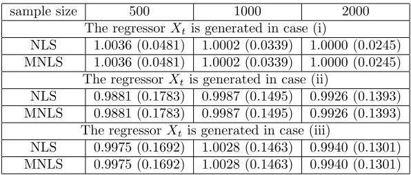
We generate 500 replicated samples for this simulation study, and cal-culate the means and standard errors for both of the parametric estima-tors in 500 simulations. In the MNLS estimation procedure, we choose Mn=Cαn1−β withα = 0.01, where Cα is defined in (3.20),β = 1 for case
[image:24.612.156.454.384.511.2](i), andβ= 1/2 for cases (ii) and (iii). It is easy to find that C0.01= 2.58.
Table 5.1. Means and standard errors for the estimators in Example 5.1
sample size 500 1000 2000
The regressorXt is generated in case (i)
NLS 1.0036 (0.0481) 1.0002 (0.0339) 1.0000 (0.0245) MNLS 1.0036 (0.0481) 1.0002 (0.0339) 1.0000 (0.0245)
The regressorXt is generated in case (ii)
NLS 0.9881 (0.1783) 0.9987 (0.1495) 0.9926 (0.1393) MNLS 0.9881 (0.1783) 0.9987 (0.1495) 0.9926 (0.1393)
The regressorXtis generated in case (iii)
NLS 0.9975 (0.1692) 1.0028 (0.1463) 0.9940 (0.1301) MNLS 0.9975 (0.1692) 1.0028 (0.1463) 0.9940 (0.1301)
The simulation results are reported in Table 5.1, where the numbers in the parentheses are the standard errors of the NLS (or MNLS) estimator in the 500 replications. From Table 5.1, we have the following interesting findings. (a) The parametric estimators perform better in the stationary case (i) than in the nonstationary cases (ii) and (iii). This is consistent with the asymptotic results obtained in Section 3.1 such as Theorem 3.1 and Corollaries 3.1 and 3.2, which indicate that the convergence rates of the parametric estimators can achieveOP(n−1/2) in the stationary case, but
onlyOP(n−1/4) in the 1/2-null recurrent case. (b) The finite sample behavior
0.01 means little sample information is lost. (c) Both of the two parametric estimators improve as the sample size increases. (d) In addition, for case (i), the ratio of the standard errors between 500 and 2000 is 1.9633 (close to the theoretical ratio√4 = 2); for case (iii), the ratio of the standard errors between 500 and 2000 is 1.3005 (close to the theoretical ratio 41/4 = 1.4142). Hence, this again confirms that our asymptotic theory is valid.
Example5.2. Consider the quadratic regression model defined by (5.2) Yt=θ0Xt2+et, θ0 = 0.5, t= 1,2,· · · , n,
where{Xt} is generated either by one of the three Markov processes
intro-duced in Example 5.1, or by (iv) the unit root process: Xt=Xt−1+xt, xt= 0.2xt−1+vt,
in whichX0 =x0 = 0,{vt}is a sequence of i.i.d.N(0,0.75) random variables,
and the error process {et} is defined as in Example 5.1. In this simulation
study, we are interested in the finite sample behavior of the MNLS estimator to illustrate the asymptotic theory developed in Section 3.2 as the regression function in (5.2) is asymptotically homogeneous. For the comparison pur-pose, we also investigate the finite sample behavior of the NLS estimation, although we do not establish the related asymptotic theory under the frame-work of null recurrent Markov chains. The sample sizenis chosen to be 500, 1000 and 2000 as in Example 5.1 and the replication number is R = 500. In the MNLS estimation procedure, as in the previous example, we choose Mn= 2.58n1−β, where β= 1 for case (i), and β = 1/2 for cases (ii)–(iv).
The simulation results are reported in Table 5.2, from which, we have the following conclusions. (a) For the regression model with asymptotically homogeneous regression function, the parametric estimators perform better in the nonstationary cases (ii)–(iv) than in the stationary case (i). This finding is consistent with the asymptotic results obtained in Sections 3.2 and 4.2. (b) The MNLS estimator performs as well as the NLS estimator (in particular for the nonstationary cases). Both the NLS and MNLS estimations improve as the sample size increases.
sample size 500 1000 2000 The regressorXtis generated in case (i)
NLS 0.5002 (0.0095) 0.4997 (0.0068) 0.4998 (0.0050) MNLS 0.5003 (0.0126) 0.4998 (0.0092) 0.4997 (0.0064)
The regressor Xtis generated in case (ii)
NLS 0.5000 (2.4523×10⁻⁴) 0.5000 (6.7110
×10−5) 0.5000 (2.7250
×10−5)
MNLS 0.5000 (2.4523×10⁻⁴) 0.5000 (6.7112
×10−5) 0.5000 (2.7251
×10−5)
The regressor Xtis generated in case (iii)
NLS 0.5000 (2.6095×10⁻⁴) 0.5000 (8.4571
×10−5) 0.5000 (3.1268
×10−5)
MNLS 0.5000 (2.6095×10⁻⁴) 0.5000 (8.4572
×10−5) 0.5000 (3.1268
×10−5)
The regressorXt is generated in case (iv)
NLS 0.5000 (2.1698×10⁻⁴
) 0.5000 (7.1500×10⁻⁵
) 0.5000 (2.6017×10⁻⁵
) MNLS 0.5000 (2.1699×10⁻⁴) 0.5000 (7.1504
×10−5) 0.5000 (2.6017
×10−5)
6. Empirical application. In this section we give an empirical appli-cation of the proposed parametric model and estimation methodology.
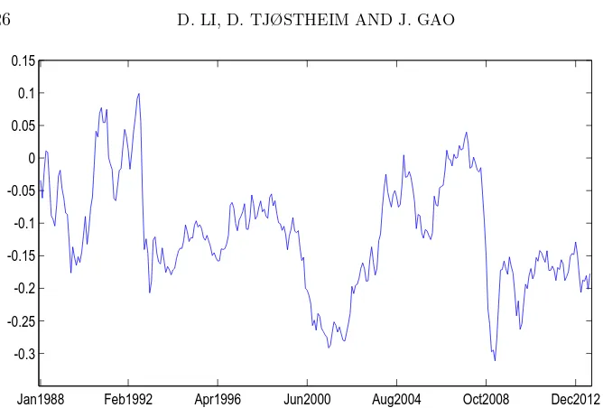
Example 6.1. Consider the logarithm of the UK to US export and import data (in£). These data come from the website: https://www.uktradeinfo.com/, spanning from January 1996 to August 2013 monthly and with the sample sizen= 212. LetXtbe defined as log(Et)+log(ptU K)−log(pU St ), where{Et}
is the monthly average of the nominal exchange rate, and {pi
t} denotes the
consumption price index of country i. In this example, we let {Yt} denote
the logarithm of either the export or the import value.
The dataXtandYtare plotted in Figures 6.1 and 6.2, respectively.
Mean-while, the real data application considered by Gaoet al(2013) suggests that
{Xt} may follow the threshold autoregressive model proposed in that
pa-per, which is shown to be a 1/2-null recurrent Markov process. Furthermore, an application of the estimation method by (3.6) gives β0 = 0.5044. This further supports that{Xt} roughly follows aβ-null recurrent Markov chain
withβ = 1/2.
To avoid possible confusion, letYex,t and Yim,t be the export and import
data, respectively. We are interested in estimating the parametric relation-ship betweenYex,t (or Yim,t) and Xt. In order to find a suitable parametric
relationship, we first estimate the relationship nonparametrically based on Yex,t =mex(Xt) +et1 and Yim,t= mim(Xt) +et2 (c.f., Karlsenet al 2007), wheremex(·) and mim(·) are estimated by
(6.1)
b
mex(x) =
Pn
t=1K Xth−x
Yex,t
Pn
t=1K Xth−x
and mbim(x) =
Pn
t=1K Xth−x
Yim,t
Pn
t=1K Xth−x
Jan1988 Feb1992 Apr1996 Jun2000 Aug2004 Oct2008 Dec2012 -0.3
[image:27.612.130.464.86.317.2]-0.25 -0.2 -0.15 -0.1 -0.05 0 0.05 0.1 0.15
Figure 6.1: Plot of the real exchange rateXt.
where K(·) is the probability density function of the standard normal dis-tribution and the bandwidthh is chosen by the conventional leave-one-out cross-validation method. Then, a parametric calibration procedure (based on the preliminary nonparametric estimation) suggests using a third-order polynomial relationship of the form
(6.2) Yex,t=θex,0+θex,1Xt+θex,2Xt2+θex,3Xt3+eex,t
for the export data, where the estimated values (by using the method in Sec-tion 3.2) of θex,0, θex,1, θex,2 andθex,3 are 21.666, 5.9788, 60.231 and 139.36, respectively, and
(6.3) Yim,t=θim,0+θim,1Xt+θim,2Xt2+θim,3Xt3+eim,t
for the import data, where the estimated values ofθim,0, θim,1, θim,2andθim,3 are 21.614, 3.5304, 37.789 and 87.172, respectively. Their plots are given in Figures 6.3 and 6.4, respectively.
Jan199620 May2000 Oct2004 Feb2005 Aug2013 20.5
21 21.5 22 22.5 23
[image:28.612.131.472.102.324.2]log(UK to USA export (value£)) log(UK to USA import (value£))
Figure 6.2: Plot of the logarithm of the export and import dataYt.
−0.3 −0.25 −0.2 −0.15 −0.1 −0.05 0 0.05
21.1 21.2 21.3 21.4 21.5 21.6 21.7 21.8 21.9 22 22.1
Figure 6.3: Plot of the polynomial model fitting (6.2).
relationship among the export or the import variable with the exchange rate and some other macroeconomic variables.
[image:28.612.130.466.341.547.2]−0.3 −0.25 −0.2 −0.15 −0.1 −0.05 0 0.05 21.1
[image:29.612.130.466.87.318.2]21.2 21.3 21.4 21.5 21.6 21.7 21.8 21.9 22
Figure 6.4: Plot of the polynomial model fitting (6.3).
that the nonstationary null recurrent process considered in this paper is un-der Markov perspective, which, unlike PP, indicates that our methodology has the potential of being extended to the nonlinear autoregressive case. In this paper, we not only develop an asymptotic theory for the NLS es-timator of θ0 when g(·,·) is integrable, but also propose using a modified version of the conventional NLS estimator for the asymptotically homoge-neous g(·,·) and adopt a novel method to establish an asymptotic theory for the proposed modified parametric estimator. Furthermore, by using the log-transformation, we discuss the estimation of the parameter vector in a conditional volatility function. We also apply our results to the nonlinear regression withI(1) processes which may be non-Markovian, and establish an asymptotic distribution theory, which is comparable to that obtained by PP. The simulation studies and empirical applications have been provided to illustrate our approaches and results.
2011. The authors acknowledge the financial support from the Norwegian Research Council. The first author was partly supported by an Australian Research Council Discovery Early Career Researcher Award (DE120101130). The third author was supported by two Australian Research Council Dis-covery Grants under Grant Numbers: DP130104229 & DP150101012.
Appendix A: Outline of the main proofs
In this appendix, we outline the proofs of the main results in Section 3. The detailed proofs of these results are given in Appendix C of the supplemental doc-ument. The major difference between our proof strategy and that based on the unit root framework (c.f., PP and Kristensen and Rahbek, 2013) is that our proofs rely on the limit theorems for functions of the Harris recurrent Markov process (c.f., Lemmas A.1 and A.2 below) whereas PP and Kristensen and Rahbek (2013)’s proofs use the limit theorems for integrated time series. We start with two technical lemmas which are crucial for the the proofs of Theorems 3.1 and 3.2. The proofs for these two lemmas are given in Appendix D of the supplemental document by Li, Tjøstheim and Gao (2015).
Lemma A.1. Let hI(x,θ) be a d-dimensional integrable function on Θ and
suppose that Assumption 3.1(i) is satisfied for{Xt}.
(a) Uniformly forθ∈Θ, we have
(A.1) 1
N(n)
n
X
t=1
hI(Xt,θ) =
Z
hI(x,θ)πs(dx) +oP(1).
(b) If{et} satisfies Assumption 3.1(ii), we have, uniformly for θ∈Θ,
(A.2)
n
X
t=1
hI(Xt,θ)et=OP
p
N(n).
Furthermore, ifR hI(x,θ0)hIτ(x,θ0)πs(dx)is positive definite, we have
(A.3) p 1
N(n)
n
X
t=1
hI(Xt,θ0)et d
−→N 0d, σ2
Z
hI(x,θ0)hτI(x,θ0)πs(dx)
.
Lemma A.2. Let hAH(x,θ) be a d-dimensional asymptotically homogeneous
function on Θ with asymptotic order κ(·) (independent of θ) and limit homoge-neous functionhAH(·,·). Suppose that{Xt}is a null recurrent Markov process with
the invariant measure πs(·)and Assumption 3.3(iv) are satisfied, andhAH(·,θ)is
continuous on the interval[−1,1]for allθ∈Θ. Furthermore, letting
∆AH(n,θ) = [Mn]
X
i=0
hAH(
i Mn
,θ)hτAH(
i Mn
,θ)πs(Bi+1(1)) +
[Mn] X
i=0
hAH(−
i Mn,
θ)hτAH(−
i Mn,
with Bi(1) andBi(2) defined in Section 3.2, there exist a continuous and positive
definite matrix∆AH(θ)and a sequence of positive numbers {ζAH(Mn)} such that
ζ0(Mn)/ζAH(Mn) is bounded, ζ0(ln)/ζ0(Mn) =o(1) for ln → ∞ but ln =o(Mn),
and
lim
n→∞
1
ζAH(Mn)
∆AH(n,θ) =∆AH(θ),
whereζ0(·)is defined in Section 3.2.
(a) Uniformly forθ∈Θ, we have
(A.4) [N(n)JAH(n,θ)] −1
n
X
t=1
hAH(Xt,θ)hτAH(Xt,θ)I(|Xt| ≤Mn) =Id+oP(1),
whereJAH(n,θ) =κ2(Mn)ζAH(Mn)∆AH(θ).
(b) If{et} satisfies Assumption 3.1(ii), we have, uniformly for θ∈Θ,
(A.5) J−AH1/2(n,θ)
n
X
t=1
hAH(Xt,θ)I(|Xt| ≤Mn)et=OP
p
N(n),
and furthermore
(A.6) N−1/2(n)J−1/2 AH (n,θ0)
n
X
t=1
hAH(Xt,θ0)I(|Xt| ≤Mn)et d
−→N 0d, σ2Id
.
Proof of Theorem3.1. For Theorem 3.1(a), we only need to verify the fol-lowing sufficient condition for the weak consistency (Jennrich, 1969): for a sequence of positive numbers{λn},
(A.7) 1
λn
Ln,g(θ)−Ln,g(θ0)=L∗(θ,θ0) +oP(1)
uniformly forθ∈Θ, whereL∗
(·,θ0) is continuous and achieves a unique minimum atθ0. This sufficient condition can be proved by using (A.1) and (A.2) in Lemma A.1, and (3.3) in Theorem 3.1(a) is thus proved. Combining the so-called Cram´er-Wold device (Billingsley, 1968) and (A.3) in Lemma A.1(b), we can complete the proof of the asymptotically normal distribution in (3.4). Details can be found in Appendix C of the supplemental document.
Proof of Corollary 3.1. The asymptotic distribution (3.7) can be proved
by using (3.5) and Theorem 3.1(b).
Proof of Theorem3.2. The proof is similar to the proof of Theorem 3.1 above. To prove the weak consistency, similar to (A.7), we need to verify the sufficient condition: for a sequence of positive numbers{λ∗
n},
(A.8) 1
λ∗ n
Qn,g(θ)−Qn,g(θ0)=Q∗(θ,θ0) +oP(1)
uniformly for θ ∈ Θ, where Q∗(
·,θ0) is continuous and achieves a unique mini-mum at θ0. Using Assumption 3.3(ii) and following the proofs of (A.4) and (A.5) in Lemma A.2 (see Appendix D in the supplemental document), we may prove (A.8) and thus the weak consistency result (3.14). Combining the Cram´er-Wold de-vice and (A.6) in Lemma A.2(b), we can complete the proof of the asymptotically normal distribution forθn in (3.15). More details are given in Appendix C of the
supplemental document.
Proof of Corollary3.3. By using Theorem 3.2(b) and (2.3), and following the proof of Lemma A.2 in Gaoet al(2014), we can directly prove (3.17).
Proof of Corollary3.4. The convergence result (3.18) follows from (3.17) in Corollary 3.3 and (3.19) can be proved by using (3.15) in Theorem 3.2(b).
SUPPLEMENTARY MATERIAL
Supplement to “Estimation in Nonlinear Regression with Harris Re-current Markov Chains”. We provide some additional simulation studies, the detailed proofs of the main results in Section 3, the proofs of Lemmas A.1 and A.2 and Theorem 4.1.
References.
[1] Bandi, F. and Phillips, P. C. B.(2009). Nonstationary continuous-time processes.
Handbook of Financial Econometrics (Edited by Y. A¨ıt-Sahalia and L. P. Hansen), Vol1, 139–201.
[2] Bec, F., Rahbek, A. and Shephard, N. (2008). The ACR model: a multivariate dynamic mixture autoregression.Oxford Bulletin of Economics and Statistics70,
583-618.
[3] Billingsley, P.(1968).Convergence of Probability Measures. Wiley, New York. [4] Chan, N. and Wang, Q. (2012). Nonlinear cointegrating regressions with
nonsta-tionary time series. Working paper, School of Mathematics, University of Sydney. [5] Chen, L., Cheng, M. and Peng, L.(2009). Conditional variance estimation in
het-eroscedastic regression models.Journal of Statistical Planning and Inference139, 236–
245.
[7] Chen, X.(1999). How often does a Harris recurrent Markov chain occur ?Annals of Probability 27, 1324–1346.
[8] Chen, X. (2000). On the limit laws of the second order for additive functionals of Harris recurrent Markov chains.Probability Theory and Related Fields116, 89–123.
[9] Gao, J. (2007).Nonlinear Time Series: Semi– and Non–Parametric Methods. Chap-man & Hall/CRC.
[10] Gao, J., Kanaya, S., Li, D. and Tjøstheim, D. (2014). Uniform consistency for nonparametric estimators in null recurrent time series. Forthcoming in Econometric Theory.
[11] Gao, J., Tjøstheim, D. and Yin, J.(2013). Estimation in threshold autoregression models with a stationary and a unit root regime.Journal of Econometrics172, 1-13.
[12] Hall, P. and Heyde, C. (1980). Martingale Limit Theory and Its Applications. Academic Press, New York.
[13] Han, H. and Kristensen, D.(2014). Asymptotic theory for the QMLE in GARCH-X models with stationary and nonstationary covariates.Journal of Business and Eco-nomic Statistics32, 416–429.
[14] Han, H. and Park, J.(2012). ARCH/GARCH with persistent covariate: Asymptotic theory of MLE.Journal of Econometrics167, 95–112.
[15] H¨opfner, R. and L¨ocherbach, E.(2003). Limit theorems for null recurrent Markov processes.Memoirs of the American Mathematical Society, Vol.161, Number768.
[16] Jennrich, R. I.(1969). Asymptotic properties of non-linear least squares estimation.
Annals of Mathematical Statistics40, 633–643.
[17] Karlsen, H. A. and Tjøstheim, D. (2001). Nonparametric estimation in null re-current time series.Annals of Statistics29, 372–416.
[18] Karlsen, H. A., Myklebust, T. and Tjøstheim, D.(2007). Nonparametric esti-mation in a nonlinear cointegration type model.Annals of Statistics35, 252–299.
[19] Karlsen, H. A., Myklebust, T. and Tjøstheim D. (2010). Nonparametric re-gression estimation in a null recurrent time series.Journal of Statistical Planning and Inference140, 3619–3626.
[20] Kallianpur, G. and Robbins, H. (1954). The sequence of sums of independent random variables.Duke Mathematical Journal21, 285–307.
[21] Kasahara, Y.(1984). Limit theorems for L´evy processes and Poisson point processes and their applications to Brownian excursions.Journal of Mathematics of Kyoto Uni-versity24, 521–538.
[22] Kristensen, D. and Rahbek, A. (2013). Testing and inference in nonlinear coin-tegrating vector error correction models.Econometric Theory29, 1238–1288.
[23] Lai, T. L. (1994). Asymptotic properties of nonlinear least squares estimations in stochastic regression models.Annals of Statistics22, 1917–1930.
[24] Li, D., Tjøstheim, D. and Gao, J. (2015). Supplement to “Estimation in nonlinear regression with Harris recurrent Markov chains”.
[25] Li, R. and Nie, L. (2008). Efficient statistical inference procedures for partially nonlinear models and their applications.Biometrics64, 904–911.
[26] Lin, Z., Li, D. and Chen, J. (2009). Local linear M–estimators in null recurrent time series.Statistica Sinica19, 1683–1703.
[27] Ling, S. (2007). Self-weighted and local quasi-maximum likelihood estimators for ARMA-GARCH/IGARCH models.Journal of Econometrics140, 849–873.
[28] Lu, Z. (1998). On geometric ergodicity of a non-linear autoregressive (AR) model with an autoregressive conditional heteroscedastic (ARCH) term. Statistica Sinica8,
1205–1217.