Full Terms & Conditions of access and use can be found at
http://www.tandfonline.com/action/journalInformation?journalCode=rtpg20
Download by: [University of Leeds] Date: 02 June 2016, At: 03:11
ISSN: 0033-0124 (Print) 1467-9272 (Online) Journal homepage: http://www.tandfonline.com/loi/rtpg20
Estimating Population Attribute Values in a Table:
“Get Me Started in” Iterative Proportional Fitting
Nik Lomax & Paul Norman
To cite this article:
Nik Lomax & Paul Norman (2016) Estimating Population Attribute Values in
a Table: “Get Me Started in” Iterative Proportional Fitting, The Professional Geographer, 68:3,
451-461, DOI: 10.1080/00330124.2015.1099449
To link to this article:
http://dx.doi.org/10.1080/00330124.2015.1099449
© 2016 The Author(s). Published with license by Taylor & Francis© N. Lomax and P. Norman
Published online: 10 Dec 2015.
Submit your article to this journal
Article views: 612
View related articles
Nik Lomax and Paul Norman
University of Leeds
Iterative proportionalfitting (IPF) is a technique that can be used to adjust a distribution reported in one data set by totals reported in others. IPF is used to revise tables of data where the information is incomplete, inaccurate, outdated, or a sample. Although widely applied, the IPF methodology is rarely presented in a way that is accessible to nonexpert users. This articlefills that gap through discussion of how to operationalize the method and argues that IPF is an accessible and transparent tool that can be applied to a range of data situations in population geography and demography. It offers three case study examples where IPF has been applied to geographical data problems; the data and algorithms are made available to users as supplementary material. Key Words: controls and constraints, interaction matrix, iterative proportionalfitting (IPF), population estimation.
迭代比例拟合方法(IPF)是一个可透过其他报告的总数来调整其中一个数据集所报告的分佈之方法。IPF用来修订信息不完
全、不正确、过时的数据表或样本。儘管 IPF 的方法受到广泛的应用,但却鲜少以非专业使用者可获得的方式呈现之。本 文透过探讨如何操作该方法来填补上述阙如, 并主张 IPF 是可被应用于人口地理学与人口学的广泛数据情境的可取得且清 晰易懂的工具。本文提供三个案例研究, 其中 IPF 被应用于地理数据问题;数据及演算法则可让使用者取得作为补充的材 料。关键词:控制与限制,互动矩阵,迭代比例拟合方法(IPF),人口估计。
El ajuste proporcional iterativo (IPF) es una tecnica que puede usarse para ajustar una distribucion reportada en un conjunto de datos por los totales reportados en otros. El IPF se usa para revisar las tablas de datos donde la informacion esta incompleta, es inexacta, obsoleta, o es una muestra. Si bien es de amplia aplicacion, la metodología IPF raramente se presenta de una manera accesible para usuarios que no sean expertos. Este artículo llena ese vacío mediante discusion sobre como operacionalizar el metodo y arguye que el IPF es una herramienta accesible y transparente que puede aplicarse a un abanico de situaciones de datos en geografía de la poblacion y demografía. El artículo presenta el ejemplo de tres estudios de caso donde el IPF se aplico a problemas de datos geograficos; los datos y los algoritmos se hacen accesibles para usuarios como material suplementario.
Palabras clave: controles y obstaculos, matriz de interaccion, ajuste proporcional iterativo (IPF), c alculo de la poblacion.
T
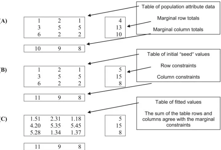
here are various data situations in population geography and demography when values for population attributes for areas might be missing due to being unknown, unreliable, outdated, or a sample. This article provides a guide to using iterative propor-tionalfitting (IPF) as a tool for estimating the missing values for these population attributes and makes the case for it as a practical technique for answering a range of research questions. Although IPF is used widely in demographic analysis, the method is rarely presented in a way that is easily reproduced and, as a result, it can be opaque to nonexpert users. The aim of this article is to highlight that IPF is a technique that can be readily applied to a variety of data and scenarios and to provide researchers new to this technique with an introductory guide and an awareness of tools they can use to apply IPF in their own work.To set the scene and introduce relevant terminol-ogy, Figure 1A shows a table of cells that are counts of
people with a specific attribute. Each table row has data for an area and each column has counts of a par-ticular population attribute in each area. External to the table are marginal cells: row totals of the number of people in each area and column totals of the popula-tion attribute across all areas. In Figure 1A, the sums of the rows and columns within the table agree with the marginal row and column totals. Supposing data for a subsequent year became available, but only the total population in each area (the row totals) and the population attribute totals for the large area, these smaller areas comprise (the column totals). This is the situation in Figure 1B, but the sum of the rows and columns of the table cells no longer agree with the external marginal cells. Using the internal table cell values as initial or“seed”values, IPF can be used to constrain (control or scale) the table tofit the marginal totals. Once IPF has been implemented, in Figure 1C, the internal values in the table now sum to the
© N. Lomax and P. Norman
This is an Open Access article distributed under the terms of the Creative Commons Attribution License (http://creativecommons.org/licenses/by/3.0), which permits unrestricted use, distribution, and reproduction in any medium, provided the original work is properly cited. The moral rights of the named author(s) have been asserted.
The Professional Geographer, 68(3) 2016, pages 451–461
Initial submission, April 2015; revised submission, August 2015;final acceptance, August 2015. Published with license by Taylor & Francis Group, LLC.
marginal row and column constraints and the data sets are said to have converged.
Following a brief discussion on the background of IPF, its previous applications, and some analogous methods, this article goes on to step through the IPF procedure and offer some pointers on operationalizing the algorithm. It then offers discussion of software implementation and applies the IPF method to three practical case study examples: estimating populations by age and sex, estimating migration flows between areas, and estimating multiple attributes for local area populations using a sample distribution. Finally, some conclusions are offered. The following section serves to highlight that although IPF is a widely used tech-nique, the extant literature is not particularly useful for the casual user or someone new to IPF.
Background of IPF
IPF has been used in a wide variety of applications from multiple disciplines and the technique is referred to by various names: RAS in economics (from the notation of the model^rA^s; see Bacharach 1965),Cross– Fratar (Fratar 1954) or Furness (Furness 1965) in transport engineering, andrakingin computer science and statistics (Cohen 2008). IPF has also been referred to as rim-weighting or structure-preserving estimation (Simpson and Tranmer 2005). Johnston and Pattie (1993, 317) pointed toward a large body of literature in the field of geography that deals with approaches
that are “entropy-maximizing, based on maximum likelihood estimation for which the IPF procedure is a means to that end.”We discuss other equivalent meth-ods that aim to achieve maximum likelihood in the next section. In demographics, thefirst use of IPF is widely attributed to Deming and Stephan (1940), who applied the technique to data from the 1940 U.S. cen-sus of population. Deming and Stephan found that although there were complete counts of the popula-tion for certain characteristics, when these characteris-tics were cross-tabulated the output was limited to a sample of the population. They used this sample as the starting distribution (the seeds) and applied IPF to derive an estimate of these cross-tabulated characteris-tics for the whole population. The ideas presented in Deming and Stephan (1940) were further explored and discussed by Deming (1943), Bishop (1969), Friedlander (1961), and Fienberg (1970), to name just a few. Many of these early papers, being presented from a mathematician’s perspective, however, are likely to be incomprehensible to nonspecialist audien-ces and do not step through the proaudien-cess of using IPF such that somebody new to the technique could emu-late it in similar settings.
[image:3.504.78.437.45.290.2]More recent demographic applications of IPF cover a variety of data sets and data availability and reliability issues. At the microdata level, Birkin and Clarke (1988) used IPF to estimate the characteristics of resi-dents of small geographical areas, Rees (1994) updated the age and sex structure of small area populations, and Pritchard and Miller (2012) assigned multiple Figure 1Data framework and terminology.
attributes to a synthetic population as an input to a microsimulation model. Simpson and Tranmer (2005) scaled small area population counts to large area infor-mation, using IPF to estimate a cross-tabulation of car ownership and tenure type using 1991 Census data. Lomax et al. (2013) used IPF to estimate missing migration data for the United Kingdom, and aggregate migration data were disaggregated by age and sex by Willekens, Por, and Raquillet (1981) and Willekens (1982).
Although all of these papers have applied IPF effec-tively to specific data problems, none are designed to guide the reader through the process of estimating the required information; rather, they present the tool as a means of getting at the results. Clearer explanations of IPF as a technique are offered by Wong (1992) and Rees (1994), but both are still opaque to those strug-gling with algebra. One exception is Norman (1999), who provided a guide on IPF but still without a step-through of the calculations involved. For a comprehen-sive history, summary of various applications, and detailed discussion on the robustness of IPF, see Zaloznik (2011).
Analogous Methods
IPF is not the only method that can be used for com-bining population data and estimating missing values. For example, in population estimation, the apportion-ment method can be used to ensure that small area data are made consistent with larger area information and the ratio method to update earlier cell counts. Both the apportionment and ratio methods can be regarded as ways of scaling data so that one source agrees with another. For definitions of these methods, see Rees, Norman, and Brown (2004). When estimat-ing a contestimat-ingency table of migration data, linear regression models are often the method of choice, in the form of Poisson regression models (Boyle 1993; Bohara and Krieg 1996) or log-linear regression mod-els (Rogers, Little, and Raymer 2010; Raymer, de Beer, and van der Erf 2011). Similarly, spatial interac-tion models have a well-established place in the estima-tion of interacestima-tion data (Rees, Fotheringham, and Champion 2004; Congdon 2010) with a very useful introduction provided by Dennett (2012). When esti-mating a multidimensional age by sex by origin by des-tination table, van Imhoff et al. (1997) experimented with both log-linear modeling and IPF. They found that thefitted rates from the two methods are the same but favored IPF for its efficiency and speed.
For creating small area synthetic populations with multiple attributes, IPF is compared to hill climbing algorithms by Kurban et al. (2011) and to the combi-natorial optimization (CO) method by Ryan, Maoh, and Kanaroglou (2009). The hill climbing algorithms are used by Kurban et al. (2011) to create cross-tabula-tions of households where only univariate distribucross-tabula-tions are available by swapping households within a
randomly generated distribution until this distribution matches the real marginal totals. The CO method used by Ryan, Maoh, and Kanaroglou (2009) builds a syn-thetic population by swapping individuals until they closely match an observed distribution. Both studies found IPF a capable tool for the job but stated a prefer-ence for the analogous method due to improved accu-racy. Both acknowledged, however, that their conclusions were drawn from the estimation of rela-tively small synthetic populations and called for further research on larger synthetic populations. These exam-ples demonstrate that choosing a method (IPF or another) is largely down to the preferences of the researcher, the data problem being investigated, and the resources (time, software, and skills) available.
An Example of the IPF Algorithm
In this section we explain the steps involved in implement-ing IPF and how the values in Figure 1B became thefitted values in Figure 1C. Table 1 begins with the initial seed values at what is referred to as Step 0, along with the sum of the table rows and columns and the marginal row and column constraints. Note that values are reported to two decimal places. The mathematical equations for the proce-dure are presented in the Appendix.
In Step 0, a table of initial seed values is available but the sum of the table rows does not equal the constraint row totals and the sum of the table columns does not equal the column constraint totals. IPF will adjust the table seed values to agree with both the row and col-umns constraints.
IPF proceeds as follows. In Step 1a, the values within the table are scaled to sum to the row constraints. The top left cell in Step 1a is calculated as 1.25D1.00 * 5.00/4.00 where 1.00 is the initial seed value, 5.00 is the row constraint, and 4.00 is the sum of the table row values in Step 0. The first cell in the middle row of Step 1a is calculated as 3.46, taking the values from Step 0 of 3.00 in the table, multiplied by the row con-straint (15.00) divided by the table row sum (13.00). All other cells are calculated accordingly and at the end of Step 1a, the sum of each table row equals the row con-straint. The sum of the table columns is different to that at Step 0 but still does not sum to the column constraint.
Step 1b then adjusts the table cell counts in Step 1a to agree with the constraint column totals. The top left cell in the table in Step 1b is calculated using values from Step 1a so that 1.45 D1.25 * 11.00/9.51. The next cell down is calculated as 4.00D3.46 * 11.00/9.51 and the bottom cell 5.55 as 4.80 * 11.00/9.51. The other table cells are scaled similarly so that the sum of the table columns now agrees with the column con-straints. Although the sum of the table rows agreed with the row constraints at the end of Step 1a, this is no longer the case. At the end of Step 1b, one iteration is complete. Because the difference between the row totals and the row constraints is larger than the
predefined threshold (here 0.01), we go back to Step 1 and begin the next iteration. This predefined thresh-old (convergence) is user specified and can be mea-sured by individual row and column differences or by the difference between the row and column totals.
Step 2 is the next iteration. In Step 2a, the values in the table at Step 1b are scaled so that they sum to the row constraints. The top left cell in Step 2a is 1.48, calculated as 1.45 * 5.00/4.89, with equivalent calcula-tions carried out for all the cells in the table. The table row totals now sum to the row constraints but the
table column totals do not agree with the column con-straints. In Step 2b, the top left cell is 1.50 calculated from the values in Step 2a, 1.48 * 11.00/10.81 and all the other table cell values accordingly. Once the table values have been controlled to sum to the column con-straints, the table row totals do not sum to the row constraints (but the difference is not as large as at the end of thefirst iteration at Step 1b).
The IPF routine then proceeds by alternating the scal-ing of the table cell values to agree with the row constraints and then to the column constraints. The Table 1 A step-through of the iterative proportional fitting calculation
Step 0 Table initial seed values 1.00 2.00 1.00 4.00 5.00 3.00 5.00 5.00 13.00 15.00 6.00 2.00 2.00 10.00 8.00 Table column totals 10.00 9.00 8.00 Table row totals Constraint row Constraint column totals 11.00 8.00 9.00 totals
Step 1a Scale Step 0 table values to agree with row constraints
1.25D1.00* (5.00/4.00)
2.50D2.00* (5.00/4.00)
1.25D1.00* (5.00/4.00)
5.00 5.00
3.46D3.00* (15.00/13.00)
5.77D5.00* (15.00/13.00)
5.77D5.00* (15.00/13.00)
15.00 15.00
4.80D6.00* (8.00/10.00)
1.60D2.00* (8.00/10.00)
1.60D2.00* (8.00/10.00)
8.00 8.00
Table column totals 9.51 9.87 8.62 Table row totals Constraint row Constraint column totals 11.00 8.00 9.00 totals
Step 1b Scale Step 1a values to agree with column constraints
1.45D1.25* (11.00/9.51)
2.03D2.50* (8.00/9.87)
1.31D1.25* (9.00/8.62)
4.78 5.00
4.00D3.46* (11.00/9.51)
4.68D5.77* (8.00/9.87)
6.02D5.77* (9.00/8.62)
14.70 15.00
5.55D4.80* (11.00/9.51)
1.30D1.60* (8.00/9.87)
1.67D1.60* (9.00/8.62)
8.52 8.00
Table column totals 11.00 8.00 9.00 Table row totals Constraint row Constraint column totals 11.00 8.00 9.00 totals
Step 2a Scale Step 1b table values to agree with row constraints
1.48D1.45* (5.00/4.89)
2.33D2.28* (5.00/4.89)
1.19D1.16* (5.00/4.89)
5.00 5.00
4.11D4.00* (15.00/14.62)
5.40D5.26* (15.00/14.62)
5.49D5.35* (15.00/14.62)
15.00 15.00
5.23D5.55* (8.00/8.50)
1.37D1.46* (8.00/8.50)
1.49D5.55* (8.00/8.50)
8.00 8.00
Table column totals 10.81 9.11 8.08 Table row totals Constraint row Constraint column totals 11.00 8.00 9.00 totals
Step 2b Scale Step 2a values to agree with column constraints
1.50D1.48* (11.00/10.81)
2.31D2.33* (9.00/9.11)
1.18D1.19* (8.00/8.08)
4.99 5.00
4.18D4.11* (11.00/10.81)
5.34D5.40* (9.00/9.11)
5.44D5.49* (8.00/8.08)
14.95 15.00
5.32D5.23* (11.00/10.81)
1.36D1.37* (9.00/9.11)
1.49D1.19* (8.00/8.08)
8.06 8.00
Table column totals 11.00 8.00 9.00 Table row totals Constraint row Constraint column totals 11.00 8.00 9.00 totals
Step Xa Scale Step 2b table values to agree with row constraints
1.55D1.55* (5.00/5.00)
2.10D2.10* (5.00/5.00)
1.36D1.36* (5.00/5.00)
5.00 5.00
4.18D4.18* (15.00/14.99)
4.72D4.71* (15.00/14.99)
6.10D6.10* (15.00/14.99)
15.00 15.00
5.27D5.28* (8.00/8.01)
1.19D1.19* (8.00/8.01)
1.54D1.54* (8.00/8.01)
8.00 8.00
Table column totals 11.00 8.00 9.00 Table row totals Constraint row Constraint column totals 11.00 8.00 9.00 totals
Step Xb Scale Step Xa values to agree with column constraints
1.55D1.55* (11.00/11.00)
2.10D2.10* (9.00/9.00)
1.36D1.36* (8.00/8.00)
5.00 5.00
4.18D4.18* (11.00/11.00)
4.72D4.72* (9.00/9.00)
6.10D6.10* (8.00/8.00)
15.00 15.00
5.27D5.27* (11.00/11.00)
1.19D1.19* (9.00/9.00)
1.54D1.54* (8.00/8.00)
8.00 8.00
Table column totals 11.00 8.00 9.00 Table row totals Constraint row Constraint column totals 11.00 8.00 9.00 totals
difference between the newly calculated rows and columns and the original constraints gets closer with every iteration. The IPF routine continues through the iteration process until Step X. Once the alternate constraints have been applied several times, the table cell values sum to agree with both the row and column marginal constraints. This is the case in Step Xb and the iterations stop.
There is a formal test for whether the table valuesfit the constraints (e.g., because the preceding data are only shown to two decimal places and further precision might show that thefit is not so exact). Bishop, Fien-berg, and Holland (1975) discussed the convergence of the procedure and stopping rules. Convergence has occurred and the procedure stops when no cell value would change in the next iteration by more than a pre-defined amount that obtains the desired accuracy. A straightforward way to test for convergence is to carry out an iteration and to calculate the absolute difference between the tables generated by the row and the col-umn constraints. Then,find the maximum value of the absolute differences and check this against the required convergence value.
IPF: Further Aspects
Here weflag some elements to be aware of when pre-paring data for use in and operationalizing IPF. For the marginal constraints, the sum of the row con-straints must equal the sum of the column concon-straints and be of the same data type (i.e., counts, proportions); otherwise, IPF will not converge. Lomax et al. (2013) outlined a method for adjusting row constraints to agree with column constraints where the differences are small. There might be issues with using noninteger constraints in some programming languages (e.g., Visual Basic for Applications [VBA]), due to the way that the double data type is handled. Lovelace and Bal-las (2013) offered some advice on creating integer weights. Many formulations of the IPF algorithm do not deal well with zero values in the constraints because there would be divisions by zero (although there are some exceptions; see, e.g., Dennett’s [2011] Desktop IPF program). A simple solution to this prob-lem is to add a small constant (e.g., 0.0001). There can be no negative values because the scaling leads to strange results.
For the initial table seed values, avoid having zero values in the table. Bishop et al. (1975, 101) noted that “too many”zero cells in the initial matrix might prevent con-vergence through a“persistence of zeros.”Norman (1999) noted that“too many”is undefined, but in practice this is found to be around 30 percent of the values within the seed table if they are distributed evenly, or around 10 per-cent if the zeros are clustered together. The simplest way to allow for a large number of zero cells in the initial matrix is to add a small constant (less than the convergence test value) to all cells.
A convergence test value needs to be chosen that is appropriate to the data being used, the application, and the
precision needed. It could be that for population-related data, the nearest 0.5 person is adequate. Setting a conver-gence value that is very low will result in more iterations, so it is important to weigh up the requirements for accu-racy against time and computational aspects. Note that it is also possible to specify the maximum number of iterations, so the procedure will end before the convergence value is reached.
Expansion to Three and Four Dimensions
The example presented in the previous section can be referred to as two-dimensional (2D) IPF where the row and column margins represent two one-dimen-sional variables (e.g., these could be sex by age). IPF can be expanded to include three dimensions (3D) or evenndimensions (nD) when additional variables are included in the adjustment (e.g., age group by sex by ethnic group would require a 3D IPF solution). Deming and Stephan (1940) referred to the third dimension as a slice. For 3D IPF, the three margins (column, row, and slice) can be one-dimensional varia-bles of age, sex, and ethnicity, respectively, or combi-nations of these, so age by sex, age by ethnicity, and sex by ethnicity, for example. As with the 2D example, these margins must all sum to the same value. The third dimension is often geography, as is the case in Simpson and Tranmer (2005), and the method is used to add multiple population attributes to synthetic pop-ulations (Beckman, Baggerly, and McKay 1996; Rich and Mulalic 2012). The technical requirements and good practice set out earlier still apply when using IPF on a data set with more than two dimensions. An exam-ple of 3D IPF is presented in Case Study 3 later in this article, where the algorithm deals with three dimen-sions in the order row, column, slice.
In the next section we present three case studies that step through the implementation of IPF in different population-related data challenges. Thefirst two case studies describe the use of IPF in two dimensions; the third case study presents an example using IPF to esti-mate three dimensions of a table.
Practical Applications: Using IPF in the Real World
As a method, IPF has substantial advantages for solving real-world problems. It is fast and requires little computational power when compared with other methods (Lovelace et al. 2015); the methodology is transparent (once it is properly explained) and is repro-ducible; that is, with the same inputs, the outcome is the same no matter how many times it is implemented. There is also growing support for implementing IPF in a variety of statistical packages, discussed next. Fol-lowing that we present three case study examples, where IPF has been used to overcome some real-world data issues. Links to the supplementary materials are supplied with each of these examples.
Software for Implementing IPF
IPF can be implemented in a variety of different soft-ware packages and the choice is down to the prefer-ence of the researcher. In the examples used for this article, the estimation of populations by age and sex has been implemented using VBA in Microsoft Excel (Norman 1999), and the estimation of migrationflows and estimation of population-level attributes in two-and three-dimensional tables, respectively, have been implemented in the R software package. Modules or user-produced syntax are available for a number of other platforms, including SAS, Matlab, Stata, and SPSS. The code and datafiles used in the examples presented in this article are available at https://github. com/niklomax/IPFexamples. The IPF code used in Case Study 2 was originally developed by Tomlinson and Hunsinger for the Alaska Department of Labor and Workforce Development (2009) and is freely available for researchers to download. The code has been used by the Alaska Department of Labor and Workforce Development to integrate characteristics (e.g., race) into population totals derived from the U.S. Census Bureau. The code has also been used to estimate cyclical employment and unemployment flows in the United States by Coleman (2010) and to create cross-tabulations of area variables where only univariate distributions are available by Kurban et al. (2011). Case study 3 is implemented using the‘mipfp’ package in R.
Case Study 1: Using IPF in Population Estimates Small area population estimates by age and sex are needed to show the population size and structure and as denominators for the calculation of rates (Norman, Simpson, and Sabater 2008). Although these popula-tions are available for the midyear closest to the cen-sus, this is not necessarily the case in other years. A cohort-component method is commonly used whereby a base population by age and sex is updated to a later time point using counts of the births and deaths and the migration moves in and out of the area in the intervening period (Rees et al. 2003). Although data on births and deaths are usually available for small area geographies, the necessary migration counts are rarely obtainable. An approach that combines data sources and methods is a pragmatic solution.
Thus, for a set of small areas that comprise a larger area, a simple cohort-component method can be used to update the base populations byfive-year age and sex with allowances for births, deaths, and aging but not for migration. This can provide initial seed values for IPF to then constrain these age–sex values at small area level to be consistent with sepa-rately estimated total populations for each area and with age–sex information from the containing larger area. As an example, populations byfive-year groups for 1991 will be updated to 1996. This draws on Rees et al. (2003); Rees, Norman, and Brown
(2004); and Norman, Simpson, and Sabater (2008), including their data inputs, and will be for the local government district of Bradford, England, which includes thirty electoral wards. Official age–sex esti-mates are available for Bradford as a whole for 1996 and births and deaths occurring in each ward between 1991 and 1996. Gross migration flows in and out of each ward are not available. Total ward populations have been separately estimated using the ratio method (Rees et al. 2003), using indicators of change in overall population size (thereby includ-ing change due to migration).
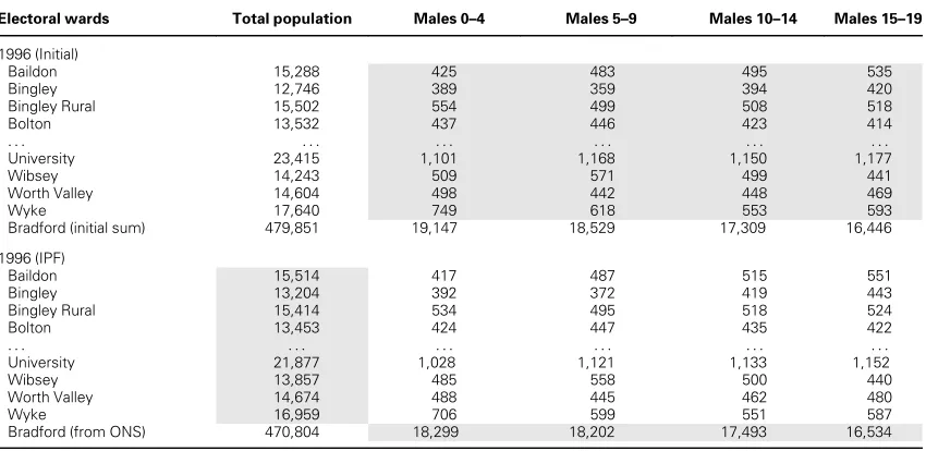
The top portion of Table 2 has the initial popula-tions for 1996 derived as just stated. Selected wards and males up to age fifteen to nineteen are shown. The full data set has males and females up to age eighty-five for all thirty wards. The sum of the age– sex information provides a total in each ward and the sum across wards provides totals for the district. These ward and district populations are different from those obtained for 1996 from the specific estimates of total populations and the official estimates for Bradford from the Office for National Statistics (ONS; bottom of Table 2). Both of these estimates include indicators of change due to migration, but the initial ward age– sex estimates do not. Table 2 has the initial estimates constrained using IPF to be consistent with the ward (row) marginal and district (column) marginals.
Population estimates are just that—estimates—and we cannot know whether they are correct. Various data sources are available to measure demographic change in an area and these all have strengths and weaknesses. Combining these sources in a way that uses their strengths and compensates for their weak-nesses makes the subsequent estimates defensible, and IPF plays a key role in this (Rees et al. 2003; Norman, Simpson, and Sabater 2008). The method outlined here has been shown to be an improvement over sim-pler methods and to perform equivalently to methods that, after time-consuming data preparation, incorpo-rate up-dated gross migrationflows based on the pre-vious census (Rees, Norman, and Brown 2004).
The case study is implemented using VBA in Microsoft Excel. The implementation has the advantage of provid-ing a clear step-through interface but lacks the ability to deal with very large data problems. For an alternative implementation of IPF in VBA, see Dennett (2011).
Case Study 2: Estimating Migration Flows Between Areas
Estimating the flow of people between one area and another is an application that is particularly suited to IPF as data sets are often available for total moves into and out of an area (i.e., the row and column con-straints) but the data for the interaction between these areas are often not available, sparse, or incomplete. Previous examples include Chilton and Poet (1973), who used IPF to estimate migration between London
boroughs reported in the 1966 Sample Census; Rees and Duke-Williams (1997), who estimated suppressed flows reported in the 1991 Census; Nair (1985), who estimated migration in India and Korea using lifetime migration tables; and Schoen and Jonsson (2003), who estimated interregional migration in the United States between 1980 and 1990.
More recently, Lomax et al. (2013) used IPF to update a seed table of Local Authority District (LAD)-level interac-tions derived from the 2001 Census for the four countries of the United Kingdom. LADs are the administrative units at which resources and funding are allocated, so a good estimate of migration is necessary to ensure the population estimates are accurate. Different statistical reporting sys-tems are in place for England, Wales, Scotland, and Northern Ireland, so Lomax et al. (2013) used IPF to pro-duce a consistent UK data set. Between censuses, the interaction data (moves between LADs) are sparse, heavily rounded for disclosure control purposes, or not available at all (in Northern Ireland and for moves between LADs located in different countries). Outside of the census (con-ducted every ten years), the only data that are consistently available are the total outmigration from an LAD to all other LADs and the total inmigration to an LAD from all other LADs, derived from National Health Service (NHS) data.
The example presented in Table 3 focuses on migration among the twenty-six LADs of Northern Ireland (for which there are no interaction data) in a single year (2001– 2002). In the Lomax et al. (2013) article the estimate is extended to incorporate moves between LADs where a migrant crosses the border from one UK country to another for each year 2001–2002 to 2010–2011.
Table 3 shows two matrices of origin–destination interaction data for moves among the twenty-six LADs for Northern Ireland, before and after the IPF routine has been applied. These matrices are collapsed and show only thefirst and last two entries in each table. The seed table (the top portion of Table 3) contains data taken from the 2001 Census for the distribution of origin–destination interactions. The vertical margin contains total outmigration from each LAD to all other LADs, whereas the horizontal margin contains inmi-gration totals. The shaded margins in the bottom portion of Table 3 show the total in- and outmigration for 2001—2002, derived from NHS data. The IPF routine is applied to the data, and after sixteen itera-tions the data converge and the seed table is adjusted to agree with both the vertical and horizontal margins. Thus, the high-level interactions between areas that are reported in the 2001 Census are maintained, but theflows that are reported in the estimated table now sum to the in- and outmigration totals reported for 2001–2002.
[image:8.504.37.462.65.272.2]Lomax et al. (2013) reported that the IPF-derived estimates are reliable and useful, especially where there are no observed data, as is the case in Northern Ire-land. This example is implemented using R code devel-oped by the Alaska Department of Labor and Workforce Development (2009). The code has the advantage of being very efficient, offers failsafe checks (e.g., ensuring column and row constraints are equal), and deals with zeros in the margin by adding a small constant (0.001). An additional step-through guide was developed by Hunsinger (2008). This R code can also deal with IPF in three and four dimensions.
Table 2Constraining initial age–sex population estimates using iterative proportional fitting
Electoral wards Total population Males 0–4 Males 5–9 Males 10–14 Males 15–19
1996 (Initial)
Baildon 15,288 425 483 495 535
Bingley 12,746 389 359 394 420
Bingley Rural 15,502 554 499 508 518
Bolton 13,532 437 446 423 414
. . . .
University 23,415 1,101 1,168 1,150 1,177
Wibsey 14,243 509 571 499 441
Worth Valley 14,604 498 442 448 469
Wyke 17,640 749 618 553 593
Bradford (initial sum) 479,851 19,147 18,529 17,309 16,446
1996 (IPF)
Baildon 15,514 417 487 515 551
Bingley 13,204 392 372 419 443
Bingley Rural 15,414 534 495 518 524
Bolton 13,453 424 447 435 422
. . . .
University 21,877 1,028 1,121 1,133 1,152
Wibsey 13,857 485 558 500 440
Worth Valley 14,674 488 445 462 480
Wyke 16,959 706 599 551 587
Bradford (from ONS) 470,804 18,299 18,202 17,493 16,534
Note:The inputs to iterative proportional fitting are the table shaded in the top section, which provides the seed values; the row marginal constraints are the shaded ward total populations and the district column marginal constraints both in the lower section. IPFDiterative pro-portional fitting; ONSDoffice for National Statistics.
Case Study 3: Analyzing General Health by Ethnic Group and Age
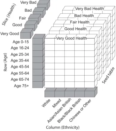
[image:9.504.42.471.71.223.2]Thisfinal case study uses IPF tofit a sampled table to three constraints derived from local area information, so it is an example of a three-dimensional application. Calculating age-specific rates of general health by eth-nic group for each local authority is useful to indicate whether there are differences in age gradients of health by ethnic group and is essential as an input to directly standardized illness measures. Data from the 2011 UK Census are available from the Local and Detailed Characteristics tables, which have cross-tabu-lations of elements of these dimensions but, even for broad ethnic groupings, without sufficient detail on age (e.g., LC2301ew, LC3206ew, DC3201ew), gen-eral health (DC3201ew), or geography (DC3204ewr). Table DC3204ewr comes closest but, due to small cell counts that result from the cross-tabulation, the data are only released at the regional and country level.
The Census Samples of Anonymised Records are individual-level microdata that have great versatility in terms of creating application-relevant recoded varia-bles and in enabling cross-tabulations not readily avail-able in the census area tavail-ables to be carried out (Norman and Boyle 2010). A 2011 Census Microdata Teaching File of an anonymized, random sample of census records was released by the Office for National Statistics to allow users to analyze census data in a way that is not possible using standard census tables. For England and Wales (i.e., with no subnational geogra-phy), a cross-tabulation of the 2011file of age (eight groups from age zero to fifteen to seventy-five and over), ethnic group (five broad groups), and general health (five levels from very good health to very bad health) can provide the initial seed values for IPF in these three dimensions.
The constraints for each LAD in England and Wales are obtained from tables QS103ew: Age; KS201ew: Ethnic group; and KS301ew: General
health. Respectively, these are the rows, columns, and slice. The data required for this adjustment can be seen in Figure 2. For each LAD in England and Wales, the number of people by ethnic group (column totals), the number of people by age (row totals), and the number of people by health (slice) are known but not the cross-tabulation between these three variables. The cross-tabulations between these variables are obtained from the microdata sample, and these form the starting seed distribution, conceptualized in Fig-ure 2 as a cube to be adjusted: age by ethnicity by very good health at the front through to age by ethnicity by very bad health at the back. The seed is adjusted and constrained to the available totals (first by age, then ethnicity, then health), and convergence occurs in
Figure 2 Iterative proportional fitting over three dimen-sions (age, ethnicity, and health).
Table 3 Data used in the iterative proportional fitting estimation of origin–destination interaction flows between Local Authority Districts in Northern Ireland: Before and after IPF
Destination
LAD 1 LAD 2 LAD. . . LAD 25 LAD 26 Outflow 2001 Census (initial)
Origin LAD 1 0 40 . . . 3 3 1,271
LAD 2 15 0 . . . 519 2 1,588 LAD. . . .
LAD 25 9 2 . . . 0 87 847 LAD 26 2 3 . . . 139 0 646 Inflow 1,270 2,184 . . . 559 375 37,437 2002 estimate (IPF)
Origin LAD 1 0.001 34.41 . . . 3.17 3.44 1,251 LAD 2 14.13 0.001 . . . 534.45 2.11 1,513 LAD. . . . LAD 25 5.77 1.12 . . . 0.001 89.39 635 LAD 26 0.01 1.91 . . . 174.35 0.001 567 Inflow 1,334 2,081 . . . 865 423 38,344 Note:The inputs to iterative proportional fitting are the table shaded in the top section, which provides the seed values from the 2001 Cen-sus; the row marginal constraints are the shaded total in- and outmigration derived from the National Health Service data, both in the lower section. The fitted table in the lower section took 16 iterations. LADDLocal Authority District; IPFDiterative proportional fitting.
[image:9.504.270.464.431.651.2]around eleven steps. This procedure is repeated for each LAD for which there are individual column, row, and slice total constraints. The constrained result pre-sumes that the same interaction between the dimen-sions exists at the local level as at the national level. In a research situation, this could be addressed by using LAD-level microdata (Office for National Statistics 2015). Using this method, a range of local area cross-tabulations can be estimated for the local and detailed characteristics tables.
The example presented here is implemented using ‘mipfp’in R, a fast and versatile package designed for the multidimensional implementation of IPF. The syn-tax supplied at https://github.com/niklomax/IPFexam ples shows how the algorithm can be implemented using very few lines of code, once an external package is relied on to undertake the calculation. Mipfp benefits from being continuously updated, has its own docu-mentation, and can be expanded to deal with problems where available constraints are cross-tabulated (age by health, age by ethnicity, ethnicity by health, etc.).
Conclusion
This article provides a how-to guide on using IPF to estimate data where information is outdated, missing, or inaccurate. It builds on and adds to existing litera-ture by providing a discussion on the practicalities of using IPF and offers a clear and jargon-explained description of how to implement the method. This article demonstrates that IPF has been used extensively in previous research as the preferred method for solv-ing real-world data problems, and we presented three case studies where IPF has been used. The diversity of issues presented in these case studies serves to high-light theflexibility of IPF as a method and its applica-bility as a research tool.
Other methods can be used to solve these data prob-lems. These are identified within the article, and we suggest that it is largely up to the researcher to decide which would be best, whether this be IPF or an analo-gous method. We make a case for choosing IPF, how-ever, and argue that IPF is a method that is transparent and computationally efficient. We also believe that IPF is a fairly simple solution to implement, which produ-ces consistent results. These outputs can be repro-duced by other users given the same inputs and we encourage readers to explore the data files and code associated with the article.
The aim of this article was to highlight the research applicability of IPF and provide researchers new to its implementation with an introductory guide and an awareness of tools they can use. The next steps in terms of advised reading would be Norman (1999), Wong (1992), and Simpson and Tranmer (2005). Comprehensive and detailed coverage is provided by Zaloznik (2011) and an overview of IPF use in geogra-phy can be found in Johnston and Pattie (1993).&
Acknowledgments
The authors are grateful to Eddie Hunsinger at the Alaska Department of Labor and Workforce Develop-ment for guidance on developing the case study mate-rial and for permission to use his R code. Thanks also for the recommendations provided by two anonymous referees. Data used in case studies are adapted from data from the Office for National Statistics and the Northern Ireland Statistics and Research Agency licensed under the Open Government Licence v.3.0.
Funding
This research was funded by an Economic and Social Research Council grant (ES/L013878/1).
Literature Cited
Alaska Department of Labor and Workforce Development. 2009. Iterative proportional fitting R code. http://www. demog.berkeley.edu/»eddieh/datafitting.html (last accessed 27 October 2015).
Bacharach, M. 1965. Estimating nonnegative matrices from marginal data.International Economic Review6 (3): 294–310. Beckman, R. J., K. A. Baggerly, and M. D. McKay. 1996.
Creating synthetic baseline populations. Transportation Research Part A: Policy and Practice30 (6): 415–29.
Birkin, M., and M. Clarke. 1988. SYNTHESIS—A synthetic spatial information system for urban and regional analysis: Methods and examples. Environment and Planning A 20 (12): 1645–71.
Bishop, Y. M. 1969. Full contingency tables, logits, and split contingency tables.Biometrics25 (2): 383–99.
Bishop, Y. M. M., S. E. Fienberg, and P. W. Holland. 1975.
Discrete multivariate analysis: Theory and practice. Cambridge, MA: MIT Press.
Bohara, A. K., and R. G. Krieg. 1996. A zero-inflated Poisson model of migration frequency.International Regional Science Review19 (3): 211–22.
Boyle, P. 1993. Modelling the relationship between tenure and migration in England and Wales.Transactions of the Institute of British Geographers18 (3): 359–76.
Chilton, R., and R. Poet. 1973. An entropy maximising approach to the recovery of detailed migration patterns from aggregate census data.Environment and Planning5 (1): 135–46.
Cohen, M. 2008. Raking. In Encyclopedia of survey research methods, ed. P. Lavrakas, 672–74. Thousand Oaks, CA: Sage. Coleman, D. 2010. Projections of the ethnic minority
populations of the United Kingdom 2006–2056.Population and Development Review36 (3): 441–86.
Congdon, P. 2010. Random-effects models for migration attractivity and retentivity: A Bayesian methodology.
Journal of the Royal Statistical Society: Series A (Statistics in Society)173 (4): 755–74.
Deming, W. E. 1943.Statistical adjustment of data. New York: Wiley. Deming, W. E., and F. F. Stephan. 1940. On a least squares adjustment of a sampled frequency table when the expected marginal totals are known. The Annals of Mathematical Statistics11 (4): 427–44.
Dennett, A. 2011. Iterative proportional nitwit. http://adam dennett.co.uk/2011/07/28/iterative-proportional-nitwit/ (last accessed 27 October 2015).
———. 2012. Estimating flows between geographical locations: “Get me started in” spatial interaction modelling. Working Paper 181, Centre for Advanced Spatial Analysis, University College, London.
Fienberg, S. E. 1970. An iterative procedure for estimation in contingency tables.Annals of Mathematical Statistics41 (3): 907–14.
Fratar, T. J. 1954. Vehicular trip distribution by successive approximations.Traffic Quarterly8 (1): 53–65.
Friedlander, D. 1961. A technique for estimating a contingency table, given the marginal totals and some supplementary data.Journal of the Royal Statistical Society: Series A (General)124 (3): 412–20.
Furness, K. P. 1965. Time function iteration. Traffic Engineering and Control7 (7): 458–60.
Hunsinger, E. 2008. Iterative proportionalfitting for a two-dimensional table. http://www.demog.berkeley.edu/
»eddieh/IPFDescription/AKDOLWDIPFTWOD.pdf (last accessed 27 October 2015).
Johnston, R., and C. Pattie. 1993. Entropy-maximising and the iterative proportionalfitting procedure.The Professional Geographer45 (3): 317–22
Kurban, H., R. Gallagher, G. A. Kurban, and J. Persky. 2011. A beginner’s guide to creating small-area cross-tabulations.
Cityscape: A Journal of Policy Development and Research13 (3): 225–35.
Lomax, N., P. Norman, P. Rees, and J. Stillwell. 2013. Subnational migration in the United Kingdom: Producing a consistent time series using a combination of available data and estimates.Journal of Population Research30 (3): 265–88. Lovelace, R., and D. Ballas. 2013. “Truncate, replicate,
sample”: A method for creating integer weights for spatial microsimulation. Computers, Environment and Urban Sys-tems41:1–11.
Lovelace, R., M. Birkin, D. Ballas, and E. van Leeuwen. 2015. Evaluating the performance of iterative proportionalfitting for spatial microsimulation: New tests for an established technique.Journal of Artificial Societies and Social Simulation
18 (2): 21–36.
Martin, D., D. Dorling, and R. Mitchell. 2002. Linking censuses through time: Problems and solutions.Area34 (1): 82–91. Nair, P. S. 1985. Estimation of period-specific gross
migration flows from limited data: Bio-proportional adjustment approach.Demography22:133–42.
Norman, P. 1999. Putting iterative proportionalfitting on the researchers desk. Working Paper 99/03, University of Leeds, Leeds, UK.
Norman, P., and P. Boyle 2010. Using migration microdata from the samples of anonymised records and the longitudinal studies. In Technologies for migration and population analysis: Spatial interaction data applications, ed. J. Stillwell and A. Dennett, 133–51. New York: IGI Global. Norman, P., L. Simpson, and A. Sabater. 2008.“Estimating with
confidence”and hindsight: New UK small area population estimates for 1991.Population, Space and Place14 (5): 449–72. Office for National Statistics. 2015. 2011 Census microdata
individual safeguarded sample (local authority). www.ons. gov.uk/ons/guide-method/census/2011/census-data/census-microdata/safeguarded-microdata/index.html (last accessed 27 October 2015).
Pritchard, D. R., and E. J. Miller. 2012. Advances in population synthesis: Fitting many attributes per agent and fitting to household and person margins simultaneously.
Transportation39 (3): 685–704.
Raymer, J., J. de Beer, and R. van der Erf. 2011. Putting the pieces of the puzzle together: Age and sex-specific estimates of
migration amongst countries in the EU/EFTA, 2002–2007.
European Journal of Population27 (2): 1–31.
Rees, P. 1994. Estimating and projecting the populations of urban communities.Environment & Planning A26:1671–97. Rees, P., D. Brown, P. Norman, and D. Dorling. 2003. Are
socioeconomic inequalities in mortality decreasing or increasing within some British regions? An observational study, 1990–98.Journal of Public Health Medicine25 (3): 208–14. Rees, P. H., and O. Duke-Williams. 1997. Methods for estimating missing data on migrants in the 1991 British census.
International Journal of Population Geography3 (4): 323–68. Rees, P., A. S. Fotheringham, and T. Champion. 2004. Modelling
migration for policy analysis. InApplied GIS and spatial analysis, ed. J. Stillwell and G. Clarke, 259–96. Chichester, UK: Wiley. Rees, P., P. Norman, and D. Brown. 2004. A framework for
progressively improving small area population estimates.
Journal of the Royal Statistical Society A167 (1): 5–36. Rich, J., and I. Mulalic. 2012. Generating synthetic baseline
populations from register data.Transportation Research Part A: Policy and Practice46 (3): 467–79.
Rogers, A., J. Little, and J. Raymer. 2010.The indirect estimation of migration. Dordrecht, The Netherlands: Springer.
Ryan, J., H. Maoh, and P. Kanaroglou. 2009. Population synthesis: Comparing the major techniques using a small, complete population offirms.Geographical Analysis41 (2): 181–203.
Schoen, R., and S. H. Jonsson. 2003. Estimating multistate transition rates from population distributions.Demographic Research9:1–24.
Simpson, L., and M. Tranmer. 2005. Combining sample and census data in small area estimates: Iterative proportional fitting with standard software.The Professional Geographer
57 (2): 222–34.
Van Imhoff, E., N. van der Gaag, L. van Wissen, and P. Rees. 1997. The selection of internal migration models for European regions. International Journal of Population Geography3 (2): 137–59.
Willekens, F. 1982. Multidimensional population analysis with incomplete data. In Multidimensional mathematical demography, ed. K. Land and A. Rogers, 43–111. New York: Academic.
Willekens, F., A. Por, and R. Raquillet. 1981. Entropy, multiproportional, and quadratic techniques for inferring patterns of migration from aggregate data. In Advances in multiregional demography, ed. A. Rogers, 84–106. Laxenburg, Austria: International Institute for Applied Systems Analysis. Wong, D. 1992. The reliability of using the iterative
proportionalfitting procedure.The Professional Geographer
44 (3): 340–48.
Zaloznik, M. 2011. Iterative proportionalfitting: Theoretical synthesis and practical limitations. Doctoral thesis, University of Liverpool, Liverpool, UK.
NIK LOMAX is a teaching fellow in the School of Geography at the University of Leeds, Leeds, LS2 9JT, UK. E-mail: [email protected]. His research inter-ests include the dynamic processes involved in migration and the social implications of changing demographic com-position within areas.
PAUL NORMAN is a lecturer in the School of Geogra-phy at the University of Leeds, Leeds, LS2 9JT, UK. E-mail: [email protected]. His interests include harmonization of small area-level sociodemographic, mor-bidity, and mortality data to enable time-series analysis of demographic and health change.
Appendix
The steps involved in IPF are defined as follows.
Step 0 Pij[0] (Set Initial / Seed Values) wherePijis a (population) value (to be estimated / adjusted) in table / matrix rowiand columnj
j
i P? P? P?
P? P? P?
P? P? P?
Step 1aPij[1a]DPij[0] XQi
j Pij[0] 0
B B @
1 C C
A (Apply Row Constraints)
where
QiDthe constraint for each rowi andX
j
Pij[0]Dsum the values ofPfor each rowiat Step 0
Step 1bPij[1b]DPij[1a] XQj
i Pij[1a] 0
B @
1 C
A (Apply Column Constraints)
where
QjDthe constraint for each columnj andX
i
Pij[1a]Dsum the values ofPfor each columnjat Step 1a
TestIfjPij[1b]¡Pij[1a]j<bfor allPijthen stop (Test for Convergence) That is, if the absolute difference (denoted byj j) between the row constrained and column constrained tables is
less than the designated test value (b, here 0.001) then end the iterations. else, setPij[0]DPij[1b] and return to Step 1a.
That is, if the absolute difference between the row constrained and column constrained tables is greater than the test value, then the values from Step 1b become the seed values in Step 0 and the procedure starts again at Step 1a.
Steps 1a and 1b iterate (are repeated) until the Test condition is satisfied.