MODEL COMPARISON TESTS OF LINEAR FACTOR MODELS IN U.K. STOCK RETURNS
Jonathan Fletcher University of Strathclyde
Key words: Model Comparison, Bayesian Analysis, Linear Factor Models, Sharpe Performance
JEL classification: G11, G12
The author is from the University of Strathclyde.
I am grateful for the provision of Matlab code to conduct the Bayesian tests and comments on the code by Francisco Barillas. I am grateful to Cesare Robotti for the Matlab code to conduct the model comparison tests using the Sharpe measure.
Helpful comments received from an anonymous reviewer This draft: April 2018
MODEL COMPARISON TESTS OF LINEAR FACTOR MODELS IN U.K. STOCK RETURNS
ABSTRACT
1
I Introduction
Mean-variance efficiency of Markowitz(1952) plays a central role in testing asset pricing models such as the capital asset pricing model (CAPM) and arbitrage pricing theory (APT). Different linear factor models specify different K factor portfolios to lie on the ex ante mean-variance frontier (Roll(1977), Grinblatt and Titman(1987))1. In the presence of a risk-free asset, testing mean-variance efficiency is equivalent to testing whether the maximum squared Sharpe(1966) performance of the K factors equals the maximum squared Sharpe performance of K factors and N test assets (Gibbons, Ross and Shanken(1989))2. As well as providing a formal test of an asset pricing model, testing mean-variance efficiency also provides useful information to investors. If the K factors lie on the ex ante mean-variance frontier, it tells us that we only need to invest in the K factors to maximize the mean-variance benefits from the investment opportunity set. Likewise if the K factors do not lie on the mean-variance frontier, then we can identify the optimal portfolio that is orthogonal to the K factors, which maximizes performance relative to the benchmark (Gibbons et al, MacKinlay(1995))3.
The classic test of mean-variance efficiency was developed by Gibbons et al (1989). This test has been widely used in a number of studies in U.S. stock returns such as Fama and French(1993,2015,2016,2017) and U.K. stock returns such as Fletcher(1994,2001), Gregory,
1 When factor models include economic factors, we can test the mean-variance efficiency of
the model using mimicking portfolios for the economic factors.
2 Ferson and Siegel(2009) extend the tests to examine the unconditional mean-variance
efficiency of a model in the presence of conditioning information.
3 Ferson and Siegel(2015) extend the optimal orthogonal portfolio analysis to the situation
2
Tharyan and Christidis(2013), and Michou and Zhou(2016) among others. The Gibbons et al test usually rejects the mean-variance efficiency of different factor models that have been proposed in the literature. As a result, a number of studies, such as French(2012,2015,2016,2017), compare alternative models by using metrics based on the pricing errors of the models to identify the model which is most reliable in practical applications.
A recent study by Barillas and Shanken(2017) shows that for conducting relative model comparison tests using a number of metrics such as the increase in Sharpe performance, statistical likelihoods, and the modified Hansen and Jagannathan(1997) distance measure (Kan and Robotti(2008)), the choice of test assets is irrelevant. The only relevant comparison is how well each model prices the factors not included in the model. Barillas and Shanken(2018) develop a Bayesian approach to test the mean-variance efficiency4 of a linear factor model and to conduct model comparison tests. Their approach can be adapted whether the models are nested or non-nested to one another. An alternative approach to compare models using classical statistics is developed by Barillas, Kan, Robotti and Shanken(2018). Barillas et al compare models by their maximum squared Sharpe performance. Barillas et al point out that the Bayesian and classical approaches can provide complementary insights about model performance.
I use the Bayesian and classical approaches of Barillas and Shanken(2018) and Barillas et al(2018) to conduct model comparison sets of nine linear factor models in U.K. stock returns. I also examine the mean-variance efficiency of each model using the Gibbons et al(1989) and Barillas and Shanken(2018) tests. My sample period covers July 1983 and December 2016
44 Early Bayesian tests of mean-variance efficiency includes Shanken(1987), Harvey and
3
and I use two sets of test assets based on the excess returns of 16 size/book-to-market (BM) portfolios and 16 size/momentum portfolios. My choice of models is motivated by the recent studies of Fama and French(2015,2016,2017), Asness, Frazzini, Israel and Moskowitz(2015), and Daniel Hirshleifer and Sun(2018).
There are four main findings in my study. First, the mean-variance efficiency of each factor model is rejected using the size/momentum portfolios as the test assets. With the size/BM portfolios, the Bayesian approach provides a more favourable picture of model performance. Second, in the Bayesian pairwise model comparison tests, the six-factor Fama and French(2017) model with small spread factors performs the best. The Daniel et al(2018) model also performs reasonably well. Third, in the Bayesian multiple model comparison tests, the Daniel et al model is the clear winner. Fourth, in the model comparison tests based on the squared Sharpe performance, the six-factor Fama and French(2017) provides the best relative performance and the Daniel et al model no longer significantly outperforms a number of models. My study suggests that combining the evidence from both the Bayesian and classical model comparison tests, that the six-factor model of Fama and French(2017) with small spread factors is the most reliable model among the set of models I consider.
4
approaches to conduct model comparison tests using the time-series regression approach rather the using the cross-sectional R2 metric in Davies et al.
My paper is organized as follows. Section II describes the research method. Section III discusses the data used in my study. Section IV reports the empirical results and final section concludes.
II Research Method
Linear factor models such as the CAPM and APT predict:
E(ri) = Σk=1Kβikrk (1) where ri is the excess return on asset i, rk is the factor risk premium on the kth factor, βik is the beta on asset i relative to factor k, for k = 1,…,K, and K is the number of factors in the model. The prediction in equation (1) can be evaluated from the time-series regression:
rit = αi + Σk=1Kβikrkt + uit for i=1,…..N (2) where rit is the excess return on asset i at time t, rkt is the excess return on factor k at time t, uit is a random error term on asset i at time t with E(uit) = 0 and E(uitrkt) = 0 for each kth factor, and N is the number of test assets. The beta model in equation (1) imposes testable restrictions in equation (2) as:
H0: αi = 0, for i=1,…..,N (3) where αi is the alpha of asset i.
Gibbons et al(1989) derive a multivariate F test of the null hypothesis of equation (3). Assuming the residuals from equation (2) have a multivariate normal distribution with zero mean and constant covariance matrix, the test statistic is given by:
5
observations. The θK2 term is estimated as uK’VK-1uK, where uK is a (K,1) vector of average excess returns on the K factors, and VK is the (K,K) factor covariance matrix. Gibbons et al(1989) show that the quadratic form α’Σ-1α can be written as:
α’Σ-1α = θ2N+K – θ2K (5) where θ2N+K is the maximum squared Sharpe performance of the N+K assets and is given by uN+K’V-1N+KuN+K, where uN+K is a (N+K,1) vector of average excess returns, and VN+K is the (N+K,N+K) covariance matrix. If some combination of the K factor portfolios lies on the mean-variance frontier of the N+K assets, then θ2N+K = θ2K. Under the null hypothesis that there is a portfolio of the K factors that lies on the ex ante mean-variance frontier of the N+K assets, the GRS test has a central F distribution with N and T-N-K degrees of freedom.
Bayesian tests of equation (3) have been developed by Shanken(1987), Harvey and Zhou(1990), and McCulloch and Ross(1990,1991) among others. Barillas and Shanken(2018) build on these earlier studies and propose a new Bayesian test of αi = 0, which can be solved analytically. Barillas and Shanken assume a diffuse prior for the factor betas and residual covariance matrix and an informative prior for α under the alternative hypothesis as MVN(0,kΣ), where MVN is the multivariate normal distribution. The k term reflects the researcher’s view of the likely magnitude of the expected excess return deviations of the model. The informative prior for α links model mispricing with the residual covariance matrix, which makes very high Sharpe ratios unlikely (Grinblatt and Titman(1983), MacKinlay(1995), and Pastor and Stambaugh(2000)). Barillas and Shanken show that k is given by k = (θ2N+K – θ2K)/N, where the researcher specifies the value of θ2
N+K5.
5 Imposing an upper bound on θ2N+K has been used in different applications such as Cochrane
6
Proposition 1 in Barillas and Shanken(2018) shows that the Bayes factor (BF) of the mean-variance efficiency test is given by:
BF = (1/Q)*(|S|/|SR|)(T-K)/2 (6) where S is the (N,N) cross-product matrix of the residuals from equation (2), SR is the (N,N) cross-product matrix of the residuals from equation (2) when the N αi’s are constrained to be zero, and the Q6 term is given by equation (11) in Barillas and Shanken. The posterior probability of the null hypothesis of mean-variance efficiency is given by BF/(1+BF). I refer to the Bayesian test as the B-GRS test. I estimate the B-GRS test of mean-variance efficiency by setting θ2N+K as equal to multiples of 1.2, 1.4, 1.6, 1.8, and 2 to maximum squared Sharpe performance of the factors in the model as in Barillas and Shanken.
The GRS and B-GRS examine the absolute fit of a model. Given that most models are rejected, researchers will often focus on relative model comparison tests to examine which factor models are more reliable in practical applications. Studies often compare models using metrics of the pricing errors of the N test assets (Fama and French(2012,2015,2016,2017)), such as the mean absolute alpha. Better models have lower mispricing. Barillas and Shanken(2017) show that for relative model comparison tests, the choice of the test assets is irrelevant for a number of metrics. Barillas and Shanken show that the only relevant comparison is how well the model prices the factors not included in the model.
Barillas and Shanken(2018) develop a Bayesian approach for model comparison tests. This approach can be used to conduct both pairwise model and multiple model comparison
6 The Q statistic was initially derived by Harvey and Zhou(1990) who solved it using Monte
7
tests. Barillas and Shanken assume that all models include the market portfolio7. The market portfolio plays a central role in the CAPM and the Intertemporal CAPM (ICAPM) and is the aggregate supply of securities (Barillas and Shanken and Fama and French(2017)). In addition, Harvey and Liu(2018) find that the market index is the most important factor in reducing the mispricing in individual stocks in U.S. stock returns.
Barillas and Shanken(2018) develop the model comparison tests based on the marginal likelihood (ML) of each model. Proposition 3 of Barillas and Shanken shows that the ML of each model can be computed as:
ML = MLU(f|mkt)*MLR(f*|mkt,f)*MLR(r|mkt,f,f*) (7) where MLU(f|mkt) is the unrestricted ML from the regression of the non-market factors (f) included in a model on the market index (mkt), MLR(f*|mkt,f) is the restricted (where alphas are set equal to zero) ML from the regression of the excluded factors (f*) on the mkt and f factors, and MLR(r|mkt,f,f*) is the restricted ML from the regression of the test assets on all the factors included in all models. Since the MLR(r|mkt,f,f*) term is common across all models, this term drops out when calculating the ML of each model. Assuming that each model has an equal prior probability (Barillas and Shanken), the posterior probability of each model i is given as MLi = MLi/Σj=1MMLj, where M is the number of models being compared. To implement the Bayesian model comparison tests, a prior needs to be specified for the maximum Sharpe performance relative to the market index. I follow Barillas and Shanken and use the maximum Sharpe performance as multiples of 1.25, 1.5, 2, and 3 of the Sharpe ratio the market index.
The second approach I use to compare models is based on Barillas et al(2018) that compares models directly on the basis of their maximum squared Sharpe performance. Barillas
7 Barillas and Shanken(2018) extend their approach to allow no one factor to be automatically
8
et al develop the relevant tests and asymptotic distribution theory for both pairwise model comparison tests and multiple model comparison tests of the equality of squared Sharpe performance measures between models. An important issue is that the exact form of the test depends upon whether the models are nested to one another or non-nested both for the pairwise and multiple model comparison tests8.
For pairwise model comparison tests in the case of nested models, where one model is a subset of another model, the GRS test can be used to examine the null hypothesis of zero alphas of the excluded factors relative to the smaller factor model. For non-nested models, Proposition 1 of Barillas et al provides the relevant test, which has an asymptotic normal distribution. An issue that arises in non-nested model comparison tests is when the models include overlapping factors. Models can have equal squared Sharpe performance when the tangency portfolios in each model is spanned by the overlapping factors in each model. Barillas et al suggest a sequential approach in this case. First, the GRS test can be used to test the null hypothesis of zero alphas of the additional factors in each model on the overlapping factors from each model. Second, if the spanning hypothesis is rejected the normal test from Proposition 1 can be used. I follow the sequential approach in this study using a significance level of 5%.
For multiple model comparison tests in the case of nested models, Barillas et al(2018) show that the pairwise nested model comparison tests can be adapted in this case. The alternative model includes all the factors contained in the nested models. For non-nested model
8 Barillas et al(2018) point out that their model comparison tests require at least one model to
9
comparison tests, each model is taken as the benchmark model and the null hypothesis is tested that the benchmark model performs as well as the alternative (r) models in terms of maximum squared Sharpe performance. The null hypothesis is an inequality and so Barillas et al use the Likelihood Ratio (LR) test on Wolak(1987,1989) building on the earlier results of Kan, Robotti and Shanken(2013) (see also Gospodinov, Kan and Robotti(2013)).
III Data A) Test Assets
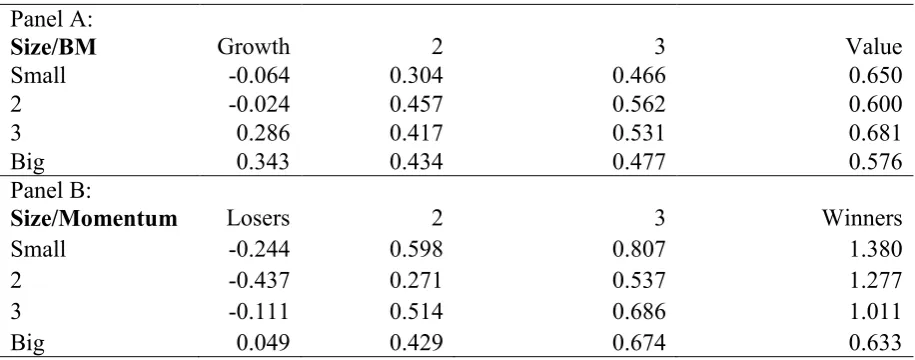
I use two groups of test assets, similar to Fama and French(2012), to examine the mean-variance efficiency of linear factor models in U.K. stock returns between July 1983 and December 2016. The first group is 16 portfolios of stocks sorted by size and book-to-market (BM) ratio. The second group is 16 portfolios of stocks sorted by size and momentum. The portfolios are value weighted buy and hold monthly returns. The portfolios include all U.K. stocks traded on the London Stock Exchange and smaller investment markets, which meet the criteria for inclusion. The stock return and market values come from the London Share Price Database (LSPD) provided by the London Business School, and book values come from Worldscope. I compute excess returns using the one-month U.K. Treasury Bill return from LSPD and Datastream. Full details on the construction of the test assets is available on request. Table 1 reports the average monthly excess returns of the size/BM portfolios (panel A) and size/momentum portfolios (panel B).
10
excess return than the Big portfolio. For the growth portfolios, the Big portfolio has a higher average excess return than the Small portfolio.
The size/momentum portfolios in panel B of Table 1 have a larger spread in average excess returns than the size/BM portfolios. The average excess returns range between -0.437% (2/Losers) and 1.380% (Small/Winners). There is a strong momentum effect as the Winners portfolio has a higher average excess return than the Losers portfolio across all size groups. The momentum effect is strongest in smaller companies. Compared to the size/BM portfolios, there is a stronger size effect in the size/momentum portfolios. Excluding the Losers portfolios, the Small portfolio has a higher mean excess return than the Big portfolio. The size effect is strongest in the Winners portfolios.
B) Factor Models
I focus on nine linear factor models in my study. Details of the construction of the factor models are available on request. The models include:
1. CAPM
This model is a single-factor model that uses the excess returns of the U.K. stock market index (Mkt) as the proxy for aggregate wealth.
2. Fama and French(1993) (FF)
The FF model is a three-factor model. The factors are the excess return on the market index and two zero-cost portfolios that capture the size (SMB) and value/growth (HML) effects in stock returns.
3. Carhart(1997)
11
This model is a five-factor model. The factors include the factors in the FF model and two zero-cost portfolios that capture the profitability (RMW) and investment growth (CMA) effects in stock returns. I refer to the SMB, HML, RMW, and CMA factors as combined spread factors using the notation of Fama and French(2017). The SMB factor constructed using the FF5 model is used across all models.
5. Fama and French(2017) (FF5s)
This model is a five-factor model. The factors are the market index, SMB, and the small ends of the combined spread factors of HML (HMLS), RMW (RMWS), and CMA (CMAS).
6. Fama and French(2017) (FF6)
This model is a six-factor model, which augments the FF5 model with the combined spread momentum (WML) factor.
7. Fama and French(2017) (FF6s)
This model is a six-factor model, which augments the FF5s model with the small end of the combined spread WML factor (WMLS).
8. Daniel et al(2018) (DHS)
12
This model is a six-factor model, which replaces the HML factor in the FF6 model with a more timely version (HMLT) of the value factor as in Asness and Frazzini(2013)9.
Table 2 reports summary statistics of the factor excess returns between July 1983 and December 2016. The summary statistics include the mean and standard deviation of monthly factor excess returns (%). The final column reports the t-statistic of the null hypothesis that the average excess returns on the factors equal zero.
Table 2 here
Table 2 shows that a number of the factors have significant positive average excess returns. The WMLS factor has the highest mean excess return at 1.218%, followed by the WML factor. This result confirms the strong momentum effect in U.K. stock returns, and the fact that momentum is stronger in smaller companies. The HML factor has a significant positive average excess return as does the HMLS factor. The higher average excess return on the HMLS factor confirms that the value effect is stronger in small companies. These patterns between the WML and WMLS factors and the HML and HMLS factors are consistent with Fama and French(2017) in U.S. stock returns. In contrast, the more timely version of the value (HMLT) factor has a lower average excess return than the HML factor and is statistically insignificant.
The SMB factor in Table 2 has a tiny average excess return. There is no significant profitability effect using the RMW factor. The average excess return on the RMW factor is
9 Barillas et al(2018) find that using the more timely version of the HML factor in the Fama
13
the second lowest across all factors. The average excess returns on the RMWS factor is significant at the 10% level. There is a strong investment effect, with significant mean excess returns on the CMA and CMAS factors. The two behavioural factors of Daniel et al(2018) also have significant mean excess returns. It is only for the CMA, WML, WMLS, CMAS and FIN factors that the t-statistics are larger than the critical t-value recommended by Harvey, Liu and Zhu(2016)10.
IV Empirical Results
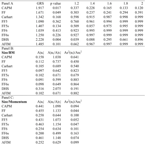
I begin my empirical tests by examining the mean-variance efficiency, using both the GRS test and the B-GRS test, for each of the nine linear factor models using both sets of test assets. Using the size/momentum portfolios as the test assets, both the GRS and B-GRS tests strongly reject the mean-variance efficiency of each factor model and so I only report the GRS and B-GRS tests for the size/BM portfolios. Table 3 reports the mean-variance efficiency tests using the size/BM portfolios (panel A) and summary metrics of performance based on the alpha11 in panels B (size/BM) and C (size/momentum) portfolios. The summary metrics include the mean absolute value of alpha (A|αi|), the mean absolute value of alpha divided by the mean absolute value of average excess return deviation from the market index (A|αi|/A|ri|), and the ratio of the mean squared standard error of alpha and the mean squared alpha (As2(αi)/Aαi2).
Table 3 here
10 Harvey et al(2016) find that prior empirical research have found 316 variables that are known
to be related to stock returns. To control for multiple testing issues, Harvey et al recommend the use of higher critical values of the t-statistic to judge statistical significance.
14
Panel A of Table 3 suggests that the rejection of mean-variance efficiency depends upon whether we use the GRS test or the B-GRS test. Using the GRS test, it is only the CAPM, FF, and DHS models that can be rejected at the 5% significance level. In contrast for the B-GRS test, there is little evidence against the mean-variance efficiency of the factor models. The exception to this result is for the DHS model, where the posterior probability is 0.039 when the prior maximum Sharpe ratio is 1.2. This difference in results between the GRS and B-GRS tests could be driven by the fact that under the alternative hypothesis the alphas in the GRS test are unbounded but are bounded in the GRS test.
Using the pricing error metrics to compare models, panel B of Table 3 shows that, the FF6 model has the best performance using the size/BM portfolios. The Carhart, FF5, FF5s, FF6s, and AFIM models all have similar performance using the A|αi| and A|αi|/A|ri| measures. Even although the mean-variance efficiency of these models cannot be rejected, each model still leaves a substantial proportion of the average excess returns unexplained. The minimum value of the A|αi|/A|ri| measure is 59.9%. Much of the variation in αi’s is due to sampling error. The poorest performing model is the DHS model, where all three pricing error metrics are noticeably poorer than the other models.
Using the size/momentum portfolios in panel C of Table 3, shows that the models that include a momentum factor, Carhart, FF6, FF6s, and AFIM models have the best performance using the A|αi| and A|αi|/A|ri| measures. The FF6s model is the best performing model among the models using these two metrics. The DHS model has again the poorest performance with the A|αi| and A|αi|/A|ri| measures. All of the models have low As2(αi)/Aαi2 measures, which suggests that the sampling error only explains a small proportion of the spread in alphas.
mean-15
variance efficiency of the factor models is similar to Fletcher(1994,2001) and Gregory et al(2013) in U.K. stock returns and Fama and French(2015,2016) in U.S. stock returns. Across the two sets of test assets, the pricing error metrics suggest that the best performing model is the FF6s model and the poorest performing model is the DHS model. The superior relative performance of the FF6s model is consistent with Fama and French(2017). The DHS model is at a disadvantage compared to the alternative multifactor models as the factors in these models are all formed using the same stock characteristics as used in forming the test assets.
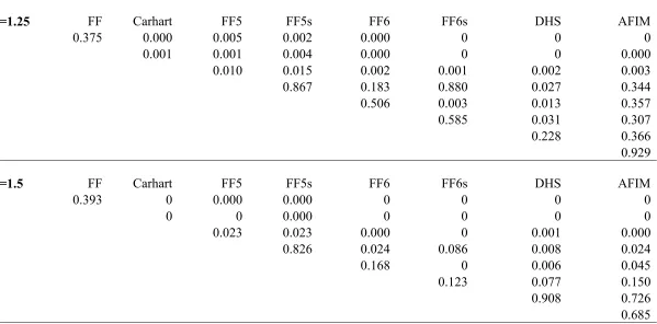
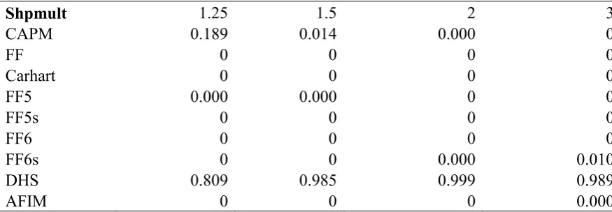
I next use the Bayesian approach to conduct pairwise model comparison tests and multiple model comparison tests between all nine factor models. The Bayesian pairwise model comparison tests are reported in Table 4 and the multiple model comparison tests are included in Table 5. The tables report the posterior probability of each model. The posterior probabilities in Table 4 are for the models in the rows and the corresponding probabilities for the models in the columns are one minus the posterior probabilities.
Table 4 here Table 5 here
16
relative performance of the Carhart model stands in sharp contrast to the pricing error metrics, where it is one of the best models.
Among the two five-factor models, the FF5 model has a considerable higher posterior probability than the FF5s model, suggesting better relative performance. This result differs from Fama and French(2017). At the higher prior maximum Sharpe ratio multiples of 2 and 3, both the FF5 and FF5s models significantly underperform the six-factor models. This result highlights the importance of the momentum factor. The DHS model also significantly outperforms the FF5 and FF5s models across all prior Sharpe ratio multiples.
Among the six-factor models, the FF6 model significantly underperforms the FF6s and AFIM models at the prior maximum Sharpe ratio multiples of 2 and 3. The good relative performance of the AFIM model, which uses the more timely HML factor, is consistent with Barillas et al(2018). The FF6s model significantly outperforms the AFIM model at the prior maximum Sharpe ratio multiples of 2 and 3. The DHS model significantly outperforms the FF6 model at prior Sharpe ratio multiples of 1.25 and 1.5. The DHS model performs less well relative to the FF6s model and significantly underperforms the FF6s model at prior maximum Sharpe ratio multiples of 1.5 and above.
17
The model comparison tests in Table 4 are based on pairwise model comparison tests. Table 5 shows that when conducting multiple model comparison tests, that the FF6s and AFIM models have a posterior probability close to zero. This result holds across all prior maximum Sharpe ratio multiples. This finding suggests that when conducting relative model comparison tests, it is important to take account of the excluded factors in all of the alternative models. The DHS model is the clear winner in Table 5. The posterior probability of the DHS model exceeds 0.98 when the prior maximum Sharpe ratio is 1.5 and above. This result is striking when considering the poor performance of the DHS model in the pricing error metric of the test assets in Table 3. It again highlights, as in Barillas and Shanken(2017), the importance of taking account of excluded factors when comparing factor models.
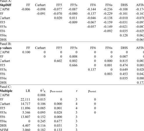
I repeat the model comparison tests but this time evaluate the models by the maximum squared Sharpe performance of Barillas et al(2018). Table 6 reports the pairwise (panels A and B) model comparison tests, and panel C reports the multiple model comparison tests using the maximum squared Sharpe performance. Panel A presents the difference in the bias-adjusted maximum squared Sharpe performance (ShpDiff)12 between every pair of models and panel B are the corresponding p values of the equality of the squared Sharpe performance between every pair of models. Where the ShpDiff measure is negative (positive), the squared Sharpe performance of the model in the row is lower (higher) than the model in the column. Panel C includes the LR test of Wolak(1987,1989) of the multiple non-nested model
12 It is well known that the sample ML estimate of θ2K has an upward bias (Ferson and
18
comparison tests and corresponding p value (pnon-nested)13. The r column is the number of alternative non-nested models, and θ2K is the bias-adjusted squared Sharpe performance of each model. The final column includes the p value of the multiple nested model comparison tests. The test statistics are corrected for heteroscedasticity.
Table 6 here
Panels A and B of Table 6 show that as with the Bayesian model comparison tests, the CAPM and FF models perform poorly relative to the alternative multifactor models. Both models provide a significant lower squared Sharpe performance than all the alternative models and are strongly rejected in the multiple model comparison tests. The Carhart model performs better in Table 6 compared to the Bayesian tests and yields a similar maximum squared Sharpe performance to the FF5, FF5s, and DHS models. However the Carhart model significantly underperforms the three six-factor models and is strongly rejected in the multiple model comparison tests. In contrast to the Bayesian tests, the FF5 and FF5s model yield a similar squared Sharpe performance, which is more consistent with Fama and French(2017). Likewise both models yield a similar squared Sharpe performance to the DHS model. However both the FF5 and FF5s models significantly underperform the FF6s and AFIM models. Both models are likewise rejected in the multiple model comparison tests.
Among the three six-factor models, the FF6 model provides a significant lower squared Sharpe performance than the FF6s and AFIM models. The FF6 model is also rejected in the multiple model comparison tests. The FF6s model has a significant higher squared Sharpe
13 Using a bootstrap approach to estimate the p values of the LR test are similar to those reported
19
performance than the AFIM model at the 10% significance level. The FF6s model also provides a significant higher squared Sharpe measure than the DHS model. However in the multiple non-nested model comparison tests using either the FF6s or AFIM models as the benchmark, we cannot reject the null hypothesis that each model performs as well as the alternative models in terms of squared Sharpe performance. In contrast to the Bayesian multiple model comparison tests, the DHS model no longer delivers superior performance as we can reject the null hypothesis that the DHS model performs as well as the alternative non-nested models.
The model comparison tests in Table 6 provide an alternative perspective on relative model performance to the Bayesian tests in Tables 4 and 5. The FF6s model performs well using both approaches. In contrast the DHS model performs well in the Bayesian tests but not in the classical tests due to the smaller bias-adjusted maximum squared Sharpe performance. The Bayesian approach focuses on the marginal likelihood of the model given the underlying prior belief of the alphas, whereas the classical test focuses directly on the maximum squared Sharpe performance. Combining the evidence from both model comparison approaches, would suggest that the FF6s model has the best relative performance among the set of models considered.
V Conclusion
This paper uses the Bayesian and classical approaches of Barillas and Shanken(2018) and Barillas et al(2018) to conduct model comparison tests of nine linear factor models in U.K. stock returns. The study likewise tests the mean-variance efficiency of each model using the classical Gibbons et al(1989) test and the Bayesian approach of Barillas and Shanken. There are four main findings from my study.
20
the size/BM portfolios as the test assets, the B-GRS test provides a more favourable picture of model performance than the GRS test. The rejection of the mean-variance efficiency of the linear factor models in U.K. stock returns is consistent with earlier studies such as Fletcher(1994,2001), Gregory et al(2013) among others and in U.S. stock returns as Fama and French(2015,2016). Using the pricing error metrics of the test assets to compare models, the FF6s model has the best performance. Most of the factor models perform reasonably well in the size/BM portfolios. Models that include the momentum factor (Carhart, FF6, FF6s, and AFIM) have the best performance in the size/momentum portfolios. The DHS model has the poorest performance using the pricing error metrics of the test assets. The DHS model is at an inherent disadvantage to the alternative multifactor models as they are formed using the same set of stock characteristics involved in forming the test assets.
Second, in the Bayesian pairwise model comparison tests the FF6s model has the best performance. The AFIM and DHS models also perform well. The striking result is that some of the best performing models in the pricing error metrics of the test assets such as the Carhart model perform poorly in the pairwise model comparison tests but the converse is true of the DHS model. This finding is consistent with Barillas and Shanken(2017) that evaluating models by pricing error metrics of the test assets can give different results to looking at the pricing of excluded factors.
21
Fourth, using the classical model comparison tests of Barillas et al(2018) shows that the FF6s and AFIM models have the best performance using the maximum squared Sharpe performance. The FF6s model is able to significantly outperform all the alternative factor models at the 10% significance level. In contrast, the DHS model performs less well and is only able to significantly outperform the CAPM and FF models. This finding suggests that the Bayesian and classical approaches to model comparison can give different results and each approach evaluates the models from a different perspective.
22
Table 1 Summary Statistics of Test Assets Panel A:
Size/BM Growth 2 3 Value
Small -0.064 0.304 0.466 0.650
2 -0.024 0.457 0.562 0.600
3 0.286 0.417 0.531 0.681
Big 0.343 0.434 0.477 0.576
Panel B:
Size/Momentum Losers 2 3 Winners
Small -0.244 0.598 0.807 1.380
2 -0.437 0.271 0.537 1.277
3 -0.111 0.514 0.686 1.011
Big 0.049 0.429 0.674 0.633
23
Table 2 Summary Statistics of Factors
Factor Mean Standard Deviation t-statistic
Market 0.434 4.185 2.071
SMB 0.015 2.945 0.10
HML 0.300 2.552 2.351
RMW 0.145 2.018 1.44
CMA 0.411 1.896 4.341
WML 0.907 3.789 4.801
HMLS 0.391 3.039 2.581
RMWS 0.210 2.278 1.852
CMAS 0.482 2.002 4.831
WMLS 1.218 3.664 6.661
FIN 0.426 1.755 4.871
PEAD 0.254 2.224 2.281
HMLT 0.202 3.209 1.26
1 Significant at 5% 2 Significant at 10%
24
Table 3 Tests of Mean-Variance Efficiency of Factor Models
Panel A GRS p value 1.2 1.4 1.6 1.8 2
CAPM 1.917 0.017 0.337 0.228 0.165 0.133 0.120
FF 1.671 0.049 0.303 0.237 0.241 0.294 0.391
Carhart 1.342 0.168 0.598 0.915 0.987 0.998 0.999
FF5 1.090 0.362 0.760 0.961 0.994 0.999 0.999
FF5s 1.407 0.134 0.509 0.857 0.975 0.995 0.999
FF6 1.039 0.413 0.923 0.995 0.999 0.999 0.999
FF6s 1.250 0.226 0.927 0.997 0.999 0.999 0.999
DHS 2.228 0.004 0.039 0.088 0.295 0.661 0.896
AFIM 1.485 0.101 0.662 0.967 0.997 0.999 0.999
Panel B:
Size/BM A|αi| A|αi|/A|ri| As2(αi)/Aαi2
CAPM 0.158 1.038 0.641
FF 0.112 0.737 0.450
Carhart 0.105 0.689 0.540
FF5 0.097 0.642 0.823
FF5s 0.102 0.671 0.679
FF6 0.091 0.599 0.883
FF6s 0.098 0.649 0.864
DHS 0.316 2.075 0.191
AFIM 0.102 0.671 0.882
Panel C:
Size/Momentum A|αi| A|αi|/A|ri| As2(αi)/Aαi2
CAPM 0.441 1.098 0.094
FF 0.455 1.133 0.044
Carhart 0.258 0.644 0.100
FF5 0.431 1.073 0.052
FF5s 0.463 1.154 0.047
FF6 0.254 0.634 0.101
FF6s 0.200 0.499 0.163
DHS 0.461 1.148 0.074
AFIM 0.252 0.629 0.099
25
Table 4 Bayesian Pairwise Model Comparison Tests Panel A:
Shpmult=1.25 FF Carhart FF5 FF5s FF6 FF6s DHS AFIM
CAPM 0.375 0.000 0.005 0.002 0.000 0 0 0
FF 0.001 0.001 0.004 0.000 0 0 0.000
Carhart 0.010 0.015 0.002 0.001 0.002 0.003
FF5 0.867 0.183 0.880 0.027 0.344
FF5s 0.506 0.003 0.013 0.357
FF6 0.585 0.031 0.307
FF6s 0.228 0.366
DHS 0.929
Panel B:
Shpmult=1.5 FF Carhart FF5 FF5s FF6 FF6s DHS AFIM
CAPM 0.393 0 0.000 0.000 0 0 0 0
FF 0 0 0.000 0 0 0 0
Carhart 0.023 0.023 0.000 0 0.001 0.000
FF5 0.826 0.024 0.086 0.008 0.024
FF5s 0.168 0 0.006 0.045
FF6 0.123 0.077 0.150
FF6s 0.908 0.726
26
Panel C:
Shpmult=2 FF Carhart FF5 FF5s FF6 FF6s DHS AFIM
CAPM 0.485 0 0 0 0 0 0 0
FF 0 0 0 0 0 0 0
Carhart 0.058 0.040 0.000 0 0.000 0
FF5 0.763 0.002 0.000 0.001 0.000
FF5s 0.024 0 0.001 0.001
FF6 0.005 0.184 0.055
FF6s 0.998 0.959
DHS 0.209
Panel D:
Shpmult=3 FF Carhart FF5 FF5s FF6 FF6s DHS AFIM
CAPM 0.655 0 0 0 0 0 0 0
FF 0 0 0 0 0 0 0
Carhart 0.135 0.074 0 0 0.000 0
FF5 0.696 0.000 0 0.000 0
FF5s 0.003 0 0.000 0.000
FF6 0.000 0.259 0.022
FF6s 0.999 0.995
DHS 0.058
27
Table 5 Bayesian Multiple Model Comparison Tests
Shpmult 1.25 1.5 2 3
CAPM 0.189 0.014 0.000 0
FF 0 0 0 0
Carhart 0 0 0 0
FF5 0.000 0.000 0 0
FF5s 0 0 0 0
FF6 0 0 0 0
FF6s 0 0 0.000 0.010
DHS 0.809 0.985 0.999 0.989
AFIM 0 0 0 0.000
28
Table 6 Model Comparison Tests using the Squared Sharpe Performance Panel A:
ShpDiff FF Carhart FF5 FF5s FF6 FF6s DHS AFIM
CAPM -0.006 -0.098 -0.077 -0.087 -0.144 -0.236 -0.108 -0.174
FF -0.091 -0.070 -0.080 -0.137 -0.229 -0.101 -0.167
Carhart 0.020 0.011 -0.046 -0.138 -0.010 -0.076
FF5 -0.009 -0.067 -0.159 -0.031 -0.097
FF5s -0.057 -0.149 -0.021 -0.087
FF6 -0.092 0.035 -0.029
FF6s 0.128 0.062
DHS -0.065
Panel B:
p values FF Carhart FF5 FF5s FF6 FF6s DHS AFIM
CAPM 0.100 0 0 0 0 0 0 0
FF 0 0 0.008 0 0 0.007 0
Carhart 0.602 0.802 0 0.000 0.815 0.003
FF5 0.666 0 0.001 0.474 0.001
FF5s 0.137 0 0.649 0.020
FF6 0.003 0.453 0.042
FF6s 0.035 0.080
DHS 0.173
Panel C:
Multiple LR θ 2
K pnon-nested r pnested
CAPM 0.008
FF 22.111 0.015 0 3 0
Carhart 14.717 0.106 0.000 4 0
FF5 11.896 0.085 0.001 4 0
FF5s 5.346 0.095 0.028 3 0
FF6 13.807 0.152 0.000 3
FF6s 0 0.245 0.677 3
DHS 4.407 0.116 0.031 3
AFIM 3.060 0.182 0.133 3
29
References
Asness, C. and A. Frazzini, 2013, The devil in HML’s details, Journal of Portfolio
Management, 39, 49-68.
Asness, C.S., Frazzini, A., Israel, R. and T. Moskowitz, 2015, Fact, fiction, and value investing,
Journal of Portfolio Management, 42, 34-52.
Barillas, F., Kan, R., Robotti, C. and J. Shanken, 2018, Model comparison with Sharpe ratios,
Working Paper, University of Toronto.
Barillas, F. and J. Shanken, 2017, Which alpha?, Review of Financial Studies, 30,1316-1388. Barillas, F. and J. Shanken, 2018, Comparing asset pricing models, Journal of Finance, forthcoming.
Carhart, M. M., 1997, Persistence in mutual fund performance. Journal of Finance, 52, 57-82. Chretien, S. and M. Kammoun, 2017, Mutual fund performance evaluation and best clienteles,
Journal of Financial and Quantitative Analysis, 52, 1577-1604.
Cochrane, J.H. and J.Saa-Requejo, 2000, Beyond arbitrage: Good-deal asset price bounds in incomplete markets, Journal of Political Economy, 108, 79-119.
Daniel, K., Hirshleifer, D. and L. Sun, 2018, Short- and long-horizon behavioural factors, Working
Paper, Columbia University.
Davies, J.R., Fletcher, J. and A. Marshall, 2015, Testing index-based models in U.K. stock returns, Review of Quantitative Finance and Accounting, 45, 337-362.
Fama, E.F. and K.R. French, 1993, Common risk factors in the returns on stocks and bonds.
Journal of Financial Economics 33, 3-56.
Fama, E.F. and K.R. French, 2012, Size, value, and momentum in international stock returns,
Journal of Financial Economics, 105, 457-472.
Fama, E.F. and K.R. French, 2015, A five-factor asset pricing model, Journal of Financial
30
Fama, E.F. and K.R. French, 2016, Dissecting anomalies with a five-factor model, Review of
Financial Studies, 29, 69-103.
Fama, E.F., and K.R. French, 2017, Choosing factors, Working Paper, University of Chicago. Ferson, W.E. and A.F. Siegel, 2003, Stochastic discount factor bounds with conditioning information, Review of Financial Studies, 16, 567-595.
Ferson, W.E. and A.F. Siegel, 2009, Testing portfolio efficiency with conditioning information,
Review of Financial Studies, 22, 2735-2758.
Ferson, W.E. and A. F. Siegel, 2015, Optimal orthogonal portfolios with conditioning information, C.F. Lee, Editor, Handbook of Financial Econometrics, Springer Science and Business Media, New York.
Fletcher, J., 1994, The mean-variance efficiency of benchmark portfolios: UK evidence,
Journal of Banking and Finance, 18, 673-685.
Fletcher, J., 2001, An examination of alternative factor models in UK stock returns, Review of
Quantitative Finance and Accounting, 16, 117-130.
Gibbons, M.R., Ross, S.A. and J. Shanken, 1989, A test of the efficiency of a given portfolio,
Econometrica, 57,1121-1152.
Gospodinov, N., Kan, R. and C. Robotti, 2013, Chi-squared tests for evaluation and comparison of asset pricing models, Journal of Econometrics, 173, 108-125.
Gregory, A., Tharyan, R. and A. Christidis, 2013, Constructing and testing alternative versions of the Fama-French and Carhart models in the UK, Journal of Business Finance and Accounting, 40, 172-214.
Grinblatt, M. and S. Titman, 1983, Factor pricing in a finite economy, Journal of Financial
Economics, 12, 497-507.
31
Grinblatt, M. and K. Saxene, 2017, When factors don’t span their basis portfolios, Journal of
Financial and Quantitative Analysis, forthcoming.
Hansen, L.P. and R. Jagannathan, 1997, Assessing specification errors in stochastic discount factor models, Journal of Finance 52, 591-607.
Harvey, C.R., 2017, The scientific outlook in financial economics, Journal of Finance, 72, 1399-1440.
Harvey, C.R., Liu, Y. and H. Zhu, 2016, … and the cross-section of expected returns, Review of
Financial Studies, 29, 5-68.
Harvey, C.R. and Y. Liu, 2018, Lucky factors, Working Paper, Duke University.
Harvey, C.R. and G. Zhou, 1990, Bayesian inference in asset pricing tests, Journal of Financial
Economics, 26, 221-254.
Hou, K., Xue, C. and L. Zhang, 2015, Digesting anomalies: An investment approach, Review of
Financial Studies, 28, 650-705.
Hou, K., Xue, C. and L. Zhang, 2017, Replicating anomalies, Working Paper, Ohio State University.
Huang, D. and G. Zhou, 2017, Upper bounds on return predictability, Journal of Financial and
Quantitative Analysis, 52, 401-425.
Kan, R. and C. Robotti, 2008, Specification tests of asset pricing models using excess returns,
Journal of Empirical Finance, 15, 816-838.
Kan, R., Robotti, C. and J. Shanken, 2013, Pricing model performance and the two-pass cross-sectional regression methodology, Journal of Finance, 68, 2617-2649.
MacKinlay, A.C. 1995, Multifactor models do not explain deviations from the capital asset pricing model, Journal of Financial Economics, 38, 3-28.
32
McCulloch, R.E. and P.E. Rossi, 1991, A Bayesian approach to testing the arbitrage pricing theory, Journal of Econometrics, 49, 141-168.
Michou, M. and H. Zhou, 2016, On the information content of new asset pricing factors in the
UK, Working Paper, University of Edinburgh.
Pastor, L. and R.F. Stambaugh, 2000, Comparing asset pricing models: An investment perspective, Journal of Financial Economics, 56, 335-381.
Roll, R., 1977, A critique of the asset pricing theory’s test; Part I: On past and potential testability of the theory, Journal of Financial Economics, 4, 129-176.
Shanken, J., 1987, A Bayesian approach to testing portfolio efficiency, Journal of Financial
Economics, 19, 195-216.
Sharpe, W.F., 1966, Mutual fund performance, Journal of Business 39, 119-138.
Stambaugh, R.F. and Y. Yuan, 2017, Mispricing factors, Review of Financial Studies, 30, 1270-1315.
Wolak, F.A., 1987, An exact test for multiple inequality and equality constraints in the linear regression model, Journal of the American Statistical Association, 82, 782–793.
Wolak, F.A., 1989, Testing inequality constraints in linear econometric models, Journal of