City, University of London Institutional Repository
Citation:
Ben-Gad, M. (2017). The Optimal Taxation of Asset Income when Government Consumption is Endogenous: Theory, Estimation and Welfare. Economic Inquiry, 55(4), pp. 1689-1711. doi: 10.1111/ecin.12463This is the accepted version of the paper.
This version of the publication may differ from the final published
version.
Permanent repository link:
http://openaccess.city.ac.uk/16928/Link to published version:
http://dx.doi.org/10.1111/ecin.12463Copyright and reuse: City Research Online aims to make research
outputs of City, University of London available to a wider audience.
Copyright and Moral Rights remain with the author(s) and/or copyright
holders. URLs from City Research Online may be freely distributed and
linked to.
City Research Online: http://openaccess.city.ac.uk/ publications@city.ac.uk
The Optimal Taxation of Asset Income when Government
Consumption is Endogenous: Theory, Estimation and Welfare
Michael Ben-Gad∗ Department of Economics City, University of London
Northampton Square London EC1V 0HB, UK
December 2016
Abstract
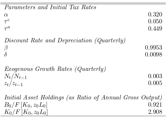
This paper derives the Ramsey optimal policy for taxing asset income in a model where government expenditure is a function of net output or the inputs that produce it. Extending Judd (1999), I demonstrate that the canonical result that the optimal tax on capital income is zero in the medium to long term is a special case of a more general model. Employing a vector error correction model to estimate the relationship between government consumption and net output or the factor inputs that generate it for the United States between 1948Q1 to 2015Q4, I demonstrate that this special case is empirically implausible, and show how a cointegrating vector can be used to determine the optimal tax schedule. I simulate a version of the model using the empirical estimates to measure the welfare implications of changing the tax rate on asset income, and contrast these results with those generated in a version of the model where government consumption is purely exogenous. The shifting pattern of welfare measurements confirms the theoretical results. I calculate that the prevailing effective tax rate on net asset income in the US between 1970 and 2014 averaged 0.449. Hence abolishing the tax completely does generate welfare improvements, though only by the equivalent of between 1.103 and 1.616% percent permanent increase in consumption—well under half the implied welfare benefit when the endogeneity of the government consumption is ignored. The maximum welfare improvement from shifting part of the burden of tax from capital to labor is the equivalent of a permanent increase in consumption of between only 1.491 and 1.858%, and is attained when the tax rate on asset income is lowered to between 0.148 and 0.186. Allowing the tax rate to vary over time raises the maximum welfare benefit to 1.865%. All the results are very robust to a wide range of elasticities of labor supply.
JEL classification: E62, H21, H50
Keywords: Fiscal Policy; Optimal Taxation; Vector Error Correction Model
∗mbengad@city.ac.uk. I would like to thank Giovanni Melina, Joseph Pearlman and Gustavo Sanchez as well as
1
Introduction
If governments must fund their activities by taxing income, on which sources of income should
the burden fall? In this paper I consider a general optimal growth model, one in which there
is a direct link between either aggregate net output or the factor inputs that produce it, and
the share of output allocated to government consumption. In such an economy the canonical
results of zero taxation of capital income no longer hold. I demonstrate that for an empirically
plausible specification of the link between government consumption and either net output or
factor inputs, there is a simple relationship that can be employed to determine the optimal rate
of tax on asset income and estimate a range of appropriate rates for the United States. Finally,
I measure the welfare implications of shifting the burden of taxation between asset income and
labor earnings. I demonstrate that the optimal tax rate on asset income is indeed positive, but
that given the prevailing rates of taxation in the United States, the maximal welfare benefit that
can be obtained from adopting an optimal policy is much smaller than what usually emerges
when government consumption expenditure is assumed to be exogenously determined.
Atkinson and Stiglitz (1976) demonstrated how the tax on interest income depends on the
complementarity or substitutability between consumption and leisure in a representative agent’s
instantaneous utility function. Additive separability between the two, implies the optimal tax
rate on interest is zero. Chamley (1981) was the first to calculate the excess burden associated
with the taxation of income from endogenously determined capital in a complete general
equi-librium setting. Judd (1985) and Chamley (1986) extended this work and demonstrated that in
standard optimal growth models, models where capital and consumption converge to a steady
state, the optimal long-run policy sets the tax rate on income from capital to zero. Judd (1999)
showed that for a wider class of dynamic models, particularly models that do not necessarily
converge to a single steady state or balanced growth path, optimal policy still entails setting
the tax rate on capital income to at least an average of zero over time.
In Chamley (1981), (1986), and Judd (1985), taxes are imposed to finance a fixed amount of
government expenditure. By contrast, in Judd’s (1999) more general formulation, government
expenditure is a public good that enters the utility function of the representative agent. In none
of this work is government expenditure directly related to economic output or its production.
In Section 2, I adopt Judd’s (1999) approach to determining optimal fiscal policy in models that
may not necessarily possess a single steady state or balanced growth path, but I distinguish
between public spending on transfer payments and government consumption. The latter is first,
a general function of factor inputs, and then more specifically a function of the economic output
the factors generate. Zero taxation of asset income does not emerge here as an optimal policy
except as a special case. Instead, if we assume that government consumption and domestic
output, net of depreciation, are related to each other in a particular way—one that can be
easily estimated as a cointegrating vector—a simple formula for the optimal tax rate on asset
1950 1960 1970 1980 1990 2000 2010 250
500 1000 2500 5000 10 000 20 000 50 000
Billions
of
2009
US$
H
Logarithmic
Scale
L
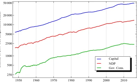
[image:4.595.81.525.86.351.2]Gov. Cons. NDP Capital
Figure 1: Capital, net domestic product and government consumption, quarterly in the United
States, deflated using the NDP deflator, 1948Q1 to 2015Q4, natural logarithmic scale. Data
Source: Federal Reserve Economic Data, Federal Reserve Bank of St. Louis; U.S. Department
of Commerce: Bureau of Economic Analysis seasonally adjusted variables and Fernald “A
Quar-terly, Utilization-Adjusted Series on TFP.” Federal Reserve Bank of San Francisco: Capital,
An-nual Net Assets [K1TTOTL1ES000] interpolated using quarterly changes in private capital from
Fernald; Net Domestic Product [A362RC1Q027SBEA]; Government Consumption Expenditures
[A955RC1Q027SBEA]; Deflator [A362RG3Q086SBEA]. http://research.stlouisfed.org/fred2/
and http://www.frbsf.org/economic-research/indicators-data/total-factor-productivity-tfp/.
Consider the behaviour of government consumption expenditure, capital and net domestic
product in the United States from 1948 onward in Figure 1. Throughout this work I use
nominal data deflated by the net domestic product deflator—the focus here is on the financing
of government consumption expenditure, so real volume measures of government outputs would
generate a distorted picture of how much net output is devoted to government consumption
or what portion of the capital stock is devoted to its production. Whereas the rise in the
amount spent on transfer payments has caused total government expenditure to grow at a
faster pace than the economy as a whole, the portion of net domestic output devoted to direct
government spending on goods and services closely tracks overall net domestic product—an
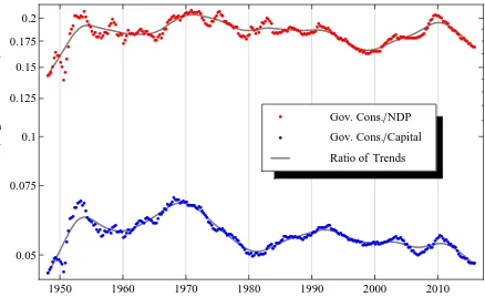
impression reinforced if we consider in Figure 2, either the evolution of the share of government
As I demonstrate in the first part of Section 3, both are integrated series and there exists
a cointegrating relationship between them that can be captured by estimating a vector error
correction model.
In contrast to Chamley (1981), (1986), and Judd (1985), (1999), in the model in Section 2
more capital accumulation leads not only to higher output but to higher government
consump-tion as well. Hence in the absence of a tax on the income it generates, the amount of capital the
economy will accumulate will be innefficiently high. As it this underlying relationship between
government consumption and capital that determines the optimal rate of taxation, in the second
part of Section 3, I estimate the cointegrating relationship between government consumption
and factor inputs. Forecasts generated by these very same vector error correction models can
then be used to provide estimates of the long-run optimal tax rate on asset income.
Finally in Section 4, I incorporate the estimates from Section 3 into the calibration of an
optimal growth model with elastic labor supply and measure the welfare implications of shifting
the tax burden from income derived from assets to labor earnings. As has been demonstrated
in previous studies by Coleman (2000), Domeij and Heathcote (2004), Eerola and M¨a¨att¨anen
(2013), ˙Imrohoro˘glu (1998), Laitner (1995) and Lucas (1990), the prevailing rate of tax on
asset income is sufficiently high in the United States that in the context of a representative
agent framework, eliminating it completely and shifting the burden to labor income has the
potential to generate a substantial positive welfare benefit. Qualitatively this effect is retained,
but if government consumption flows are directly related to economic activity (production or
capital accumulation) the magnitude of the benefit will be significantly smaller. Indeed, rather
than eliminating the tax completely, a more modest shift, one that lowers the effective tax
rate on net asset income from its recent long-run average of 0.449 to between 0.148 and 0.186
(depending on the model specification chosen), generates the greatest (though still relatively
modest) improvement in welfare, equivalent to a permanent increase in consumption of between
1.491% and 1.858%. These numbers can be improved upon, though only to a very small extent,
if the tax rate is permitted to shift slightly over time in the vicinity of this range.
As far back as Adolph Wagner (1883) and Henry Carter Adams (1898), Economists, have
postulated a close relationship between the amount of government expenditure and the overall
size of the economy. Indeed, a sizable empirical literature has developed to examine and explain
this relationship, starting with the seminal work by Peacock and Wiseman (1961) for the United
Kingdom. Yet rarely is this feature incorporated into models studying optimal fiscal policy.
Taken together, the theoretical and empirical results of this work suggest that failure to consider
the relationship between the share of net output devoted to government activity that taxes help
finance and the overall size and productive capacity of the economy in general has the potential
to skew our conclusions regarding the best allocation of the tax burden across the different
input factors.
••••
••••
••
••
••
••••••••••••••••••••••••••••••••••
••••••••••••••••••••••••••••
•••••••••••••••••••••••••••••••••••••••••••••
••••••••••••••••••••••••••••••••••••••••••••••••••••••••••••••••••••••••
•••••••••••••••••••••••••••••••••••••••••••••••
••••••••••••••••••••••
••••••••••
•••••••••••• ••
••••••• ••••
••••••
••••••••••••••••••••••••• ••••••••••••••••••
•••••••••••••••••••••••••••• •••••••••••
•••••••••••••
••••••••••••••••••••••••
••••••••••••••••••••••••••••••••••••••••••••••••••
•••••••••••••••••••••••••••••••
•••••••••••••••••••••••••••••••••••• •••••
1950 1960 1970 1980 1990 2000 2010
0.05 0.075 0.1 0.125 0.15 0.175 0.2
Fraction
of
NDP
H
Logarithmic
Scale
L
Ratio of Trends
• Gov. Cons.Capital
[image:6.595.82.520.84.352.2]• Gov. Cons.NDP
Figure 2: The ratios of government consumption expenditure to net domestic product or capital
stock in the United States, combined with the ratios of each of their trend components from
Hodrick Prescott Filters (the value of the penalty parameter is set to λ=1600), 1948Q1 to
2015Q4.
When I left graduate school, in 1963, I believed that the single most desirable
change in the U.S. tax structure would be the taxation of capital gains as ordinary
income. I now believe that neither capital gains nor any of the income from capital
should be taxed at all.
Yet the continued development of dynamic general equilibrium models that endogenise the
supply of capital has not settled the argument regarding the efficacy of taxing the income it
generates. Aiyagari (1995), Correia (1996), Reis (2011) and others, all find that under conditions
of uninsurable idiosyncratic risk, asymmetric information, or the inability of governments to
tax some factor inputs, Ramsey optimal policies will include some taxation of capital income.
This work implies that even in the absence of uncertainty, incomplete markets, or asymmetric
information, imposing some of the burden of funding government expenditure on capital income
can be an economically efficient policy that maximises the welfare of a representative agent,
provided there is a functional relationship between government consumption, the capital stock
and the overall size of the economy. Indeed, rather than setting the tax rate on asset income to
zero, a welfare optimising policy for the United States would imply the near equalising of net
imposed on asset income and earnings will stem from the burden of debt service, which should
fall solely on the latter.
2
Theory: Ramsey Optimal Policy
2.1 The Representative Household’s Problem
We begin by reformulating Judd’s (1999) optimal taxation argument in discrete time and also
alter his model to make government consumption a function of either factor inputs or the net
output they together produce. Assume an economy in which all participants are members of
households that share the instantaneous utility function u:R2+ → R, which maps preferences
over consumption and labor, and a discount factor β ∈ (0,1). Utility is strictly increasing in
consumption, and strictly decreasing in labor. I normalize the size of the initial population to
N0=1, and a representative household chooses its consumptionctand labor inputltto maximise
its infinite horizon discounted utility:
max
c,l
∞
∑
t=0
βtNtu[ct, lt] (P.1)
subject to
Nt+1at+1 =Nt( ¯wtlt+ (1 + ¯rt)at−p¯tct+ht) (1)
where at represents assets (both bonds and capital); ht represents net government transfer
payments; ¯wt, ¯rt and ¯pt represent the time t after tax wage rate, after-tax rate of return on
asset holding and after-tax price of consumption; the size of the population isNt, and the net
rate of population growth between timetand t+ 1 isNt+1/Nt−1.
Differentiating the optimization problem P.1 with respect to ct,ct+1,lt and at+1 yields the
first order conditions:
uc[ct, lt]−λtp¯t= 0, (2)
ul[ct, lt] +λtw¯t= 0, (3)
−λt+βλt+1(1 + ¯rt+1) = 0, (4)
where uc[ct, lt] > 0 and ul[ct, lt] < 0 are the marginal utilities of consumption and labor,
and λt is a current value costate variable that expresses the marginal utility derived by the
representative household from a positive increment to asset wealth.1
2.2 The Social Planner’s Problem
Output in this economy is produced by combining aggregate capitalKt and aggregate effective
labor ztLt, which is the aggregate labor input itselfLt=Ntlt multiplied by labor augmenting
technology zt. I denote the production function as F :R2+ → R+. Capital depreciates at the
1
constant rateδ ≥0, and so net domestic product, defined as output net of capital depreciation
isYt≡F[Kt, ztLt]−δKt. We assume competitive firms maximise profits, so that pre-tax factor
returnsrt andwt equal their marginal products. I also assume the production technologyF is
homogenous of degree 1, so that in equilibrium:
rt=F1[Kt, ztLt]−δ, (5)
wt=ztF2[Kt, ztLt]. (6)
The government raises revenue in each periodt by selling one period bonds Bt+1, collecting a
tax on labor earningsτtl= 1−w¯t
wt, collecting a taxτ
a
t = 1−rr¯tt levied on income from the returns
generated by either of the two assets, physical capital or the bonds themselves, and collecting
an ad valorem tax τtc= p¯t
pt −1 on consumption ct. In this real economy we normalise the
pre-tax price of the consumption good pt to one. Together all these revenues finance government
consumption, which here is confined to that portion of government activity represented on
the expenditure side of the national accounts which is not designated as investment, finance
an exogenous stream of transfer payments, or redeem the interest and principal of all the
outstanding debt incurred in the period prior. In contrast to most of the optimal tax literature,
where government consumption is fixed, or Judd (1999), where it enters the utility function of
both the representative agent and the social planner, here I assume that like output, it is a
function of both aggregate inputs, G:R2+→R+. The government’s budget constraint is:
Bt+1=G[Kt, ztLt] +Ht−τtlwtLt−τtart(Kt+Bt) + (1 +rt)Bt−τtcCt, (7)
where Bt is the aggregate stock of government bonds at the beginning of time t, Ct = Ntct
represents aggregate consumption flows during this period, andHt=Nthtrepresents aggregate
government transfer payments.
Now consider the Ramsey problem of a policy maker who chooses per-capita consumption
ct, leisure lt, the after-tax price of consumer goods ¯pt, and after-tax factor returns ¯rt and ¯wt
which maximise the representative households’ discounted utility:
max
c,l,¯r,w,¯p¯
∞
∑
t=0
βtNtu[ct, lt] (P.2)
subject to the incentive compatibility constraints (2) to (4), the feasibility condition:
Kt+1 =F[Kt, ztLt]−G[Kt, ztLt] + (1−δ)Kt−Ct, (8)
and assuming the aggregate production function F is homogenous of degree one, the
govern-ment’s budget constraint (7), which can be reformulated as:
Bt+1 = ¯rt(Kt+Bt) + ¯wtLt+δKt−F[Kt, ztLt] +G[Kt, ztLt]−(¯pt−1)Ct+Bt+Ht. (9)
Budget constraints (8) and (9), when combined imply (1) after it is aggregated. I assume
limt−>∞|bt|<∞and also:
¯
¯
wt≥0, (11)
¯
pt≥0. (12)
Differentiating the social planner’s optimization problem P.2 with respect to ¯pt, ¯wt, ¯rt,λt, and
the per-capita values ct,lt,kt+1, and bt+1 yields the first order conditions:
uc[ct, lt]−ϕtk+ϕctucc[ct, lt] +ϕltucl[ct, lt]−µt(¯pt−1) = 0, (13)
ul[ct, lt] +ztϕkt(F2[Kt, ztLt]−G2[Kt, ztLt]) +µt( ¯wt−ztF2[Kt, ztLt] +ztG2[Kt, ztLt])
+ϕctucl[ct, lt] +ϕltull[ct, lt] = 0, (14)
−µt
ct
pt−
ϕctλt+νtp= 0, (15)
µtlt+λtϕlt+νtw = 0, (16)
ϕλt−1Nt−1λt+µt(Kt+Bt) +Ntνtr = 0, (17)
Nt−1ϕλt−1(1 + ¯rt)−Nt
(
βϕλt +ϕctp¯t−ϕltw¯t
)
= 0, (18)
−ϕkt +βϕkt+1(F1[Kt+1, zt+1Lt+1]−G1[Kt+1, zt+1Lt+1] + 1−δ)
+βµt+1(¯rt+δ−F1[Kt+1, zt+1Lt+1] +G1[Kt+1, zt+1Lt+1]) = 0, (19)
−µt+βµt+1(1 + ¯rt+1) = 0. (20)
where ϕct, ϕlt, ϕλt, µt, ϕkt, νtr, νtw, and ν
p
t are the costates variables associated with (2), (3),
(4), (8), (9), (10), (11) and (12). Straub and Werning (2015) demonstrate that under certain
conditions, a social planner will prefer policies such as setting ¯rt= 0,∀t, that have the effect of
driving both the stock of capital and consumption to zero in the long-run, rather than interior
solutions. In what follows, I restrict my attention to interior solutions to (13) to (20) and
assume thatνtr =νtp =νtw = 0.
In the absence of any tax distortions, the marginal value at time tof an increment of capital
for the representative household, λt > 0 is equal to its marginal value for the social planner,
ϕkt >0. Similarly, in a model in which taxes are not distortionary and do not generate excess
burdens, Ricardian equivalence prevails, and the neutrality of public debt held in household
asset portfolios implies that µt = 0. Otherwise, as is the case here, servicing any increase in
the public debt burden entails deadweight losses so that µt < 0. Following Judd (1999), I
define Λt≡ p¯1tϕ
k
t−µt
λt , which is a measure of the social value of an increment to physical capital
when the value of private assets (comprising both capital and public debt) is held constant,
and the reciprocal of ¯pt corrects for the distorting effect of ad-valoreum taxes paid on private
consumption. Again, in a model without distortionary taxation, ¯pt= 1, ϕkt =λt and µt= 0 so
therefore Λt= 1.
Judd (1999) assumes that government expenditure enters the utility function as a way to
ensure that the value of Λt>0. It is, however, possible to achieve the same result by placing a
Lemma 1. A sufficient condition that ensures that Λt>0 for allct>0, kt >0 and lt>0, is
ul[ct, lt] +lull[ct, lt] +cucl[ct, lt]≤0 and zt(F2[Kt, ztLt]−G2[Kt, ztLt])>0.
Proof. Solving (14) for ϕkt, subtractingµt, substituting the interior solutions for (15) and (16)
forϕct andϕlt (withνtp=νtw= 0), and replacing ¯wt using (3) yields:
ϕkt −µt= −
uc[ct, lt]ul[ct, lt] +µt(ul[ct, lt] +ltull[ct, lt] +ctucl[ct, lt])
uc[ct, lt]zt(F2[Kt, ztLt]−G2[Kt, ztLt])
. (21)
From the assumptions thatuc[ct, lt]>0 andul[ct, lt]<0,ϕkt −µt>0 iful[ct, lt] +lull[ct, lt] +
cucl[ct, lt] ≤ 0 and zt(F2[Kt, ztLt]−G2[Kt, ztLt]) > 0. Finally from (2) λt > 0 and hence
Λt>0.
After substituting (4), (19) and (20), the value of Λt evolves according to:
Λt+1
Λt
= p¯t
¯
pt+1
1 + ¯rt+1
1 +F1[Kt+1, zt+1Lt+1]−G1[Kt+1, zt+1Lt+1]−δ
. (22)
The numerator in the right-hand side of (22), 1 + ¯rt+1 when multiplied by the price ratio p¯pt¯+1t ,
is the cost agents in this economy face when they shift a unit of consumption between period
t and t+ 1. The denominator reflects the cost of this shift in terms of production, which here
includes the portion of extra output lost to additional government consumption. Iterating (22)
from period tbackwards:
Λt
Λ0
= p¯0
¯
pt t
∏
i=1
1 + ¯ri
1 +F1[Ki, ziLi]−G1[Ki, ziLi]−δ
. (23)
Assume that along a balanced growth path the ad valoreum tax rate on consumption is
constant so that ¯pt = ¯p0. Comparing the growth rates for the costate variables µt and λt
in (4) and (20), we know the ratio µt/λt is always constant. If this economy converges to a
steady state or a balanced growth path, once convergence is complete, the ratioϕkt/λt will have
converged to a constant value as well. Hence for an economy that has converged, a solution
to the social planner’s problem implies the value Λt is a constant and (23) implies that the
sequence {1 + ¯ri}ti=1 must be set to ensure the ratio Λt/Λ0 is equal to one.
Theorem 1. Suppose an economy converges to a steady state or balanced growth path, then
assuming an interior solution for (13) to (20), the long-run optimal policy is to set r¯ equal
to limt→∞F1[Kt, ztLt]−G1[Kt, ztLt]−δ. The social planner accomplishes this by setting the
long-run tax rateτa equal to limt→∞G1[Kt, ztlt]/(F1[Kt, ztlt]−δ).
Proof. Follows from Λt/Λ0 = 1 in (23).
Indeed, notice how the same trajectory of Λt/Λ0 can be generated by choosing either the
sequence {1 + ¯ri}ti=1 or the ratio
¯
p0
¯
pt. The social planner has more policy instruments than
Corollary 1. The availability of a consumption tax is not necessary to ensure a Ramsey second
best allocation associated with the optimization problem P.2.
Proof. From (4) and (20) we know that µt+1
λt+1 =
µt
λt ∀t. Combining (17) with (18) and inserting
the values of Kt+1 and Bt+1 from (8) and (9) yields:
µt
λt
( ¯wtlt−ct)−ϕct+ϕltw¯t= 0.
Combining this with (16) while assuming an interior solution so that νtw = 0 yields:
ϕct=−µt
λt
ct,
which replicates (15) as long asνtp = 0.Since (15) is implied by the other first order conditions,
for any interior solution the availability to the social planner of a consumption tax does not
alter the result in Theorem 1.
In what follows, we assume that ¯pt is always constant. A number of special cases emerge
from Theorem 1, depending on how the functionGis specified. For example, ifG1[Kt, ztLt] = 0
so that government consumption is not a function of the capital stock, we recover the canonical
Chamley-Judd result of zero taxation on asset income as the long-run optimising policy. This
is the case even if G2[Kt, ztLt] ̸= 0, and government consumption is still a function of the
amount of effective labor employed in production. Alternatively if G1[Kt, ztLt]̸= 0, then
en-dogenous government expenditure creates a wedge between the net marginal product of capital
F1[K, zL]−δ, and corresponding interest rate r, that confronts individuals in this economy,
and the full marginal product of capital F1[K, zL]−G1[K, zL]−δ, as it is perceived by the
social planner. The tax rate imposed on assetsτa serves to compensate for this disparity.
For example, if G1[Kt, ztLt] < 0, then any policy that encourages capital accumulation
depresses the amount of output diverted to government consumption, and the optimal policy
is to subsidise capital income by setting ¯r to be less than r and τa < 0. If G[Kt, ztLt] =
gKt−β(ztLt)1+β, then even in a model with exponential steady state growth, government
ex-penditure as a share of GDP still converges to a strictly positive amount, and yet the optimal
tax is still negative. Finally, if G1[Kt, ztLt]>0 then the optimal tax rate is positive.
In an economy in which government expenditure is exogenously determined, the long-run
supply curve for capital is infinitely elastic at a given interest rate. This is why the distortions
associated with policies that lower the after-tax rate of return dominate those that directly
affect labor supply. By contrast, for the type of economies specified in Theorem 1, a change
in the tax rate on asset income alters not just the amount of capital available to produce the
consumption good, but indirectly affects the overall amount of government consumption, which
here does not have the usual lump-sum quality. Instead, government consumption is itself a
type of distortion that asset taxation serves to mitigate. This remains the case even if the
Consider the case of the power function G[Kt, ztLt] = g(F[Kt, ztLt]−δKt)γ, and g > 0
and γ >0. Suppose the values of zt and Nt converge to constants, and the economy converges
to a stationary steady state. Government consumption converges to a positive share of net
output and the optimal long-run tax rate on asset income is γg(F[Kt, ztLt]−δKt)γ−1.2 By
contrast, if we assume zt and/or Nt are growing, we must constrain the value of γ to be less
than or equal to one, to ensure that government consumption does not ultimately exceed net
output. If there exists a balanced growth path and γ = 1, government consumption converges
to a positive share of outputg, and the long-run optimal policy will be one where the tax rate
is positive so that τa = g. If, however, γ < 1, and the aggregate economy is growing, then
limt→∞g(F[Kt, ztLt]−δKt)γ−1= 0, which means we recover the Chamley-Judd optimal
long-run policy of setting ¯r=F1[K, zL]−δ and τa = 0 in the limit—though as I will demonstrate
below, until the economy converges, the optimal policy may be very different.
Theorem 1 applies to economies that have converged to a balanced growth path. What
then should be the policy if the economy does not converge to a balanced growth path but is
characterized by cycles, or, alternatively, convergence is achieved only over a very long time
horizon. Can we say anything about optimal policy in the interim?
First, the results in Theorem 1 and the after tax rate of return as t→ ∞do not depend on
the distorting properties of the other taxes, on the evolution of lump-sum transfers or whether
they are positive or negative. Indeed it remains valid even if in the initial period the social
planner is able to set ¯r0 = 0 and confiscate all asset income in the initial period. In that case
an optimising social planner will deploy the additional revenue from what amounts to an initial
lump sum tax towards reducing the distortionary impact of wage taxation. To see this, assume
the utility function is not a function of labor hours supplied in the market, but depends on
consumption alone, and that Ht is a policy variable. Labor taxation and transfers are now
completely interchangable and for these two policy instruments Ricardian equivalence prevail—
the shadow price of government debt µt is equal to zero. Yet the reasoning behind Theorem 1
remains intact. The social planner will set the value of ¯r = limt→∞F1[Kt, ztLt]−G1[Kt, ztLt]−δ
to ensure that ϕkt = λt. More often, when analysing optimal factor taxation, we exclude the
option of resorting to lump-sum taxation as an alternative source of revenue. Suppose, in what
follows, we constrainHt to be equal to zero.
The challenge here is that regardless of what the long-run optimum policy is, during the
initial period, the social planner might want to set the value ¯r0 very low to exploit the time-zero
inelasticity of capital supply and replicate the now missing option of imposing a lump sum tax.
It is this reasoning that gives rise to the “bang-bang” pattern of optimal taxation described by
Chamley (1986). This is why, even though the more a sequence of tax rates on asset income
causes the value of Λt to deviate from one, the more it distorts the economy and generates
welfare losses, it is not possible to pin down the initial value of Λ0 or assume it equals one. Yet
2Ben-Gad (2003) analyses long-run optimal fiscal policy along a balanced growth path in the context of a
if we assume that an optimal programme will seek to minimise distortions beyond an initial
period of high taxation, subsequent values of Λt must be bounded below and above over time:
Λ∞<Λ<Λ∞. Setting the bounds and rewriting the inequalities in logarithms yields:
ln ( Λ0 Λ∞ ) ≤ t ∑ i=1 ln (
1 +F1[Ki, ziLi]−G1[Ki, ziLi]−δ
1 + ¯ri
) ≤ln ( Λ0 Λ∞ ) , (24)
which implies that as the value of Λt in (23) evolves over a sufficiently long period of time,
it must on average be equal to one and the average distortion measured as deviations from
Λt = 1 approaches zero in the limit. Extending Judd (1999), this implies that for all t1 ≥0,
any long-run constant value of ¯r must satisfy:
lim
t2→∞
1
t2
t∑1+t2
i=t1
ln (
1 +F1[Ki, ziLi]−G1[Ki, ziLi]−δ
1 + ¯r
)
= 0, (25)
which in turn implies that if the social planner must choose a particular constant tax rate, then:
Theorem 2. Assume there exists an interior solution for (13) to (20), for any t1 ≥ 0, if the
value ofr¯ is fixed, then the long-run optimal policy is to set it to satisfy (25).
Theorem 2 generalises Theorem 1 to economies that may not converge to balanced growth
paths or steady states. For example, if the dynamic behaviour of the economy is characterized
by permanent cycles, and ¯r is to be fixed to any value, it will be optimally so, if on average it
equalsF1[Kt, ztLt]−G1[Kt, ztLt]−δ and the long-run tax rateτaon asset income is set to the
average value of G1[Kt, ztLt]/(F1[Kt, ztLt]−δ). Yet this leaves the question of what is the
best policy if the policy maker is not necessarily constrained to choose fixed values for ¯rt and
τta?
To avoid the issue of time inconsistency, assume a policy maker commits to an infinite
sequence of ¯rt that need not be constant. An infinite number of different sequences satisfy the
boundary conditions in (24) and hence also satisfy
lim
t2→∞
1
t2
t∑1+t2
i=t1
ln (
1 +F1[Ki, ziLi]−G1[Ki, ziLi]−δ
1 + ¯ri
)
= 0. (26)
Yet only by committing to a policy of setting ¯ri equal to F1[Ki, ziLi]−G1[Ki, ziLi]−δ and
tax ratesτia equal to G1[Ki, ziLi]/(F1[Ki, ziLi]−δ) in each period does a policy maker both
satisfy (25) and minimise deviations from Λt= 1.
Theorem 3. For a sufficiently large value of t1 ≥0, an optimal tax policy for asset income is
such that the values of r¯i are set equal to F1[Ki, ziLi]−G1[Ki, ziLi]−δ.
Proof. By satisfying (26) such a policy simultaneously minimizes deviations from Λt= 1 over
time and satisfies the boundary conditions in (24). It generalizes Theorem 6 in Judd (1999) as
well as Theorem 2 above to the case where the policy maker is not constrained to set tax rates
Theorem 3 can be implemented by setting the sequence of tax rates τia equal to
G1[Ki, ziLi]/(F1[Ki, ziLi]−δ). There is however an obvious limitation to the practical
ap-plicability of the Theorem—the difficulty in determining the appropriate size of the initial t1
periods during which the social planner may choose to set the tax rate on asset income very
high to exploit the short-term inelasticity in the supply of capital.3 Yet regardless of the length
oft1, we can utilize the intuition that underlies Theorem 3 to generate a useful conjecture about
how different tax policies are likely to compare. Once again we focus on the power function.
Conjecture 1. Suppose government consumption is a power function of net domestic product,
G[Kt, ztLt] =g(F[Kt, ztLt]−δKt)γ.Then a policy of setting the sequence of tax ratesτia equal
to γG[Kt, ztLt]/(F[Kt, ztLt]−δKt), which equals γg(F[Kt, ztLt]−δKt)γ−1 for all periods
t≥0, weakly dominates a policy of fixingτa to any fixed value. Furthermore, ifγ = 1, then the
policy of fixing τa=g strictly dominates the policy of fixingτa to any value τa̸=g.
Setting aside the possibility of employing a “bang-bang” optimal control policy through
period t1, Conjecture 1 predicts how the welfare effects of different tax policies, if implemented
immediately, are likely to compare, and not merely over the long-run, if the relationship between
government consumption and net output takes a very particular form, the power function.
More generally, one possible interpretation of the function G[Kt, ztLt], one that
general-izes beyond the context of the strictly theoretical models considered in this section, is that
it expresses a long-run equilibrating relationship between government consumption and either
factor inputs or the economic output, net of depreciation, they generate. Provided government
consumption and net output are integratedI(1) processes, perhaps because they share a trend
driven by labor augmenting technology and/or population growth as in the model above, the
specific case of the power function is easily estimated, as it corresponds in its logarithmic form to
the cointegrating relationship in Johansen’s Vector Error Correction Model (VECM). If capital
and effective labor are I(1) as well, it is also possible to replace net output with factor inputs
and establish the cointegrating relationship between capital and government expenditure that
is fundamental to the theory. In the next section I use the VECM to estimate both types of
relationship, and then in Section 4 I incorporate these estimates into the calibration of a model
designed to numerically evaluate the main implications of Conjecture 1.
3
Estimation: Error Correction Models for Government
Con-sumption
3.1 Government Consumption and Net Output
We start by examining the properties of government consumptionGt, and net domestic product
in the United StatesYt, using quarterly data from the first quarter of 1948 to the fourth quarter
3
of 2014. In Table 1, neither the augmented Dickey-Fuller, the Dickey–Fuller test with GLS
detrending, the Elliott-Rothenberg-Stock point-optimal test, Phillips-Perron test or Ng and
Perron’s MZα, MZt, MSB and MPttests cannot reject the null hypothesis of a unit root at the
1% critical level when applied to the levels of each series, but all reject the existence of unit
roots at the 1% level when applied to the series’ first differences. Perron and Vogelsang’s or
Zivot and Andrew’s Dickey-Fuller tests which each accounts for breaks in both the trend or
constant (in levels) or the constant (in differences) generate the same pattern, and fail to find
evidence of spurious unit root behavior. Similarly, the KPSS test rejects the null hypothesis of
stationarity in the levels of each of the two series at the 1% level, but cannot reject the null
hypothesis when applied to differences, as long as the test includes a deterministic time trend
(which in each case is statistically significant).
For the ratio of the two series (log differences) in the last two columns, the augmented
Dickey-Fuller and Phillips-Perron test each rejects the existence of a unit root at the 1% critical level.
Accounting for break points weakens but does not contradict these results and the
Kwiatkowski-Phillips-Schmidt-Shin (KPSS) cannot reject the null hypothesis of stationarity of the ratio at
the 10% critical value (the deterministic time trend in KPSSt is not statistically significant).4
However the the Dickey–Fuller test with GLS detrending, the Elliott-Rothenberg-Stock
point-optimal test, Ng and Perron’s MZα, MZt, and MPt cannot reject the null hypothesis of a unit
root even at the 10% critical level. Together, these contradictory results could imply that if the
two series are cointegrated and characterized by the exponential relationship in Section 2 the
value of γ might fall somewhere in the vicinity of one.
To test for cointegration, I begin by estimating an unrestricted VAR for the two time series.
The optimal lag lengthpfor the estimated VAR indicated by the Aikake’s information criterion,
Akaike’s final prediction error (FPE) and the likelihood ratio (LR) is q = 4, but Schwarz’s
Bayesian information criterion (SBIC) and the Hannan and Quinn information criterion (HQIC)
indicate, as is often the case, a more parsimonious optimal lag length, q = 2, which is what I
choose to use. If government consumption and net domestic product do indeed share a common
stochastic trend, the largest eigenvalue of the system must be equal to one, and to guarantee
stability all the others must be (in modulus) less than one. The largest eigenvalue here is .997,
the next highest is .911, and the two complex eigenvalues 0.341 + .030ithe fall well within the
unit circle.
To determine the cointegrating vector itself, I estimate the Vector Error Correction Model
4A Quandt-Andrews breakpoint test performed on an AR(1) estimation of the log ratio cannot reject the null
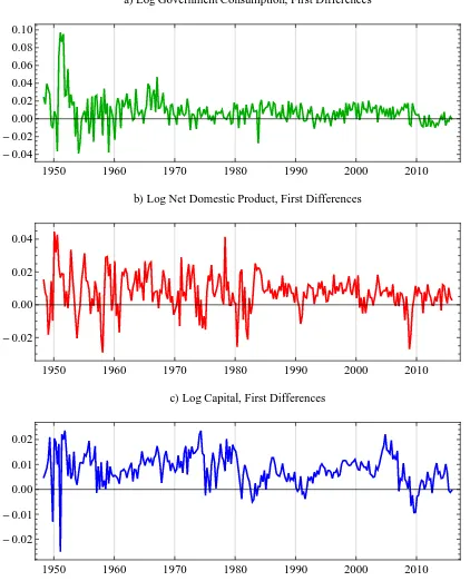
1950 1960 1970 1980 1990 2000 2010
-0.04 -0.02
0.00 0.02 0.04 0.06 0.08 0.10
aLLog Government Consumption, First Differences
1950 1960 1970 1980 1990 2000 2010
-0.02
0.00 0.02 0.04
bLLog Net Domestic Product, First Differences
1950 1960 1970 1980 1990 2000 2010
-0.02 -0.01
0.00 0.01 0.02
[image:16.595.88.510.123.645.2]cLLog Capital, First Differences
Figure 3: Log differences of government consumption, net domestic product and log capital,
quarterly in the United States, seasonally adjusted annual rate deflated by the NDP deflator,
Method Gov. Consumption Net Domestic Product Gov. Cons./NDP
Level First Diff. Level First Diff. Level
ADF -2.678 -5.895∗∗∗ -1.678 -11.028∗∗∗ -4.328∗∗∗
DF-GLS -0.736 -3.540∗∗∗ -0.970 -6.543∗∗∗ -1.613
PT-GLS 46.307 0.948∗∗∗ 26.203 0.319∗∗∗ 17.658
PP -2.916 -12.085∗∗∗ -1.509 -11.066∗∗∗ -3.849∗∗
MZα -2.916 -22.231∗∗∗ -3.232 -66.434∗∗∗ -6.096
MZt -0.828 -3.296∗∗∗ -1.008 -5.749∗∗∗ -1.658
MSB 0.377 0.148∗∗∗ 0.312 0.087∗∗∗ 0.272
MPt 31.315 1.236∗∗∗ 23.092 0.402∗∗∗ 14.900
DF-PV -4.352 -7.099∗∗∗ -3.595 -11.392∗∗∗ -4.811
DF-ZA -4.369 -8.207∗∗∗ -3.743 -8.576∗∗∗ -5.508∗∗
KPSSnt 2.137††† 0.564†† 2.181††† 0.387† 0.214
[image:17.595.74.545.70.257.2]KPSSt 0.356††† 0.071 0.391††† 0.027 0.189††
Table 1: Nominal data deflated by NDP deflator, in natural logarithms. ADF is the augmented
Dickey–Fuller test. DF-GLS is the Dickey–Fuller test with GLS detrending. PT-GLS is the
Elliott-Rothenberg-Stock point-optimal test statistic. PP is the Phillips-Perron test. MZa,
MZt, MSB, and MPt are the modified tests in Ng and Perron (2001). DF-PV and DF-ZA
are the Perron and Vogelsang and Zivot and Andrews unit root tests with intercept and trend
breaks. All these tests are conducted with a constant term and trend for levels and ratios, and
a constant term only for first differences. Finally, KPSSnt is the
Kwiatkowski-Phillips-Schmidt-Shin test without deterministic time trend while KPSSt includes the trend. ∗ Reject the null
hypothesis of a unit root at the 10% confidence level. ∗∗Reject the null hypothesis of a unit root
at the 5% confidence level. ∗∗∗ Reject the null hypothesis of a unit root at the 1% confidence
level. † Reject the null hypothesis of stationarity at the 10% confidence level. †† Reject the
null hypothesis of stationarity at the 5% confidence level, ††† Reject the null hypothesis of
stationarity at the 1% confidence level.
(VECM): (
∆ lnGt
∆ lnYt
) = ( θG θY )
(lnGt−1−γlnYt−1−lng) (27)
+
q
∑
i=1
(
ζGG(i) ζGY (i)
ζY G(i) ζY Y (i)
) (
∆ lnGt−i
∆ lnYt−i
) + ( ηG ηY ) + ( εG,t εY,t ) ,
whereθGandθY represent the spead of adjustment, the vector (1, γ)′ represents the normalised
cointegrating vector and g is a constant. If γ = 1, then the long-run relationship between
government consumption and net domestic product is a fixed proportion, represented by the
constant term g. Together γ and g correspond to the parameters in the power function that
expresses the long-run relationship between government consumption and net output in Section
2.
Define the 2×2 matrix Φ≡
(
θG
θY
) (
1 γ ). From Johansen’s trace and maximum
Rank Eigen. Trace p-Value Max-Eigen. p-Value
0 1
0.092 0.013
29.402 3.416
<0.001
0.065
25.986 3.416
0.001 0.065
Table 2: Johansen’s trace and maximum eigenvalue tests along with information criteria for the
rank of the matrix αβ for government consumption and net domestic product.
confidence level but do not reject the hypothesis of one cointegrating vector (rather than full
rank). Together this implies that (1, γ)′ represents a valid cointegrating vector that, together
with the estimated value of g, represents the long-run relationship between government
con-sumption and net domestic product.5
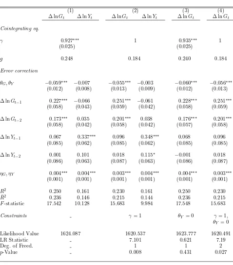
Given the contradictory results the different tests for the stationarity of the ratio between
government consumption and net output yield, it is not surprising that the estimate ofγ = 0.927
in the unrestricted vector error correction model (27) in column (1) of Table 3 is close to, yet
still more than two and a half standard deviations from one. Hence we can reject the restriction
ofγ to one in column (2) with ap-value of 0.008. The estimate ofθG is statistically significant
but the estimate ofθY is not, implying that net output is weakly exogenous.That is consistent
with the theoretical model in Section 2 which implies that government consumption is directly
determined by the values of the parametersg and γ and the level of economic activity. Hence
we cannot reject the restriction that the value of θY is zero in column (3), in which case the
value ofγ rises slightly to 0.935. However we can reject, at least a the 5% level, the imposition
of both constraints in column (4).
So what do the results in Table 3 tell us about optimal tax policy? First, if we do impose
the constraint γ = 1, the optimal long-run tax on asset income is simply equal to the value of
g or 0.184 which is also the long-run average share of government consumption in net output
between 1948 and 2015. By contrast, if γ < 1, as our estimates imply, and the size of the
economy continues to grow in the future, either because of per-capita output growth or the
increasing size of the work force, the share devoted to government consumption declines as its
growth fails to completely keep pace with that of net output. As mentioned in Section 2, such
scale effects mean the limiting optimal tax rate as t → ∞ coincides with the Chamley-Judd
rate of zero.
Yet immediately setting the rate of tax to zero would not minimise distortions as described
in Theorem 3. Even if we believe the estimated power relationship is stable over long periods of
time, decades or even centuries may pass before the value of γg(F[Kt, ztLt]−δKt)γ−1 decays
by any significant amount.
5
(1) (2) (3) (4)
∆ lnGt ∆ lnYt ∆ lnGt ∆ lnYt ∆ lnGt ∆ lnGt
Cointegrating eq.
γ 0.927∗∗∗ 1 0.935∗∗∗ 1
(0.025) (0.025)
g 0.248 0.184 0.240 0.184
Error correction
θG, θY −0.059∗∗∗ −0.007 −0.055∗∗∗ −0.003 −0.060∗∗∗ −0.056∗∗∗
(0.012) (0.008) (0.013) (0.009) (0.012) (0.013)
∆ lnGt−1 0.227∗∗∗ −0.066 0.251∗∗∗ −0.061 0.228∗∗∗ 0.251∗∗∗
(0.058) (0.043) (0.059) (0.042) (0.058) (0.059)
∆ lnGt−2 0.173∗∗∗ 0.035 0.201∗∗∗ 0.038 0.176∗∗∗ 0.201∗∗∗
(0.058) (0.042) (0.058) (0.042) (0.057) (0.058)
∆ lnYt−1 0.067 0.337∗∗∗ 0.096 0.348∗∗∗ 0.068 0.096
(0.085) (0.062) (0.085) (0.062) (0.085) (0.085)
∆ lnYt−2 0.001 0.101 0.018 0.115∗ −0.001 0.018
(0.086) (0.063) (0.087) (0.063) (0.086) (0.087)
ηG, ηY 0.004∗∗∗ 0.004∗∗∗ 0.003∗∗∗ 0.004∗∗∗ 0.004∗∗∗ 0.003∗∗∗
(0.001) (0.001) (0.001) (0.001) (0.001) (0.001)
R2 0.250 0.161 0.230 0.161 0.250 0.230
¯
R2 0.236 0.146 0.215 0.144 0.236 0.215
F-statistic 17.542 10.128 15.683 9.984 17.548 15.683
Constraints γ = 1 θY = 0 γ = 1,
θY = 0
Likelihood Value 1624.087 1620.537 1623.777 1620.491
LR Statistic 7.101 0.621 7.19
Deg. of Freed. 1 1 2
[image:19.595.78.556.111.656.2]p-Value 0.008 0.431 0.027
Table 3: Estimated Vector Error Correction Model for US data on government consumption
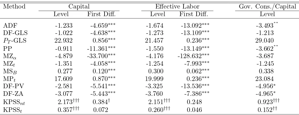
Method Capital Effective Labor Gov. Cons./Capital
Level First Diff. Level First Diff. Level
ADF -1.233 -4.659∗∗∗ -1.674 -13.092∗∗∗ -3.493∗∗
DF-GLS -1.022 -4.638∗∗∗ -1.273 -13.109∗∗∗ -1.213
PT-GLS 22.932 0.856∗∗∗ 21.457 0.236∗∗∗ 29.040
PP -0.911 -11.361∗∗∗ -1.550 -13.149∗∗∗ -3.662∗∗
MZα -4.879 -33.700∗∗∗ -4.176 -128.632∗∗∗ -3.687
MZt -1.351 -4.058∗∗∗ -1.254 -7.993∗∗∗ -1.245
MSB 0.277 0.120∗∗∗ 0.300 0.062∗∗∗ 0.338
MPt 17.609 0.870∗∗∗ 19.999 0.236∗∗∗ 23.084
DF-PV -2.581 -5.541∗∗∗ -3.325 -13.536∗∗∗ -4.956∗
DF-ZA -3.077 -5.443∗∗∗ -3.760 -7.386∗∗∗ -4.965∗
KPSSnt 2.173††† 0.384† 2.151††† 0.248 0.923†††
[image:20.595.73.565.70.259.2]KPSSt 0.357††† 0.072 0.260††† 0.046 0.152††
Table 4: Nominal data deflated by NDP deflator, in natural logarithms. For description of the
tests, see caption in Table 1
3.2 Government Consumption and Factor Inputs
It is the underlying connection between government consumption and capital that generates
the policy prescriptions in Theorems 1 through 3. Is there in fact a cointegrating relationship
between government consumption and the two aggregate factor inputs, and in particular to
capital? First, to generate data for the total capital stock Kt at a quarterly frequency in
Figures 1 and 2, I using the quarterly rates of change in private capital estimated by Fernald
(2014) to interpolate quarterly estimates of total fixed assets between the available end of year
figures. Then using nominal gross domestic product, and assuming a constant returns to scale
Cobb-Douglas production function, I employ simple growth accounting to generate a series that
corresponds to effective labor,ztLt. When applied to each factor input, the unit roots tests in
Table 4 reveal a pattern similar to those in Table 1—alone each series isI(1) but tests on the
ratio of government consumption to capital yield results that are as contradictory as those for
the ratio of government consumption to net output.
When applied to estimates of unrestricted vector autoregressions with the logarithm of
government expenditure lnGt, the logarithm of aggregate capital lnKt, and the logarithm of
effective labor ln (ztLt), SBIC once again suggests the optimal number of lags is equal to 2.
The eigenvalues of the system are stable, the largest equal to 0.998, and the next highest 0.971.
Both Johansen’s trace and maximum eigenvalue tests for cointegration in Table 5 support the
Rank Eigen. Trace p-Value Max-Eigen. p-Value 0 1 2 0.078 0.032 0.008 32.846 10.817 2.106 0.022 0.223 0.147 22.029 8.710 2.106 0.037 0.311 0.147
Table 5: Johansen’s trace and maximum eigenvalue tests along with information criteria for the
rank of the matrix αβ for government consumption, aggregate capital and effective labor.
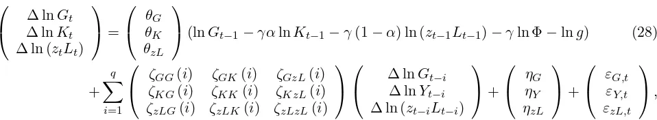
The counterpart here to (27) is:
∆ ln∆ lnGKtt
∆ ln (ztLt)
=
θθKG
θzL
(lnGt−1−γαlnKt−1−γ(1−α) ln (zt−1Lt−1)−γln Φ−lng) (28)
+
q
∑
i=1
ζζGGKG((ii)) ζζKKGK((ii)) ζζKzLGzL((ii))
ζzLG(i) ζzLK(i) ζzLzL(i)
∆ ln∆ lnGYtt−−ii
∆ ln (zt−iLt−i)
+
ηηGY
ηzL
+
εεG,tY,t
εzL,t
,
where Φ relates to the rate of depreciation, or more precisely represents the ratio between net
domestic product Ytand gross domestic product ˜Yt =Yt+δKt. I treat this as a constant and
set its value to its long-run average between 1948 to 2015, Φ=0.889.6 Given that the series
for effective labor was constructed using a constant returns to scale production technology, the
value of the estimated coefficients on lnKt−1 and ln (zt−1Lt−1) in (28) must by construction
equal γ, which allows me to isolate the value of g from the estimate of the constant in the
cointegrating vector.
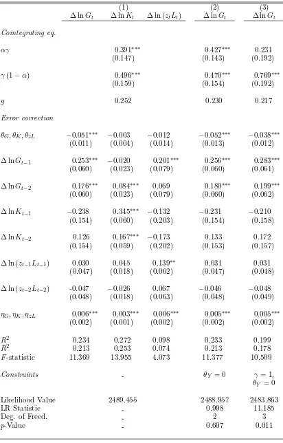
The unrestricted estimates of the model in the columns labeled (1) in Table 6 imply values
of α= 0.441, g= 0.252 andγ = 0.887—the latter two estimates are not significantly different
from the corresponding estimates in Table 3.7 The constraint that the sum of the values of the
two coefficients in (28) are equal to one can be rejected at the 1% level. However, once again
the estimates this time ofθKandθzLsuggest that both aggregate capital and effective labor are
weakly exogenous, and this is confirmed in the column labeled (2) where thep-value associated
with the constraint is 0.607. In this specification the estimates imply: α = 0.476, g = 0.230
and γ = 0.897. The column labeled (3) includes estimates where the constraintsγ = 1 as well
as θK = 0 and θzL = 0. Here the p-value associated with the constraint is only 0.011, so we
can once again reject this additional restriction. Again the estimates in both Tables 3 and 6
confirm what the tests for stationarity of the ratios in Tables 1 and 4 suggest—that the value
of γ is close to, yet statistically speaking, significantly less than one.
6Estimating Φ as the constant term in the cointegrating vector for Y
t−1 and ˜Yt−1 yields nearly identical
results.
7
(1) (2) (3)
∆ lnGt ∆ lnKt ∆ ln (ztLt) ∆ lnGt ∆ lnGt
Cointegrating eq.
αγ 0.391∗∗∗ 0.427∗∗∗ 0.231
(0.147) (0.143) (0.192)
γ(1−α) 0.496∗∗∗ 0.470∗∗∗ 0.769∗∗∗
(0.159) (0.154) (0.192)
g 0.252 0.230 0.217
Error correction
θG, θK, θzL −0.051∗∗∗ −0.003 −0.012 −0.052∗∗∗ −0.038∗∗∗
(0.011) (0.004) (0.014) (0.013) (0.012)
∆ lnGt−1 0.253∗∗∗ −0.020 0.201∗∗∗ 0.256∗∗∗ 0.283∗∗∗
(0.060) (0.023) (0.079) (0.060) (0.061)
∆ lnGt−2 0.176∗∗∗ 0.084∗∗∗ 0.069 0.180∗∗∗ 0.199∗∗∗
(0.060) (0.023) (0.079) (0.060) (0.062)
∆ lnKt−1 −0.238 0.345∗∗∗ −0.132 −0.231 −0.210
(0.154) (0.060) (0.203) (0.154) (0.158)
∆ lnKt−2 0.126 0.167∗∗∗ −0.173 0.133 0.172
(0.154) (0.059) (0.202) (0.153) (0.157)
∆ ln (zt−1Lt−1) 0.030 0.045 0.139∗∗ 0.031 0.031
(0.047) (0.018) (0.062) (0.047) (0.048)
∆ ln (zt−2Lt−2) -0.047 −0.026 0.067 −0.046 −0.048
(0.048) (0.018) (0.063) (0.048) (0.049)
ηG, ηK, ηzL 0.006∗∗∗ 0.003∗∗∗ 0.006∗∗∗ 0.005∗∗∗ 0.005∗∗∗
(0.002) (0.001) (0.002) (0.002) (0.002)
R2 0.234 0.272 0.098 0.233 0.199
¯
R2 0.213 0.253 0.074 0.213 0.178
F-statistic 11.369 13.955 4.073 11.377 10.509
Constraints θY = 0 γ = 1,
θY = 0
Likelihood Value 2489.455 2488.957 2483.863
LR Statistic 0.998 11.185
Deg. of Freed. 2 3
[image:22.595.93.505.70.714.2]p-Value 0.607 0.011
Table 6: Estimated Vector Error Correction Model for US data on government consumption,
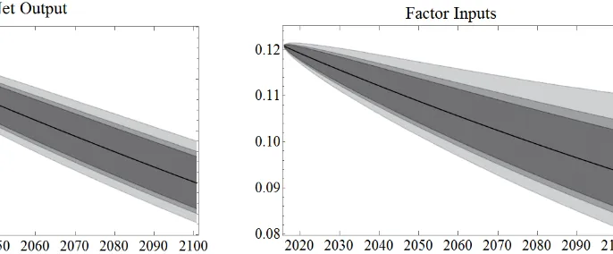
Figure 4: Forecasts for the value of γGt/Yt from 2016Q1 to 2100Q4 derived from the vector
error correction model with net output in (27) and estimated in column (3) of Table 3, and the
model with factor outputs in (28) estimated in column (2) of Table 6. Grey shading indicates
confidence bands of 90%, 95% and 99%.
3.3 Forecasting the Optimal Time Path for the Tax Rate
How then should a government that wishes to set policy well in advance, choose to set tax rates?
One option is to set them to either the long run average ratio of government consumption to
net output, or the estimates of g in columns (2) and (4) in Table 3 or column (3) in Table 6.
That means setting the tax rate to a constant value of between 0.184 and 0.217, depending
on which estimate is chosen. Alternatively, as the likelihood ratio tests consistently imply we
can reject the constraint that sets γ = 1 with a high degree of confidence, it might be more
appropriate for the government to choose a path of taxes that matches the future values of
γg(F[Kt, ztLt]−δKt)γ−1 that the vector error correction models forecast.8
It is the behavior of factor inputs, and the net output they generate, that determines
gov-ernment expenditure in the theoretical model in Section 2. Hence the versions of the vector
error correction models that most closely match that theoretical model are those where net
output in Table 3, or inputs in Table 6, are weakly exogenous. As in fact, we cannot reject the
hypothesis that constrains θY, θK, or θzL to equal zero but can reject constraining γ to equal
1, I will use the estimates in columns (3) in Table 3 and (2) in Table 6 to generate long-run
forecasts of γg(F[Kt, ztLt]−δKt)γ−1 in Figure 4 that begin in the first quarter of 2016 and
continue to the last quarter of 2100. These coincide with the optimal tax rates on asset income
implied by both Theorem 3 and Conjecture 1 in Section 2.
When the estimates from Table 3 are used, the forecasts of γg(F[Kt, ztLt]−δKt)γ−1
cor-responding to column (3) imply an optimal policy that entails slowly lowering the tax rate on
8
Note that in the theoretical model this term exactly equals the ratio of government expenditure to net out-put, but forecasts ofγG[Kt, ztLt]/(F[Kt, ztLt]−δKt) can diverge somewhat fromγg(F[Kt, ztLt]−δKt)γ−1.
asset income from 0.156 at the beginning of 2016, to 0.130 the end of 2100. If we rely on the
estimates in column (2) of Table 6, the optimal tax rate is somewhat lower, dropping from an
initial value of 0.121 and reaching 0.094 at the end of the century. In each case, the values
associated with the fixed tax rates 0.184 and 0.217 mentioned above are not only significantly
higher, but fall well outside even the 99% confidence intervals.
Having established in this section a strong empirical case that government consumption
evolves as a function of net output, or indeed the aggregate factor inputs that generate it, and
having already demonstrated in the previous section how such an assumption alters the nature
of optimizing fiscal policy, I consider in the next section the quantitative welfare implications
of shifting the burden of tax between income generated from asset holdings and labor earnings,
using these estimates. Is Conjecture 1 valid for these sets of parameter choices? Given that it
is far easier to implement a fixed rate of tax on asset income, I can evaluate how much of the
maximum potential welfare gain is sacrificed if that is the policy adopted. Furthermore, I can
not only measure the welfare benefit of implementing these different policies, but also evaluate to
what degree, in terms of welfare, the small differences between the different estimated versions
in (27) and (28) matter when used to inform tax policy.
4
Welfare Analysis
The purpose of this section is to numerically assess the theories and conjecture in Section 2,
so as to quantify the magnitude of the welfare effects they imply for the US economy while
incorporating the estimates from Section 3 regarding the relationship between government
con-sumption and net output, and to juxtapose these results with those predicted by the canonical
Chamley-Judd formulation, where government consumption is assumed to be growing at a fixed
exogenous rate. To proceed, I assume a functional form for the utility function
u[ct, lt] = lnct−
l1+
1
v
t
1 +1v (29)
where v corresponds to the Frisch elasticity of labor supply. I also assume that the aggregate
production function takes the Cobb-Douglas form:
F[Kt, ztLt] =Ktα(ztLt)1−α. (30)
To compare the welfare implications of shifts in fiscal policy, I calculate compensating
dif-ferentials, measured in terms of a permanent increase in consumption. More formally, define
{τ˘ta}Tt=1 as the sequence of tax rates on asset income associated with the new fiscal policy we
wish to evaluate. The value of T may be finite or infinite, depending on whether the policy
is assumed to be temporary or permanent. Such a policy generates flows of consumption and
labor {ct, lt}∞t=0, which can then be compared to
{ ˘
ct,˘lt
}∞