City, University of London Institutional Repository
Citation
:
Makri, K. (2018). The characterisation of the internal diesel flow and the external spray structure using laser diagnostics. (Unpublished Doctoral thesis, City, Universtiy of London)This is the accepted version of the paper.
This version of the publication may differ from the final published
version.
Permanent repository link:
http://openaccess.city.ac.uk/19786/Link to published version
:
Copyright and reuse:
City Research Online aims to make research
outputs of City, University of London available to a wider audience.
Copyright and Moral Rights remain with the author(s) and/or copyright
holders. URLs from City Research Online may be freely distributed and
linked to.
City Research Online: http://openaccess.city.ac.uk/ [email protected]
THE CHARACTERISATION OF THE INTERNAL
DIESEL FLOW AND THE EXTERNAL SPRAY
STRUCTURE USING LASER DIAGNOSTICS
Kassandra Makri
This thesis is submitted in fulfilment of the requirements for the degree of
Doctor of Philosophy
City, University of London, School of Mathematics, Computer Science and
Engineering, Department of Mechanical Engineering
ii
Table of Contents
Chapter 1 Introduction ... 24
Chapter 2 Literature review ... 29
2.1 Diesel fuel background ... 29
2.1.1 Fundamentals of fuel injection systems ... 36
2.1.2 Alternative fuels ... 38
2.2 Cavitation- Bubble nucleation, growth and collapse dynamics ... 42
2.2.1 Cavitation phenomenon... 42
2.2.2 Cavitation bubble dynamics- Nucleation, Growth, Collapse ... 45
2.2.3 Internal cavitation flow inside diesel injectors ... 49
2.2.4 Cavitation patterns ... 51
2.2.5 Internal flow phenomena inside enlarged and real-sized diesel injector nozzles. ... 58
2.3 Diesel injector deposits ... 63
2.3.1 Types of deposits in diesel fuel injection systems ... 64
2.3.2 Deposit formation mechanisms ... 72
2.4 Spray break-up mechanisms ... 75
2.4.1 Sprays emerging from diesel injector nozzles ... 82
2.5 Optical diagnostics for spray chareacterisation ... 85
2.5.1 Point Interferometry techniques ... 86
2.5.2 Shadowgraphy - Ballistic imaging technique ... 90
2.5.3 X-ray absorption technique ... 94
2.5.4 Planar Laser Imaging techniques ... 97
Planar Mie imaging technique ... 97
Planar Laser Induced Fluorescence (LIF)... 104
Structured Laser Illumination Planar Imaging (SLIPI) ... 110
iii
Chapter 3 Experimental arrangements and methods... 120
3.1 Experimental apparatus ... 120
3.1.1 Diesel fuel injection system ... 120
3.1.2 Injection control unit ... 123
3.1.3 Optically accessible diesel injector nozzle ... 124
3.1.4 Injector holder mount and spray extraction assembly ... 130
3.1.4.1 Assembly of fuel injection components ... 130
3.1.4.2 Spray extraction assembly ... 132
3.2 Optical arrangements ... 134
3.2.1 Laser optics ... 134
3.2.2 Internal flow imaging using white light scattering and Laser Induced Fluorescence (LIF) 136 3.2.3 External spray image acquisition using Laser Sheet Drop-sizing (LSD) ... 138
3.3 Control setup for high-speed data acquisition ... 140
3.4 Experimental methodology... 143
3.4.1 Diesel fuels and fuel seeding with fluorescent dye ... 144
3.4.2 Experimental procedure ... 148
3.4.2.1 Laser imaging experimental procedure ... 148
3.5 Calibration procedures ... 152
3.5.1 Gaussian laser profile measurements ... 153
3.5.2 Injected fuel mass ... 154
Chapter 4 Internal flow characterisation using optical diagnostics ... 158
4.1 In-nozzle and sac flow data analysis ... 160
4.1.1 Sac bubble formation ... 160
4.1.2 Vorticity in the sac ... 162
4.1.3 Sac vorticity induced nozzle flow ... 165
iv
4.2 Discussion on the in-nozzle and sac results ... 168
4.2.1 Mini-sac diesel vorticity ... 169
4.2.2 Bubble and fluid motion inside the nozzle passages ... 175
4.2.3 In-nozzle bubble size as a function of time and fuel properties ... 193
4.2.4 Bubble formation in the sac – Bubble size and pressure difference analysis ... 201
4.2.5 Implications of the internal flow on the deposit formation inside the diesel injectors .. 211
4.3 Scattered Fluorescence data analysis ... 212
4.4 Discussion on the SFLVF results ... 215
4.4.1 Dependence of Scattered Fluorescence Liquid Volume Fraction (SFLVF) on rail pressure and needle lift ... 216
4.4.2 Dependence of Scattered Fluorescence Liquid Volume Fraction (SFLVF) on the physical properties of the fuels and needle lift ... 220
4.5 Summary ... 222
Chapter 5 External spray drop-sizing analysis using Laser Sheet Drop-sizing technique ... 224
5.1 Image processing methodology ... 224
5.1.1 External spray drop-sizing distribution ... 224
5.1.2 Diesel spray asymmetry ... 232
5.2 Results and discussion ... 232
5.2.1 Spray drop-sizing distribution as a function of rail pressure and needle lift ... 232
5.2.1.1 Diesel spray asymmetry ... 247
5.2.2 Spray drop-sizing distributions as a function of fuel physical properties ... 260
5.2.3 Diesel spray asymmetry as a function of fuels’ physical properties ... 273
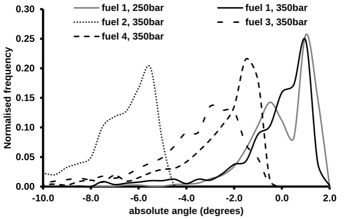
5.3 Flapping spray angles ... 282
Chapter 6 Investigation of diesel jet structure using Laser Induced Fluorescence (LIF) technique ... 291
6.1 Image processing methodology for the phenomenological analysis of the sprays ... 291
v
6.1.2 Spray structure phenomenology ... 292
6.1.3 Liquid Volume Fraction (LVF) distribution along the spray axis ... 294
6.1.4 Asymmetry of the diesel sprays ... 294
6.2 Results and Discussion ... 295
6.2.1 Phenomenological analysis of fully developed diesel sprays... 295
6.2.2 Liquid Volume Fraction (LVF) distribution along the central axis of diesel sprays ... 298
LVF distribution along the spray axis as a function of rail pressure and needle lift 298 5.2.1.2 LVF distributions along the spray axis as a function of fuel’s physical properties 303 6.2.3 LVF distribution across diesel sprays as a function of rail pressure and needle lift ... 308
6.2.4 Spray LVF distributions as a function of the physical properties of the fuels ... 320
Chapter 7 Summary and Conclusions ... 331
Appendix A ... 335
Appendix A1 Sac Vorticity Effects on Nozzle flow – Complementary data and results ... 335
Appendix A2 Correlation between mean in-hole speed and mean in-sac radial flow ... 351
Appendix A3 Buoyant effects as a function of fuel ‘s physical properties. ... 367
Appendix A4 Correlation between in-hole bubble displacement and radial-in sac flow ... 369
Appendix B ... 373
Appendix B1 Filling, emptying, flushing procedures of the fuel injection system ... 373
Appendix B2 Injected mass experimental procedure ... 375
Appendix C ... 376
vi
Table of figures
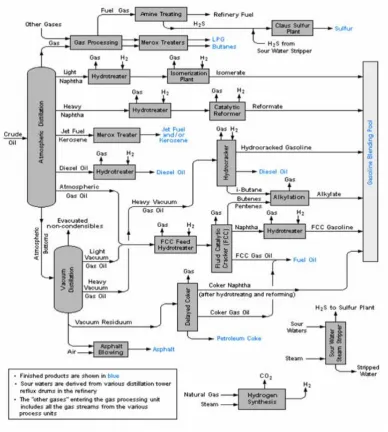
Figure 2.1:Basic schematic of a crude oil refinery system18. ... 30
Figure 2.2:Typical distillation curve of diesel sample ... 32
Figure2.3: Diesel engine characteristics ... 37
Figure 2.4: Schematic diagram of CR injection showing no injection, start of injection and end of injection stages30. ... 38
Figure 2.5: Schematic of the four stages of the cavitation evolution.44 ... 44
Figure 2.6: Caption of the incipient cavitation flow regime53. ... 52
Figure 2.7: Example of pre-film cavitation flow regime53. ... 52
Figure 2.8: Example of film cavitation regime53... 53
Figure 2.9: Example of string cavitation inside an enlarged diesel injector nozzle62. ... 55
Figure 2.10: String cavitation structures linking two neighbouring holes and entering nozzle passages53. ... 56
Figure 2.11: Example of needle string cavitation entering the nozzle passage and extending over the whole length of the nozzle passage56. ... 56
Figure 2.12: Effect of needle lift on spatial and temporal evolution of string cavitation. (a) low needle lift and (b) higher needle lift 68. ... 57
Figure 2.13: Possible causes of FIE deposits79. ... 64
Figure 2.14: Nozzle coking. a) optical observation, b) Microscopic observation81. ... 65
Figure 2.15: Appearance of a typical carboxylate salt85. ... 67
Figure 2.16: Comparison of elements found in IIDs and nozzle-hole deposits83. ... 67
Figure 2.17: Potential formation mechanism of carboxylate salts80. ... 68
Figure 2.18: Typical appearance of organic amide lacquer deposits85... 69
Figure 2.19: TEM images (a and b) of carbonaceous particles90. ... 71
Figure 2.20: Potential deposit formation mechanism8. ... 72
vii
Figure 2.22: Illustration of the near injector region of an atomising spray98. ... 78
Figure 2.23: Basic experimental setup for PDA measurements121. ... 86
Figure 2.24: Optical configurations of Phase Doppler Anemometry. a) annotation of characteristic angles, b) Standard optical configuration124. ... 88
Figure 2.25: Schematic representation of shadowgraphy principles... 90
Figure 2.26: Typical shadowgraph optical arrangement135. ... 91
Figure 2.27: Representation of ballistic, snake and diffuse photos with a) geometric dependence and b) time dependence138. ... 92
Figure 2.28: Shadowgraph images in a dense spray a) with no time gating, b) time gating to supress diffuse light. ... 93
Figure 2.29: Schematic of X-ray absorption experimental setup142. ... 95
Figure 2.30: X-ray images from two different nozzles showing the mass distribution along the spray142,143. ... 96
Figure 2.31: 3-D volume fraction distributions along both radial and axial direction of the spray144. . 96
Figure 2.32: Light scattering by an induced dipole moment due to incident EM wave145 ... 98
Figure 2.33: Diagram showing the intensity of scattered light from different scattering modes152. ... 102
Figure 2.34 : Electronic state diagram illustrating the excitation of an atom to a higher energy level by photon absorption, followed by the emission of fluorescence. ... 104
Figure 2.35: Possible de-excitation pathways of excited molecules158. ... 105
Figure 2.36: Example of singlet and triplet vibrational states158. ... 106
Figure 2.37: Representation of a spatially modulated light traversing a scattering medium172. ... 111
Figure 2.38: An example of 3P-SLIPI application on a cone spray172. ... 112
Figure 2.39: An example of 2P-SLIPI measurement of a premixed Bunsen Flame. a) raw image prior to any correction methods applied, b) processed 2P-SLIPI image174. ... 113
Figure 2.40: Example of averaged 1P-SLIPI technique172. ... 114
Figure 2.41: Index of dependence relation on dye concentration159,148. ... 116
Figure 2.42: Comparison between LSD and PDA measurements148. ... 117
viii
Figure 3.1: Schematic of the custom manufactured fuel injection system16. ... 121
Figure 3.2: Needle lift profiles for a modified Denso injector, Jeshani’s mini-sac nozzle and Makri’s mini-sac nozzle. ... 123
Figure 3.3: Simple designs of: (a) a conventional diesel injector nozzle, (b) modified nozzle with acrylic tip. ... 125
Figure 3.4: Acrylic nozzle cross sections showing the internal dimensions16. ... 125
Figure 3.5: Modified diesel injector nozzle tip showing the view of the holes of interest16. ... 126
Figure 3.6: Injector tip projective transparent view. ... 126
Figure 3.7: Limited optical access through an unpolished surface of the acrylic nozzle. ... 127
Figure 3.8: Polished nozzle surface, providing good optical access to the nozzle passages. The sac is located at the centre of the geometry and the passages entering in the sac are at the same height. .... 128
Figure 3.9: Double acting hydraulic ram16. ... 129
Figure 3.10: Operating principle behind a double acting hydraulic cylinder16. ... 129
Figure 3.11: Injector holder angled at 60 degrees to prevent any interference with the emerging spray16. ... 131
Figure 3.12: Assembly of fuel injection components16. ... 131
Figure 3.13: Image showing the emerging fuel sprays without interfering with the fuel injection assembly16. ... 132
Figure 3.14: Spray extraction design16. ... 133
Figure 3.15: Complete assembly of fuel injection components and fuel exhaust extract16. ... 133
Figure 3.16: Picture showing the cylindrical telescope arrangement and the 50mm mirror. ... 135
Figure 3.17: Picture showing the mirror and lens assembly above the acrylic nozzle tip. The green line shows the laser path. ... 136
Figure 3.18: Schematic of the optical configuration. ... 137
Figure 3.19: Schematic of the internal flow imaging configuration. ... 137
Figure 3.20: Schematic of the LIF/Mie two-channel imaging setup14. ... 139
ix
Figure 3.22: Schematic of synchronisation setup. ... 142
Figure 3.23: Schematic of data acquisition setup... 143
Figure 3.24: Distillation profiles of the fuels under investigation. ... 145
Figure 3.25: Molecular structure of Rhodamine B16 ... 146
Figure 3.26: An example of a laser sheet intensity profile produced by fuel 1 diesel sample. ... 153
Figure 4.1: Frame obtained at 6.0ms after SoI (fuel D) showing the in-sac structures represented by the bright white regions due to white light elastic scattering from the structure interface. (green line: sac volume, red dotted dash profile needle tip, the yellow dashed line: nozzle holes). ... 160
Figure 4.2: (a) Representation of tracking process of an individual structure. y1 to y3 are the y-co-ordinates in three successive frames (nozzle view from the bottom), (b) an example of bubble tracking in a series of raw images (the red circles indicate the bubbles of interest). ... 164
Figure 4.3: Picture of the imaging nozzle side. The yellow dashed lines define the boundaries of the nozzle passages under investigation16. ... 166
Figure 4.4: Images captured between 5.7ms and 6.0ms after the SoI showing the bubble formation in the sac due to needle sheet cavitation (fuel A, 350bar)16. ... 169
Figure 4.5: Vorticity decay rates as a function of fuel physical properties at 250bar over a set of 20 injections. ... 170
Figure 4.6: Vorticity decay rates as a function of fuel physical properties at 350bar over a set of 20 injections. ... 172
Figure 4.7: Examples of a. anti-clockwise and b. clockwise flow direction inside the sac volume16. 173 Figure 4.8: Description of flow direction inside the nozzle passages. ... 176
Figure 4.9: Displacement vs time graph, fuel A at 350bar, lower hole, inj.1-5. ... 178
Figure 4.10: Displacement vs time graph, fuel A at 350bar, lower hole, inj.6-10. ... 179
Figure 4.11: Displacement vs time graph, fuel A at 350bar, lower hole, inj.11-15. ... 179
Figure 4.12: Displacement vs time graph, fuel A at 350bar, lower hole, inj.16-20. ... 180
Figure 4.13: Displacement vs time graph, fuel A at 350bar, upper hole, inj.1-5. ... 180
Figure 4.14: Displacement vs time graph, fuel A at 350bar, upper hole, inj.6-10. ... 181
x
Figure 4.16: Displacement vs time graph, fuel A at 350bar, upper hole, inj.16-20. ... 182
Figure 4.17: Mean speed vs. mean angular speed graph, fuel A, 350bar, inj.1-5, lower hole. ... 183
Figure 4.18: Mean speed vs. mean angular speed graph, fuel A, 350bar, inj.6-10, lower hole. ... 183
Figure 4.19: Mean speed vs. mean angular speed graph, fuel A, 350bar, inj.11-15, lower hole. ... 184
Figure 4.20: Mean speed vs. mean angular speed graph, fuel A, 350bar, inj.16-20, lower hole. ... 184
Figure 4.21: Mean speed vs. mean angular speed graph, fuel A, 350bar, inj.1-5, upper hole. ... 185
Figure 4.22: Mean speed vs. mean angular speed graph, fuel A, 350bar, inj.6-10, upper hole. ... 185
Figure 4.23: Mean speed vs. mean angular speed graph, fuel A, 350bar, inj.11-15, upper hole. ... 186
Figure 4.24: Mean speed vs. mean angular speed graph, fuel A, 350bar, inj.16-20, upper hole. ... 186
Figure 4.25: Experimental bubble speed vs theoretical bubble speed based on buoyancy effects (fuel A, upper and lower passages) ... 188
Figure 4.26: Size distributions of the bubbles and vapour capsules present inside the lower nozzle passage over 50 injections. Each series corresponds to a different fuel. ... 194
Figure 4.27: Size distribution of the bubbles and vapour capsules present inside the upper nozzle passage over 50 injections. Each series corresponds to a different fuel. ... 194
Figure 4.28: A sequence of images produced by fuel sample C showing the progressive break-up of a capsule in the upper nozzle passage during the early stages of post injection16. ... 197
Figure 4.29: A sequence of images produced by fuel sample D showing the progressive break-up of a capsule in the upper nozzle passage during the early stages of post injection16. ... 198
Figure 4.30: A sequence of images produced by fuel sample E showing the progressive break-up of a capsule in the upper nozzle passage during the early stages of post injection16. ... 199
Figure 4.31: Normalised bubble size distribution for fuels A-E at 0.2ms after the needle return. ... 202
Figure 4.32: Normalised bubble size distribution for fuels A-E at 2.2ms after the needle return. ... 202
Figure 4.33: Normalised bubble size distribution for fuels A-E at 4.2ms after the needle return. .... 203
Figure 4.34: Normalised bubble size distribution for fuels A-E at 6.2ms after the needle return. ... 203
Figure 4.35: Normalised bubble size distribution for fuels A-E at 8.2ms after the needle return. ... 204
xi
Figure 4.37: Normalised pressure difference distribution for fuels A-E at 2.2ms after the needle return.
... 205
Figure 4.38: Normalised pressure difference distribution for fuels A-E at 4.2ms after the needle return.
... 205
Figure 4.39: Normalised pressure difference distribution for fuels A-E at 6.2ms after the needle return.
... 206
Figure 4.40: Normalised pressure difference distribution for fuels A-E at 8.2ms after the needle return.
... 206
Figure 4.41: An example of a raw image showing the passage and Region Of Interest (ROI). ... 215
Figure 4.42: SFLVF distributions produced by the mean images obtained from fuel 1 at 250bar (1.8ms,
3.8ms and 5.6ms after SoI) ... 216
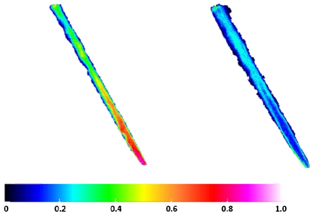
Figure 4.43: Mean false coloured images produced by fuel 1 at 1.8ms, 3.8ms and 5.6ms (left to right)
after SoI and 250bar. ... 217
Figure 4.44: False coloured STD images produced by fuel 1 at 1.8ms, 3.8ms and 5.6ms (left to right)
after SoI and 250bar. ... 217
Figure 4.45: SFLVF distributions produced by the mean images obtained from fuel 1 at 350bar (1.8ms,
3.8ms and 5.6ms after SoI) ... 218
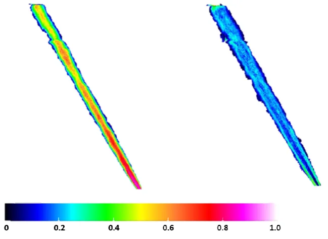
Figure 4.46: Mean false coloured images produced by fuel 1 at 1.8ms, 3.8ms and 5.6ms (left to right)
after SoI and 350bar. ... 219
Figure 4.47: False coloured STD images produced by fuel 1 at 1.8ms, 3.8ms and 5.6ms (left to right)
after SoI and 350bar. ... 220
Figure 4.48: SFLVF distributions produced by the mean images obtained from fuel 3 at 350bar (1.8ms,
3.8ms and 5.6ms after SoI) ... 221
Figure 4.49: Mean false coloured images produced by fuel 3 at 1.8ms, 3.8ms and 5.6ms (left to right)
after SoI and 350bar. ... 221
Figure 4.50: False coloured STD images produced by fuel 3 at 1.8ms, 3.8ms and 5.6ms (left to right)
after SoI and 350bar. ... 222
xii
Figure 5.2: a) An example of a contaminated LIF image, b) an example of a corrected LIF image .. 227
Figure 5.3: Examples of corrected LIF (left hand side) image and Mie image (right-hand side) ... 229
Figure 5.4: Residuals of the ratio of the original mean over the means produced after the sensitivity test
... 230
Figure 5.5: An example of a false colour relative SMD image of the spray (2mm to 18mm) in the range
of 0 - 1.0pixel intensity. ... 231
Figure 5.6: Relative SMD distributions corresponding to sprays produced by fuel A at 250bar and
350bar (1.8ms after SoI). ... 233
Figure 5.7: False coloured mean image produced at 1.8ms after SoI in case of 250bar (left hand side)
and 350bar (right hand side), showing the relative SMD distribution. ... 234
Figure 5.8: False coloured STD image produced at 1.8ms after SoI in case of 250bar (left hand side)
and 350bar (right hand side), showing the variation of the relative SMD distribution from the calculated
mean image. ... 235
Figure 5.9: Relative SMD distributions corresponding to sprays produced by fuel 1 at 250bar and 350
bar (1.8ms after SoI). ... 235
Figure 5.10: Normalised false coloured mean image produced at 1.8ms after SoI in case of fuel 1 at
250bar (left hand) and 350bar (right hand) showing the relative SMD along the spray. ... 236
Figure 5.11: False coloured STD image produced at 1.8ms after SoI in case of fuel 1 at 250bar (left
hand) and 350bar (right hand) showing the variation of the relative SMD along the spray. ... 237
Figure 5.12: Relative SMD distributions corresponding to sprays produced by fuel A at 250bar and
350bar (3.7ms after SoI) ... 238
Figure 5.13: False coloured mean image produced at 3.7ms after SoI in case of 250bar (left hand side)
and 350bar (right hand side) showing the relative SMD distribution. ... 238
Figure 5.14: False coloured STD image produced at 3.7ms after SoI in case of 250bar (left hand side)
and 350bar (right hand side) showing the variation of the relative SMD of the spray droplets. ... 239
Figure 5.15: Relative SMD distributions corresponding to sprays produced by fuel 1 at 250bar and
xiii
Figure 5.16: Normalised false coloured mean image produced at 3.8ms after SoI in case of fuel 1 at
250bar (left hand) and 350bar (right hand) showing the relative SMD along the spray. ... 240
Figure 5.17: False coloured STD image produced at 3.8ms after SoI in case of fuel 1 at 250bar (left
hand) and 350bar (right hand) showing the variation of the relative SMD along the spray. ... 241
Figure 5.18: Relative SMD distributions corresponding to sprays produced by fuel A at 250bar and
350bar (5.6ms after SoI). ... 243
Figure 5.19: False coloured mean image produced at 5.6ms after SoI in case of 250bar (left hand side)
and 350bar (right hand side) showing the relative SMD distribution ... 243
Figure 5.20: False coloured STD image produced at 5.6ms after SoI in case of 250bar (left side) and
350bar (right side) showing the variation of the relative SMD distribution from the calculated mean.
... 244
Figure 5.21: Relative SMD distributions corresponding to sprays produced by fuel 1 at 250bar and
350bar (5.6ms after SoI). ... 245
Figure 5.22: Normalised false coloured mean image produced at 5.6ms after SoI in case of fuel 1 at
250bar (left hand) and 350bar (right hand) showing the relative SMD distribution along the spray. 246
Figure 5.23: False coloured STD image produced at 5.6ms after SoI in case of fuel 1 at 250bar (left
hand) and 350bar (right hand) showing the variation of the relative SMD along the spray. ... 247
Figure 5.24: Relative SMD distributions of the six segments of fuel A spray captured at 1.8ms after SoI,
250bar. ... 248
Figure 5.25: Relative SMD distributions of the six segments of fuel A spray captured at 1.8ms after SoI,
350bar. ... 249
Figure 5.26: Relative SMD distributions of the six fuel 1 spray segments captured at 1.8ms after SoI,
250bar. ... 250
Figure 5.27: Relative SMD distributions of the six fuel 1 spray segments captured at 1.8ms after SoI,
350bar. ... 250
Figure 5.28: Relative SMD distributions of the six fuel A spray segments captured at 3.7ms after SoI,
xiv
Figure 5.29: Relative SMD distributions of the six fuel A spray segments captured at 3.7ms after SoI,
350bar. ... 252
Figure 5.30: Relative SMD distributions of the six fuel 1 spray segments captured at 3.8ms after SoI,
250bar. ... 254
Figure 5.31: Relative SMD distributions of the six segments of fuel 1 spray captured at 3.8ms after SoI,
350bar. ... 254
Figure 5.32: Relative SMD distributions of the six segments of fuel A spray captured at 5.6ms after SoI,
250bar. ... 256
Figure 5.33: Relative SMD distributions of the six segments of fuel A spray captured at 5.6ms after SoI,
350bar. ... 256
Figure 5.34: Relative SMD distributions of the six fuel 1 spray segments captured at 5.6ms after SoI,
250bar. ... 258
Figure 5.35: Relative SMD distributions of the six fuel 1 spray segments captured at 5.6ms after SoI,
350bar. ... 258
Figure 5.36: Relative SMD distribution produced by fuel B at 350bar (3.7ms after SoI). ... 260
Figure 5.37: False coloured mean image (left side) and STD image (right side) produced at 3.7ms after
SoI in case of fuel B at 350bar showing the relative SMD distribution and variation along the spray.
... 261
Figure 5.38: Relative SMD distribution produced by fuel C at 350bar (3.7ms after SoI) ... 262
Figure 5.39: False coloured mean image (left) and STD (right) image produced at 3.7ms after SoI in
case of fuel C at 350bar showing the relative SMD distribution and variation along the spray. ... 263
Figure 5.40: Relative SMD distribution produced by fuel D diesel at 350bar (3.7ms after SoI). ... 264
Figure 5.41: False coloured mean image (left) and STD image (right) produced at 3.7ms after SoI in
case of fuel D at 350bar showing the relative SMD distribution and variation along the spray. ... 265
Figure 5.42: Relative SMD distributions produced by fuel E diesel at 350bar (3.7ms after SoI). ... 266
Figure 5.43: False coloured mean image (left side) and STD image (right side) produced at 3.7ms after
SoI in case of fuel E at 350bar showing the relative SMD distribution and variation along the spray.
xv
Figure 5.44: Relative SMD distribution produced by fuel 2 at 350bar (3.8ms after SoI). ... 268
Figure 5.45: False coloured mean image (left) and STD image (right) produced at 3.8ms after SoI in
case of fuel 2 at 350bar, showing the relative SMD distribution and variation along the spray. ... 269
Figure 5.46: Relative SMD distribution produced by fuel 3 at 350bar (3.8ms after SoI). ... 270
Figure 5.47: False coloured mean image (left) and STD image (right) produced by fuel 3 at 3.8ms after
SoI and at 350bar. ... 270
Figure 5.48: Relative SMD distribution produced by fuel 4 at 350bar (3.8ms after SoI). ... 272
Figure 5.49: False coloured mean image (left) and STD image (right) produced at 3.8ms after SoI in
case of fuel 4 at 350bar, showing the relative SMD distribution and variation along the spray. ... 272
Figure 5.50: Relative SMD distributions of the six spray segments captured at 3.7ms after SoI, fuel B,
350bar. ... 274
Figure 5.51: Relative SMD distributions of the six segments of fuel C spray captured at 3.7ms after SoI,
fuel C, 350bar... 275
Figure 5.52: Relative SMD distributions of the six spray segments captured at 3.7ms after SoI, fuel D,
350bar. ... 276
Figure 5.53: Relative SMD distributions of the six spray segments captured at 3.7ms after SoI, fuel E,
350bar. ... 278
Figure 5.54: Relative SMD distributions of the six fuel 2 spray segments captured at 3.8ms after SoI,
350bar. ... 279
Figure 5.55: Relative SMD distributions of the six fuel 3 spray segments captured at 3.8ms after SoI,
350bar. ... 280
Figure 5.56: Relative SMD distributions of the six fuel 4 spray segments captured at 3.8ms after SoI,
350bar. ... 281
Figure 5.57: Flapping spray angle distributions obtained from fuel 1 at 250bar and 350bar. ... 283
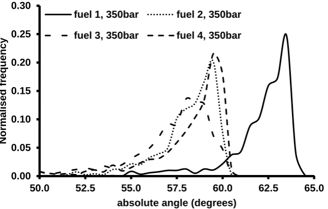
Figure 5.58: Flapping spray angle distributions obtained from fuel 1 to fuel 4 at 350bar. ... 284
Figure 5.59: Flapping spray angle distributions obtained from fuel 1 at 250bar and fuel1 to fuel 4 at
xvi
Figure 6.1: LVF distribution along the fuel A spray central axis produced at 250bar as a function of
needle lift. ... 299
Figure 6.2: LVF distribution along the fuel A spray central axis produced at 350bar as a function of
needle lift. ... 300
Figure 6.3: LVF distribution along the central axis of fuel1 spray at 1.8ms, 3.6ms and 5.6ms after SoI,
250bar. ... 302
Figure 6.4: LVF distribution along the central axis of fuel 1 spray at 1.8ms, 3.6ms and 5.6ms after SoI
after SoI, 350bar. ... 302
Figure 6.5: LVF distributions along the spray axis obtained from fuels B-E at 350bar (3.7ms after SoI).
... 304
Figure 6.6: LVF distributions along the central axis of fue1 sprays 2, 3 and 4 at 3.8ms after SoI, 350bar.
... 306
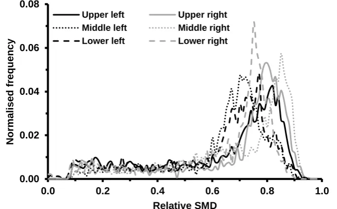
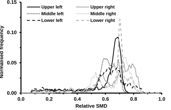
Figure 6.7: LVF distributions of the upper, middle and lower spray segments produced by fuel A at
250bar (1.8ms after SoI). ... 308
Figure 6.8: LVF distributions of the upper, middle and lower spray segments produced by fuel A at
350bar (1.8ms after SoI). ... 309
Figure 6.9: LVF distributions obtained from the upper, middle and lower segments of fuel 1 at 1.8ms
after SoI, 250bar. ... 310
Figure 6.10: LVF distributions obtained from the upper, middle and lower segments of fuel 1 at 1.8ms
after SoI, 350bar. ... 311
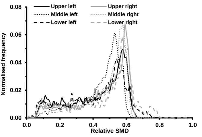
Figure 6.11: LVF distributions of the upper, middle and lower spray segments produced by fuel A at
250bar (3.7ms after SoI). ... 312
Figure 6.12: LVF distributions of the upper, middle and lower spray segments produced by fuel A at
350bar (3.7ms after SoI). ... 313
Figure 6.13:LVF distributions obtained from the upper, middle and lower segments of fuel 1 at 3.8ms
after SoI, 250bar. ... 314
Figure 6.14: LVF distributions obtained from the upper, middle and lower segments of fuel 1 at 3.8ms
xvii
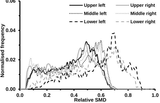
Figure 6.15: LVF distributions of the upper, middle and lower spray segments produced by fuel A at
250bar (5.6ms after SoI). ... 316
Figure 6.16: LVF distributions of the upper, middle and lower spray segments produced by fuel A at
350bar (5.6ms after SoI). ... 317
Figure 6.17: Mean LVF obtained from the upper, middle and lower segments of fuel 1 at 5.6ms after
SoI, 250bar. ... 318
Figure 6.18: Mean LVF obtained from the upper, middle and lower segments of fuel 1 at 5.6ms after
SoI, 350bar. ... 319
Figure 6.19: LVF distributions of the upper, middle and lower spray segments produced by fuel B at
350bar (3.7 ms after SoI). ... 321
Figure 6.20: LVF distributions of the upper, middle and lower spray segments produced by fuel C at
350bar (3.7 ms after SoI). ... 322
Figure 6.21: LVF distributions of the upper, middle and lower spray segments produced by fuel D at
350bar (3.7 ms after SoI). ... 323
Figure 6.22: LVF distributions of the upper, middle and lower spray segments produced by fuel E at
350bar (3.7ms after SoI). ... 325
Figure 6.23: LVF distributions obtained from the upper, middle and lower segments of fuel 2 at 3.8ms
after SoI, 350bar. ... 327
Figure 6.24: LVF distributions obtained from the upper, middle and lower segments of fuel 3 at 3.8ms
after SoI, 350bar. ... 328
Figure 6.25: LVF distributions obtained from the upper, middle and lower segments of fuel 4 at 3.8ms
xviii
List of Tables
Table 2.1: Types of cavitation and their main features42. ... 42
Table 2.2: Summary of internal injector deposits including their root cause, typical appearance and identification80. ... 66
Table 2.3: Mechanism of nozzle fouling91. ... 73
Table 2.4: Illustration of the four main break up regimes along with the associated dominant droplet formation mechanisms94 ... 76
Table 2.5: Criteria of liquid jet disintegration regimes95. ... 77
Table 2.6: Classification of the scattering regimes as a function of optical depth and scattering order. ... 103
Table 3.1: Physical properties of the fuels under investigation. (*R655 additive was believed to introduce viscoelastic properties in the fuels (non-Newtonian fluids)) ... 145
Table 3.2: Summary of camera settings16 (Jeshani’s experiments). ... 149
Table 3.3: Summary of the control unit settings16 (Jeshani’s experiments). ... 150
Table 3.4: Camera inputs and settings. ... 150
Table 3.5: Summary of the nozzle tip used for the fuel testing. ... 152
Table 3.6: Fluorescent yield calibration ratios for RhB fluorescent yield in different fuel mixtures. 154 Table 3.7: Calculated discharge coefficient for all four diesel samples with different nozzle tips. .... 156
Table 4.1: Statistics of the in-sac flow direction for fuels A-E at 250bar and 350 bar. ... 174
Table 4.2: Correlation between the in-hole bubble motion and the radial in-sac motion (fuel A, lower hole). ... 191
Table 4.3: Correlation between the in-hole bubble motion as a function of the radial in-sac motion (fuel A, upper hole). ... 192
Table 4.4: Bubble mean size and pressure difference statistics at 0.2ms, 2.2ms, 4.2ms, 6.2ms and 8.2ms after the needle return (NR). ... 210
xix
Table 5.2: Mean relative SMD values obtained from fuel 1 diesel sprays at 250bar, 350bar (1.8ms after
SoI). ... 251
Table 5.3: Mean relative SMD values obtained from fuel A sprays at 250bar, 350bar (3.7ms after SoI). ... 253
Table 5.4: Mean relative SMD values obtained from fuel 1 diesel sprays at 250bar, 350 bar (3.8ms after SoI). ... 254
Table 5.5: Mean relative SMD values obtained from fuel A sprays at 250bar,350 bar (5.6ms after SoI). ... 257
Table 5.6: Mean relative SMD values obtained from fuel 1 sprays at 250bar, 350bar (5.6ms after SoI). ... 259
Table 5.7: Mean relative SMD values obtained from fuel B sprays at 350 bar (3.7ms after SoI). ... 274
Table 5.8: Mean relative SMD values obtained from fuel C sprays at 350 bar (3.7ms after SoI). ... 276
Table 5.9: Mean relative SMD values obtained from fuel D sprays at 350 bar (3.7ms after SoI). ... 277
Table 5.10: Mean relative SMD values obtained from fuel E sprays at 350bar (3.7ms after SoI). .... 278
Table 5.11: Mean relative SMD values obtained from fuel 2 diesel sprays at 350 bar (3.8ms after SoI). ... 279
Table 5.12: Mean relative SMD values obtained from fuel 3 diesel sprays at 350 bar (3.8ms after SoI). ... 281
Table 5.13: Mean relative SMD values obtained from fuel 4 diesel sprays at 350 bar (3.8ms after SoI). ... 282
Table 5.14: The actual nozzle passage angle measured from the magnified nozzle images and the mean absolute angle calculated based on the spray data. ... 286
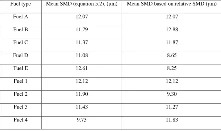
Table 5.15: Mean SMD of the droplets produced by fuels A-E anf fuels 1-4 at 350bar, based on the empirical relationship and the relative SMD values. ... 288
Table 6.1: Location of primary atomisation onset (mm) for fuels A to E and 1to 4. ... 296
xx
Table 6.3: Mean LVF obtained from the upper, middle and lower segments of fuel 1 at 1.8ms after SoI,
250bar. ... 312
Table 6.4: Mean relative LVF values obtained from fuel A sprays at 250bar, 350bar (3.7ms after SoI). ... 313
Table 6.5: Mean LVF obtained from the upper, middle and lower segments of fuel 1 at 3.8ms after SoI, 350bar. ... 316
Table 6.6: Mean relative LVF values obtained from fuel A sprays at 250bar, 350 bar (5.6ms after SoI). ... 317
Table 6.7: Mean LVF obtained from the upper, middle and lower segments of fuel 1 at 5.6ms after SoI, 350bar. ... 320
Table 6.8: Mean relative LVF values obtained from fuel B spray at 350 bar (3.7ms after SoI). ... 321
Table 6.9: Mean relative LVF values obtained from fuel C sprays at 350 bar (3.7ms after SoI). ... 323
Table 6.10: Mean relative LVF values obtained from fuel D spray at 350bar (3.7ms after SoI). ... 324
Table 6.11: Mean relative LVF values obtained from fuel E spray at 350bar (3.7ms after SoI). ... 325
Table 6.12: Mean LVF obtained from the upper, middle and lower segments of fuel 2 at 3.8ms after SoI, 350bar. ... 327
Table 6.13: Mean LVF obtained from the upper, middle and lower segments of fuel 3 at 3.8ms after SoI, 350bar. ... 329
xxi
Acknowledgements
First of all, I would like to thank my supervisor Dr Russel Lockett who gave me the opportunity to work
on such a challenging and interesting project. This dissertation would not have been possible without
his guidance, support and advice. I would also wish to thank Shell Global Solutions for funding this
project.
I would like to acknowledge the technicians of City, University of London: Mr Rob Cherry, Mr Grant
Clow and Mr Jim Ford, who delivered complicated requests and were always willing to help me in
resolving problems during the execution of my experiments. I would also like to thank Professor John
Carlton and Professor Jamshid Nouri for giving me permission to use their equipment and providing
me with useful tips. Lastly, I would like to acknowledge Dr Olawole Kuti ‘s contribution who inspired
me to compose my first publication and shared useful tips and material with me.
I owe a debt of gratitude to my colleagues Alberto and Zeeshan, who have become my closest friends
during this journey at City. Their moral support and useful conversations cheered me up when I needed
it the most. I would also like to mention all my friends and colleagues with whom I shared the PhD
office and lunch times: Yannis, Elina, Kostas, Antonio, Eleni, Saeed, Dimitris and Israt. Lastly, I
genuinely thank all my friends Nancy, Palmyra, Agni, George, Stavros, Athina and Elena who bore
with me patiently during all this time and supported me in any possible way.
Finally, I could not forget to thank all my family back home who kept supporting and encouraging me
xxii
Abstract
The advances in Fuel Injection Equipment have increased the injection and combustion efficiency, but have also increased the possibility of failure. Recent studies have identified various types of deposits of different components, such as fuel filters, injector nozzles etc. In this regard, white light scattered from the internal flow structures along with both elastic (Mie signal) and inelastic light (fluorescence) from the external sprays were synchronously captured by two separate high-speed cameras. The part of the present work was based on the experiments conducted by Jeshani Mahesh and post-processed by the author of this dissertation. The analysis performed suggested potential deposit formation mechanisms inside diesel injector nozzles considering the operating conditions of the injection system and the physical properties of the fuels. The observed circumferential bubble motion at the late stages of the needle return and post-injection, has been proven to generate low and high-pressure gradients which govern the bubble movement inside the nozzle passages. In engine conditions, the inward bubble movement inside the passages is believed to be the mechanism for the admission of hot combustion gases inside the nozzle geometry. The reaction of these hot gases with the liquid fuels is believed to produce deposits inside the FIE. The LIF-Mie obtained ratios provided an insight into the external spray drop-sizing and atomisation characteristics. The undertaken analysis revealed a strong link between the spray drop size and the physical properties of the fuels. It was also shown that both the needle lift and the operating conditions played a decisive role in the atomisation process and that an increase in rail pressure led to the formation of smaller droplets, while an increase in viscosity and surface tension led to larger droplets. The size of the spray droplets during the early and late stages of the needle lift was larger in relation to the maximum needle lift, due to the synergy of flow chocking and various types of cavitation (needle cavitation, string cavitation). The final section of this analysis involves the phenomenological study of the emerging sprays based on the LIF spray data. This study that the liquid core of the sprays was destroyed either inside the nozzle passage or in the vicinity of the nozzle exit. The obtained results referred to the LVF of different regions of the sprays as a function fuels’ properties, needle lift and rail pressure.
xxiii
Abbreviations
ac: Amplitude of modulated light
ASTM: American Society for Testing Materials
CCD: Charge Coupled Device
Cd: Discharge coefficient
CN: Cetane Number
CO: Carbon monoxide
CO2: Carbon Dioxide
CFR: Cooperative Fuel Research
CR: Common Rail
dc: Amplitude of non-modulated light
DCA: Deposit Control Additives
DDSA: Dodecenyl Succinic Acid
DI: Direct Injection
ECC: Enhanced Correlation Coefficient
EDS: Energy Dispersive X-Ray Spectroscopy
EM: Electro-Magnetic
FAME: Fatty Acid Methyl Esters
FIE: Fuel Injection Equipment.
FTIR: Fourier Transform Infrared Spectroscopy
FWHM: Full Width Half Maximum
GTL: Gas To Liquid
HC: HydroCarbons
HDSA: Hexadecenyl Succinic Acid
HOMO: Highest Occupied Molecule Orbitals
HPLC: High Performance Liquid Chromatography
IDI: Indirect Injection
IID: Internal Injector Deposits
INF: INternal Flow
lc: Length of the spray liquid core
LC: Liquid Chromatography
LDA: Laser Doppler Anemometry
LDV: Laser Doppler Velocimetry
LIF: Laser Induced Fluorescence
LSD: Laser Sheet Drop-sizing
LUMO: Lowest Unoccupied Molecule nOrbitals
LVF: Liquid Volume Fraction
MS: Mass Spectroscopy
NaOH: Sodium hydroxide
NI: National Instruments
NOx: Nitrogen Oxide
NR: Needle Return
OD: Optical Density
Oh: Ohresorge
PAH: Polycyclic Aromatic Hydrocarbons
PIBSA: Polyisobutylene anhydrite
PIBSI: Polyisobutylene succinimide
RhB: Rhodamine B
SEM: Scanning Electron Microscopy
SFLVF: Scattered Fluorescence Liquid Volume Fraction
SIC: Single Ion Chromatographs
SLIPI: Structured Laser Illumination Planar Imaging
SMD: Sauter Mean Diameter
SNR: Signal to Noise Ratio
SoI: Start of Injection
STD: Standard deviation
VCO: Valve Covered Orifice
24
Chapter 1
Introduction
The increasing demand of energy and mobility in contrast to the limited resources of fossil fuels and
the environmental concerns with regards to global warming and air pollution have led to the
development of new, cleaner and more efficient technologies for energy production. In the past decades,
the research community has focused its attention on the development of new propulsion systems
including advanced processes and highly efficient, environmental friendly fuels. In this regard,
significant efforts have been made on the sufficient understanding the fundamental physics of major
processes (i.e. combustion, atomisation) taking place in diesel engines. One of the biggest advances of
the modern diesel engines is the introduction of efficient high-pressure common rail injection systems,
which provide great flexibility in terms of engine control and management over a wide spectrum of
operating conditions and fuels.
The employment aim of such systems is the enhancement of the atomisation process and the delivery
of accurate, precise and optimal air-fuel mixtures to the combustion chamber. It has been suggested1
that there is a strong correlation amongst the atomised diesel fuels, the combustion and thermal
efficiency and the engine-out emissions. Therefore, a thorough study of the atomisation process is
essential to obtain a suitable optimal range of the parameters capable of improving the fuel-air mixing
process and subsequently resulting in reduced emissions. However, the scientific and industrial interest
in spray characterisation barely existed a few decades ago, due to its complexity and lack of suitable
facilities and experimental techniques. Nowadays, the development of technology (i.e. high-speed
cameras, lasers etc) together with the many applications of sprays to various industries (i.e. aviation,
agricultural, automotive) have promoted the development of suitable optical diagnostics for spray
characterisation.
The most significant example of spray application concerns the injection of liquid fuel into pistons
25
to large pressure gradients, which in turn cause local boiling conditions. This is likely to occur when
the pressure drops below the saturated vapour pressure of the fuel. Under such conditions, the fuel state
changes into vapour creating local vapour cavities. This phenomenon is known as cavitation. A
cavitating flow has been suggested to affect the structure of the emerging sprays, the atomisation
process and the lifetime of the FIE2,3. It has also been shown experimentally that cavitation modifies
significantly the injector surfaces, possibly due to hydro-erosion and hydro-grinding4. Additionally,
cavitation is believed to be dependent on the physical properties of the fuels. Several researchers4,5 have
reported that fuel samples containing Fatty Acid Methyl Esters (FAME) have the tendency to cavitate
less in relation to the conventional diesel.
The demand for better combustion and atomisation efficiency has led the FIE industry to develop
systems that operate at extreme pressure conditions. World leading injector manufacturers such as
Bosch, Denso have reported the development of common rail injection systems capable of achieving
pressures of up to 3,000bar6,7. The extreme temperature and pressure conditions generated together with
the small dimensions of the nozzle passages create conditions that are able to support the formation of
injector deposits via pyrolysis reactions, chemical re-arrangement or the fuel decomposition. These may
lead to nozzle blockage or even failure. The synergy of the extreme operating conditions together with
the introduction of new fuel blends (low sulphur content fuels blended with a wide range of additives
and biofuels) has led to an increase in the incidents of injector fouling. Indeed, several authors 8–12have
reported the existence of deposits at various points of the injector geometry such as hole entrance,
needle, nozzle sac etc., while others have made attempts to suggest potential mechanisms for deposit
formation8,13. However, the results and the models developed so far are not conclusive. It has been
suggested that atomisation and internal flow are greatly affected by the presence of deposits, which can
potentially lead to increased fuel consumption, power loss and equipment failure15. The effect of
cavitation in deposit formation appeared to be beneficial for the removal of deposits from diesel
injectors.
Apart from the impact of the fuel’s physical properties on cavitation, it has been experimentally
26
droplet size, spray cone angle etc.14,15. In practice, atomisation is the result of the dominant effects of
the internal or external forces over the stabilizing effects of the viscosity and surface tension of the fuel.
Some of the most significant parameters contributing to the atomisation process are cavitation, flow
turbulence and fuel properties. Depending on the stage of the liquid disintegration and droplet stability,
atomisation can be classified into primary and secondary atomisation. In most cases, the liquid
break-up is an unstable and complex physical process, which is difficult to control and investigate. The first
approach in investigating such complex systems was the primary identification of the spray properties
(i.e. droplet size, spray cone angle, spray penetration length etc) under a range of different operating
conditions.
In the last few decades, the spray characterisation was initially achieved using mechanical or electrical
devices, but more recently optical techniques have become the methods of choice, due to their remote
sensing, non-intrusive nature and the availability of a wide variety of instruments suitable for spray
measurements. However, each of these optical diagnostics serve a different purpose and provide
specific and/or local information. Some of them provide general information with regards to the
structure and geometry of the spray, while some others to the size, velocity, temperature of the spray
droplets. Additionally, some other techniques are employed to investigate the spray break-up
mechanisms (primary and secondary break-up mechanisms) and atomisation. In many cases, the
combination of more than one method is usually required for a complete spray characterisation. On the
other hand, despite the profound advantages of these techniques, there are cases, such as dense spray
regions, where their application and performance are doubtful.
The present work involved experimental data obtained from two individual experiments. The first set
of experiments was executed by Jeshani16 and the second set by the author of this dissertation. The data
processing was based on Jeshani’s work, but it has been further developed and improved by this thesis’s
author.
The objective of this work was to comprehensively investigate the external structure of the atomising
sprays emerging from a custom manufactured, real-sized, 6-hole, optically accessible mini-sac type
27
using optical diagnostics. The analysis performed on Jeshani’s data was focused on the investigation of
the external spray droplet size and phenomenology using Laser Sheet Drop-sizing and Laser Induced
Fluorescence techniques respectively. It was also attempted to suggest potential deposit formation
mechanism based on the post-injection phenomena occurring in the sac and the nozzle holes. The
experimental method used for the identification of internal flow features was white light scattering
(elastic scattering).
The analysis based on the experimental work of this thesis’s author attempted to primarily improve the
previous experiment by replacing white light scattering with Laser Induced Fluorescence (LIF)
technique. This method is capable of providing quantitative measurements of the liquid volume faction
inside the nozzle passage during the injection process and to identify flow features, such as geometric
cavitation. Similarly to Jeshani’s data, the spray characterisation was achieved using Laser Sheet
Drop-sizing technique, providing the opportunity to evaluate the results obtained by comparison. To the best
of the author’s knowledge, the application of LIF in real-sized, mini-sac nozzles was attempted for the
first time, therefore this work could be considered original and novel.
A key aspect of this investigation was the identification of the correlation amongst the internal flow,
the external sprays and the physical properties of the fuels, as a function of the transient movement of
the injector needle and the operating conditions (the experiments were performed at 250bar and 350bar).
Jeshani’s results were obtained from five diesel fuel samples, while the second set of results from four
diesel samples. The majority of the fuels used had similarities in terms of their physical properties (i.e.
distillation profile, viscosity etc). All fuel samples were provided by Shell Global Solutions.
The work presented in this dissertation was distributed into 7 Chapters. A brief summary of the content
of each Chapter individually is listed below.
Chapter 2 provides a detailed literature review of the fields related to this work. Initially, it provides a
quick overview over the fundamentals of diesel fuels and injection systems. It describes the
fundamentals of cavitation and atomisation processes and the optical diagnostics suitable for their
28
experimental setup, apparatus, high speed acquisition setup and timing, laser sheet drop-sizing
setup, experimental and calibration methodologies were described in Chapter 3. Chapter 4 involved
the detailed description of the internal flow data obtained from both white light and fluorescence
scattering experiments respectively. The results from both experiments were presented and
discussed in detail.
Chapter 5 and 6 referred to the characterisation of the diesel sprays in terms of the droplet size and
liquid volume fraction using the Laser Sheet Drop-sizing and Laser Induced Fluorescence
experimental data. It involved the detailed description of the processing methodologies used and
the discussion of the results obtained from both experiments, which highlighted the dependence of
the droplets size on the physical properties of the fuels, the transient movement of the needle and
the injection pressure.
Lastly, Chapter 7 provided an overview of the conclusions drawn from the analyses together with
29
Chapter 2
Literature review
This section was devoted to the reviews of the fundamentals of diesel fuels, diesel injection systems,
cavitation, atomisation and deposit formation processes together with a detailed description of the
optical techniques widely used for internal flow and spray characterisation. The aim was to familiarise
the reader with the most dominant processes and terms elaborated in this work.
2.1
Diesel fuel backgroundDiesel fuel is one of the most common fossil fuels utilised for industrial, domestic and agricultural
purposes. The combustion produces sufficient chemical energy which in turn is converted into
mechanical energy. In this section the production, composition and performance parameters of diesel
fuels and diesel engines were discussed. The literature review was mostly based on Srivastava, Hancsó17
and other technical reports found online. The description of the fuel refinement processes was also
presented in order to highlight the main production processes and therefore, provide an insight of the
fuel composition and properties. The understanding of the physical properties of the fuels was essential
for this work, as they related to the work presented in later chapters. Additionally, the effects of the
performance parameters on the fuel properties and their impact on various processes (i.e. cavitation,
atomisation, combustion) taking place in Fuel Injection Equipment (FIE) were also reported.
Ultimately, the discussion of currently used alternative fuels and fuel additives was presented at the end
of this chapter to provide information about fuel’s performance.
Refinery process of crude oil and diesel fuel composition.
Diesel fuel comes from the refinement of crude oil. Crude oil is mainly composed of carbon (83-87%
w/w), hydrogen (11-14% w/w) and small traces of other elements (e.g. sulphur). It varies from thin,
light coloured, brownish or greenish crude oils (low density, high gravity) to thick, black oils (high
density, low gravity). The petroleum crude oil is refined to produce various fuels such as diesel,
30
conversion processes. The first two stages refer to processes that do not change the chemical structure
of the crude oil, while the last one significantly changes its molecular structure. A simple schematic of
[image:31.595.103.492.157.590.2]a crude oil refinery plant is shown in Figure 2.1
Figure 2.1:Basic schematic of a crude oil refinery system18.
Initially, crude oil undergoes a separation process which is based on the nature of the hydrocarbons in
terms of their physical properties (i.e. volatility). The most common separation process is distillation,
and in the refinery industry it can be processed at either atmospheric pressure or vacuum. In the case of
atmospheric distillation process, crude oil is separated into a wide range of products with narrow boiling
31
heated into a heat exchange train, it then enters the distillation column as a gas-liquid mixture. The more
volatile, light components rise upwards, while the heavier compounds are being condensed by the cold
down flow of liquid fuel. These light components exit the column at the top, where they are subjected
to condensation such that light gases (C1-C4) and light naptha are obtained. The purity of these light
products is later improved in other units of the refinery plant, employing several methods (i.e. stripping).
The rest of the hydrocarbon mixture has higher boiling point and does not reach the top of the column.
In particular, gasoline is drawn off from the side of the column while kerosene and diesel (higher boiling
points relative to gasoline) are drawn off successively lower from the distillation column. The oil
residue is in liquid phase and consists of the heaviest components; therefore; it exits the column at the
bottom.
This primary separation process is then followed by several upgrading processes which aim to improve
the quality of the distillates by removing undesirable compounds present into the fuels. The most
common upgrading process is hydro-treating, which is employed to a) remove oxygen and sulphur
compounds via chemical reactions involving hydrogen and b) to saturate aromatic rings and to eliminate
the amount of nitrogen and sulphur compounds left in the distillates. After the upgrade processes, the
fuel is subjected to conversion processes which are utilised to perform changes in the chemical structure
of the hydrocarbons and eventually to meet the desired requirements in terms of fuel quality. This
conversion involves methods which either alter the number of the carbon molecules in the hydrocarbons
or produce molecules of more useful hydrocarbon molecules. Some of the most common processes
related to conversion of hydrocarbon without any changes in the carbon molecule population are
de-sulfurization and skeletal isomerization. On the other hand, the methods utilised for the conversion of
hydrocarbon structures into compounds of higher or lower number of carbon molecules are
oligomerization or several types of cracking respectively (i.e. catalytic cracking, thermal cracking etc.).
In this work, the focus is on middle distillate products whose distillate profiles are similar to diesel fuel.
In general, diesel fuels are mixtures of crude oil derived and alternative blending components. Such
32
have to comply with very specific requirements; therefore, it is essential to employ certain refinery
technologies along with a carefully selected range of additives and complex processing methods.
Composition and properties of diesel fuel
Diesel fuel is a mixture of thousands of hydrocarbons obtained through the fractional distillation of
petroleum fuel oil, with a boiling point in the range of 175-350oC. Due to its complexity, diesel oil
cannot be characterised by a single well-defined boiling point, but by a boiling point range and by
temperature values related to the distilled fraction. A typical distillation curve of a diesel sample is
shown in Figure 2.2.
Figure 2.2:Typical distillation curve of diesel sample
Crude oil derived diesel fuels have a composition of approximately 75% aliphatic hydrocarbons and
25% aromatic hydrocarbons. The most common hydrocarbon classes found in such fuels are paraffins,
olefins, napthenes and aromatic rings. Each class of hydrocarbons has different physical and chemical
properties; hence each blend of diesel fuel is different from other blends due to each having different
proportions of these classes. The most important fuel properties are the distillation curve, density,
surface tension, cetane number and viscosity, which vary depending on their relative proportions of
classes of hydrocarbons19.
150 175 200 225 250 275 300 325 350
0 10 20 30 40 50 60 70 80 90 100
T
emp
er
atu
re
(o
C)
Volume (%)
33
A fundamental parameter of fuels is the distillation curve (boiling point curve) which is experimentally
determined using ASTM-D86 method. By increasing the temperature, more volatile components may
be reduced, while the heavier may be caught by the lighter ones. The range of boiling point for diesel
fuels is quite wide and significantly affects properties such as viscosity, density, ignition delay and
flashpoint. It also determines the applicability and the behaviour of fuels in the engine. Deposit
built-up in engines is influenced by excessive amounts of high-boiling point compounds. Thus, limitations
are set on carbon residue and the distillation product at 90% evaporated temperature20.
Cetane Number (CN) defines the quality of the fuel in terms of its ignition. In other words, it is a
measure to quantify the propensity of the fuels to burn under diesel engine conditions. The cetane
number also offers an estimate with regards to the ignition delay period, namely the time period between
the start of the injection and the first moment where the combustion pressure developed in the
combustion chamber becomes noticeable. A rapid increase of the pressure, as a result of the rapid heat
release due to combustion, is responsible for the characteristic combustion occurring after the initial
delay. Therefore, fuels with high cetane number ignite shortly after the fuel injection into the cylinder
resulting in a smooth, quiet engine run, but it is not necessarily more efficient. On the other hand, fuels
with relatively low CN resist auto-ignition and present a longer ignition delay period. The latter is a
very important parameter that required careful adjustment. In the case of a very long ignition delay, the
combustion of the fuels occurs violently while in case of a short ignition delay, the fuel ignites before
achieving adequate mixing and consequently the amount of the emitted gases increases. Lastly, CN is
a valid ignition delay measure only in cases of a single cylinder engines. The most widely methods used
for the determination of Cetane number is the traditional ASTM D613 and the ASTM D6890 methods21.
The traditional ASTM D613 method evaluates the ignition quality of diesel samples. The fuel samples
are inserted into a variable volume combustion chamber of a Cooperative Fuel Research (CFR) engine
where the compression ratio is regulated to produce a standard ignition delay of 13o after the top dead
centre (farthest piston position from the crankshaft). Lastly, the determination of the fuel quality is
achieved by comparing the corresponding ignition delay to the reference fuel
On the other hand, the ASTM D6890 method provides a more modern approach in evaluating the
34
employs a fixed combustion chamber to measure the ignition delay. Then the measured values are
substituted into correlation equations to obtain the derived cetane number. The experimental apparatus
used for the execution of this method is called Diesel Fuel Ignition Quality Tester. Both methods
provide comparable results; the latter is capable of evaluating fuels that the traditional method cannot
measure.
Therefore, in case of tests in real engines, two other methods are utilised to serve this purpose: The
Cetane Index(CI)Reference 22 and the Diesel Index (DI) methods.
The Cetane Index (CI) provides an estimate of the ASTM cetane number (D613) of distillate fuels
utilising density and distillation recovery temperature measurements23. It is a supplementary tool for
estimating the cetane number when a test engine is not applicable and if a cetane improver is not used.
CI is not valid in cases of pure hydrocarbon mixtures, residual fuels, synthetic fuels or coal tar products.
The calculation of the CI can be achieved using Equation 1.1.
10 50 90 50
2 2 2
90 10 90
CI
45.2 0.0892 T
215
0.131 T
260
0.05823 T
310
0.901B T
260
0.420B T
310
0.0049 T
215
0.0049 T
310
107B 60B
Equation
2.1
Where [ 3.5 D 0.85 ]
Be , D: the specific gravity at 15oC and Tx: x% distillation temperatures.
The Diesel Index (DI) is a measure of the ignition quality of a diesel fuel calculated from a formula
involving the gravity of the fuel and its aniline point. Its mathematical approach is shown in Equation
2.2.
Equation 2.2
The aniline point is the minimum temperature of complete miscibility of an equal volume of aniline and
a test sample. The higher the aniline point is the higher paraffinic content or lower the aromatic content
of the fuel.
Volatility is the tendency of a substance to vaporize and is directly related to fuel’s saturated vapour
pressure. It is expressed in terms of the temperature (T95) at which 95% of the sample is evaporated and
presents a measure of the least volatile component present in the fuel sample24. At a given temperature,
a fuel with a higher saturated vapour pressure vaporizes easier than a fuel with a lower saturated vapour
aniline po int*gravity
DI
100
35
pressure. Therefore, in case of a highly volatile fuel, the transition from the liquid to the vapour state
could take place at any time inside the fuel delivery system and subsequently result in vapour lock
phenomenon and possibly in lower flash point. The flash point of a volatile material is the lowest
temperature at which it can vaporize to form an ignitable mixture in air. Hence, fuels with a low flash
point have shown an adverse effect on safety in handling and storage, while high flash point fuels seem
to have an increased propensity to form deposits and smoke and cause wear in various parts of the
equipment. It is evident that volatility is an important parameter which greatly affects the engine
emissions. In particular, when reducing the T95, the amount of the NOx emissions is decreased, while
the amounts of the emitted hydrocarbons and CO are increased. However, the proportion of the emitted
PMs seems to be independent from such a reduction20.
The density of a substance is defined as the fraction of its mass per volume unit. The density of diesel
fuels directly influences the volumetric energy content (lower heating value), which in turn influences
the driving moment as a function of the revolution. With higher density and same injection volume,
engines provide higher performance as a result of the higher energy content; hence, with increasing
density the acceleration of the vehicle will be higher. On the other hand, a reduction in fuel density
leads to less NOx emissions in Indirect Injection (IDI) diesel engines; however, emissions obtained from
modern Direct Injection (DI) diesel engines do not seem to be sensitive to density changes20,22.
In principle, the viscosity of a fluid is defined as a measure to quantify its resistance to the gradual
deformation by shear stress or tensile stress. In fuels particular, it is primarily related to molecular
weight and not so much to the hydrocarbon class. It also plays an important role in achieving good
performance of the fuel injection system, in terms of fine atomisation and good lubrication of the fuel
supply system. High viscosity fuels cause wear in the fuel injection pump, reduced atomization and
vaporization of fuel, while fuels with lower viscosity decrease the velocity gradients developed inside
the nozzle geometry17 and also they may lead to less intensive cavitation phenomena and consequently
to poorer atomisation. Finally, the viscosity determines the size of the droplets and the penetration of
the diesel spray5.
Surface tension has been reported25 to be one of the most important parameters in the atomization