A time-domain Green's function for interaction betweenwaterwaves and floating bodies with viscous dissipation effects

City, University of London Institutional Repository

Citation

:

Guo, Z., Ma, Q. & Qin, H. (2018). A time-domain Green's function for interaction

betweenwaterwaves and floating bodies with viscous dissipation effects. Water, 10(1), doi:

10.3390/w10010072

This is the published version of the paper.

This version of the publication may differ from the final published

version.

Permanent repository link:

http://openaccess.city.ac.uk/18968/

Link to published version

:

http://dx.doi.org/10.3390/w10010072

Copyright and reuse:

City Research Online aims to make research

outputs of City, University of London available to a wider audience.

Copyright and Moral Rights remain with the author(s) and/or copyright

holders. URLs from City Research Online may be freely distributed and

linked to.

City Research Online:

http://openaccess.city.ac.uk/

[email protected]

Article

A Time-Domain Green’s Function for Interaction

between Water Waves and Floating Bodies with

Viscous Dissipation Effects

Zhiqun Guo1_{, Q. W. Ma}1,2_{and Hongde Qin}1,_*

1 _{College of Shipbuilding Engineering, Harbin Engineering University, Harbin 150001, China;}

[email protected] (Z.G.); [email protected] (Q.W.M.)

2 _{School of Engineering and Mathematical, City University London, London EC1V 0HB, UK} * Correspondence: [email protected]; Tel.: +86-137-0451-3212

Received: 23 December 2017; Accepted: 12 January 2018; Published: 15 January 2018

Abstract: A novel time-domain Green’s function is developed for dealing with two-dimensional interaction between water waves and floating bodies with considering viscous dissipation effects based on the “fairly perfect fluid” model. In the Green’s function, the temporal (lower order viscosity coefficient term) and spatial (higher order viscosity coefficient term) viscous dissipation effects are fully considered. As compared to the methods based on the existing time-domain Green’s functions that could not account for the spatial viscous dissipation, the method based on the new time-domain Green’s function can give much better numerical results and overcome instability problems related to the existing Green’s function, according to the numerical tests and comparison with CFD modeling data for a few cases related to floating bodies with a flare angle.

Keywords: water waves; Green’s function; viscous dissipation effects; interaction between water waves and floating bodies

1. Introduction

The interaction between water waves and floating bodies is one of most common occurrences in marine or ocean engineering. The interaction could induce ships or floating platforms to make six degree of freedom (6-DOF) motions, and wave loads may bring damage for the structures. Therefore, it is of great significance to investigate the interaction between water waves and floating bodies. There are many numerical methods that could be employed for such purpose, such as Green’s function methods, finite element methods, meshless methods and so on. Among these methods, Green’s function methods are most efficient because they are linear panel methods with panels or segments distributed only on the wetted surface of floating bodies.

As a result of ignoring fluid viscosity, the conventional inviscid Green’s function methods encounter difficulties in solving some water surface hydrodynamic problems associated with viscosity, such as the decay of gravity waves during propagating and exact amplitude of resonant waves in shielded waters. To overcome those, two main viscous correction models are proposed in the literature to improve the Green’s function methods. In these two models, Green’s functions are obtained by solving boundary value problems with viscous correction (BVP_V), in which the free-surface conditions are corrected by a viscous dissipation term, while other conditions remain the same as the inviscid ones.

The first model is based on the “fairly perfect fluid” [1], where the dissipation term in the linear momentum equation is−υ∇ψ(υ ≥0 is an artificial viscosity coefficient). In this model, the linear

Bernoulli’s equation and free-surface condition with viscous dissipation term can be, respectively, written as [1,2]

 



∂ψ ∂t +

p

ρ+gη+υψ=0 ∂2ψ

∂t2 +g ∂ψ ∂y +υ

∂ψ ∂t =0

(1)

The second model is based on the linear incompressible NS equations, from which the linear Bernoulli’s equation and free-surface condition can be, respectively, deduced as follows [3,4]

 



∂ψ ∂t +

p

ρ+gη+2ν ∂2ψ ∂y2 =0 ∂2ψ

∂t2 +g

∂ψ ∂y+4ν

∂3ψ ∂t∂y2 =0

(2)

whereoyaxis points upward; andνandψare physical kinematic viscosity coefficient and velocity potential of the fluid, respectively.

For the sake of distinction, in this paper, the Green’s function derived using the first and second models are called the first and second kind of Green’s function with viscous dissipation effects ( GF1_V and GF2_V), respectively. Although the viscous dissipation term in Equation (1) is simpler than that in Equation (2), it was indicated [4] that the two viscous correction approaches are equivalent to each other due to the relationship between the artificial viscosity coefficientυand the physical kinematic viscosity coefficientν:υ=4νk2, wherekis the wave number.

Although the viscous dissipation term in Equations (1) or (2) is linear with respect to the viscosity coefficient, the exact Green’s function with viscous dissipation effects (GF_V) derived from the BVP_V is nonlinear to it. Nonetheless, nearly all GF_V proposed in the literature only exactly contain the lower order viscosity coefficient term, while the higher order ones are not fully considered. Admittedly, the GF_V with lower order viscosity coefficient term (GF_V1) are sufficient to solve general water wave problems, since in these problems the viscosity coefficients are low enough (the same as or analog to real viscosity of water) to make the high order viscosity coefficient terms insignificant. The major works in this respect are enumerated as follows. Chen [2] first proposed a GF1_V1to eliminate the numerical resonance phenomena in multi-body hydrodynamics, and a similar work was followed [5]. Then, a GF2_V1was developed to analyze the time-harmonic ship waves [4]. Further, a tank GF2_V1 was presented for investigating the realistic effects of water viscosity and side walls on waves in tanks [6].

The GF_V1, however, should not be appropriate for solving the hydrodynamic problems associated with larger fluid viscosity (e.g., the sloshing of oil in the cargo tank) or with vortex shedding around sharp edges of floating bodies, the later of which accompanies with significant fluid pressure and flow energy loss. This is because the viscous dissipation effects in such cases are so large that the higher order viscosity coefficient terms in GF_V cannot be ignored. Nevertheless, several attempts of applying GF_V1on solving such problems were also made in some works. Chen et al. [7] set a dissipation surface from the sharp edge of a moonpool down to the seabed, imposed a continuous flow velocity but a discontinuous pressure across this dissipation surface to simulate the pressure loss near the sharp edge, and then employed a GF1_V1to solve the BVP_V. Analogously, Cummins and Dias [8] proposed a pressure discharge model to evaluate the viscous dissipation effects near a flap’s edge. One should notice that in these two works the GF_V1was not used alone but in combination with additional pressure correction models in the vicinity of sharp edges.

with the physical viscosity of water to study a cone heaving on the water surface. Wu’s failure mainly results from the weak viscosity of water and without consideration of higher order viscosity coefficient terms in TGF2_V1. Similar to the vortex shedding cases, one should artificially enlarge the viscosity coefficient in TGF_V, as well as take the high order viscosity coefficient terms into account to enhance the numerical stability of the TGF method.

From the above, it is clear that existing GF_V only contain the first order viscosity coefficient term, and were mainly applied to solve the viscous water wave problems, while the problems associated with vortex shedding or numerical instability in time-domain were not well addressed. Moreover, GF_V with higher order viscosity coefficient terms have not been investigated.

In this paper, a novel TGF1_V with exact viscosity coefficient terms (TGF1_V∞) is developed in strict accordance with the corresponding BVP_V. One will witness later that TGF1_V∞not only includes the higher order viscous dissipation effects in the free surface memory term of TGF_V1, but also completely modifies the instantaneous term of TGF1_V1or TGF1. Without loss of generality, the proposed TGF1_V∞are limited to the two-dimensional (2D) flows with infinite depth, which have never been studied in literature. In fact, the 2D TGF_V are able to evaluate the viscous dissipation effects on hydrodynamics not only of 2D zero-speed floating bodies, but also of 3D high-speed ships within the 2.5D or 2D +tframework [11]. Moreover, the approach provided here for developing the 2D TGF1_V∞can also be employed for developing other types of GF_V∞.

The newly proposed (2D) TGF1_V∞are employed to improve the numerical stability of a wedge heaving on the water surface, and then to evaluate the added mass and damping of a hull section with sharp keel rolling on the water surface, in which vortex shedding occurs. The object of the present paper is to shed light on the intrinsic characteristic of the TGF1_V∞, and to extend the application of GF_V or TGF_V on interaction between water waves and floating bodies with viscous dissipation effects rather than the viscous surface wave problems.

2. Mathematical Models of TGF1_V∞

Let TGF1_V be the first kind of time-domain Green’s function with viscous dissipation effects that derived by solving the BVP with free-surface condition in Equation (1). Let TGF1_Vnbe a TGF1_V that exactly contains firstnorders viscosity coefficient terms, and TGF1_V∞be the TGF1_V that exactly satisfies the definite conditions of the BVP_V. In this section, the mathematical model of TGF1_V∞

is derived. For the purpose of comparison, the model of TGF1_V1is also given.

2.1. Definite Problem for TGF1_Vn

A right-hand Cartesian coordinate systemo−xyis defined by placingoxaxis on the undisturbed water surface and theoyaxis oriented positively upward. LetG1_n(p,t;q,τ;e)be the expression of TGF1_Vnrepresenting the velocity potential at a field pointp(x,y)at timetin the 2D fluid domain Ω with non-dimensional viscosity coefficient e due to a pulsating source of unit strength at the pointq(ξ,η)at timeτ. G1_n(p,t;q,τ;e)can be expressed as the combination of instantaneous term

G1_n(p,q;e)and free-surface memory termGe_{1_n}(p,t;q,τ;e)

G1_n(p,t;q,τ;e) =δ(t−τ)G1_n(p,q;e)−H(t−τ)Ge_{1_n}(p,t;q,τ;e) (3) where the non-dimensional viscosity coefficient eis defined ase = υ/2ω0, δ(·)is Dirac function,

and differ from the inviscid ones. When the non-dimensional viscosity coefficienteapproaches zero, TGF1_Vnshould approach to the inviscid TGF

G(p,t;q,τ) =δ(t−τ)G(p,q)−H(t−τ)Ge(p,t;q,τ)

=δ(t−τ)lnr_rpq

pq−H(t−τ) ×2R∞

0 q_g

kek(y+η)cos(k(x−ξ))sin p

gk(t−τ)dk

(4)

whererpqandrpqare the distance from field pointpto source pointqandq(mirror point ofqwith respect to the water surface), respectively.

Taking Equations (1) and (2) into account, the free-surface memory termGe_{1_n}(p,t;q,τ;e)satisfies the following definite conditions

       

      

∇2

qGe_{1_n} =0, p,q∈Ω,t>τ

∂2Ge_{1_n} ∂τ2 +g

∂Ge_{1_n}

∂η −2eω0 ∂Ge_{1_n}

∂τ =0, η=0

e

G1_n =0, t=τ

∇qGe_{1_n} =0, r_pq,r_pq →∞

e

G1_n =Ge, e→0

(5)

where the subscript q from ∇q, ∇2q means that the operation is taken with respect to variant q. In the second part of Equation (5), the sign of the viscous term changes to minus due to the relation ∂Ge_{1_n}/∂τ=−∂Ge_{1_n}/∂t.

One should note that definite conditions forG1_nare not independent toGe_{1_n}, instead they should be derived through the boundary integral equation, which connectsG1_nandGe1_nwith each other.

2.2. Free-Surface Memory Term of TGF1_Vn

Applying the Fourier transform to the governing equations (Equation (5)) and taking initial and boundary value conditions into account, the following free-surface memory terms are obtained

e

G1_∞=2 Z ∞

0 r

g

ke

(k+e2k0)(y+η)_e−eω0(t−τ)_cosk+ e2k0

(x−ξ)

sinpgk(t−τ)

dk (6) wherek0=ω2₀/g is the reference wave number.

From Equation (6) we can write theGe1_1as e

G1_1=2e−eω0(t−τ) Z ∞

0 r

g

ke

k(y+η)_cos(k(x−

ξ))sin _p

gk(t−τ)

dk (7)

The free-surface memory termsGe_{1_n} given in Equations (6) and (7) for 2D TGF1_V_n are new. As comparison, Wu [9] only gave theGe2_1for 3D TGF2_V1, in which the first order viscosity coefficient term is e−νk2(t−τ)_{, equivalent to e}−eω0(t−τ)_{in (7).}

Rewriting Equations (6) and (7) by complex expressions, one gets

e

G1_n =Re

µ1_n(e)×2 Z ∞

0 r

g

ke

k(y+η+i(x−ξ))_sinp

gk(t−τ)

dk

(8)

where Re{·}is the real part of the complex number, andµ1_n(e)the viscous dissipation effects term defined as

µ1_n(e) = (

In contrast, the inviscid free-surface memory term in Equation (4) can be written as

e

G=Re

2 Z ∞

0 r

g

ke

k(y+η+i(x−ξ))_sinp

gk(t−τ)

dk

(9)

Comparing Equation (8) with Equation (9), it clearly shows that the viscous dissipation effects in Ge_{1_}∞ are reflected in the following aspects. The first is the time dissipation effect e−eω0(t−τ), which makes the disturb from the source point to the field point exponentially decay along with time. The second is the spatial dissipation effect ee2k0(y+η+i(x−ξ))_{, which accelerates the decay rate of}

the disturb along the depth increasing direction, as well as shifts the phase of disturb along the horizontal direction. In contrast, in the 3DGe_{2_1}[9] or 2DGe1_1, there only exists a lower order time dissipation term, while the higher order spatial dissipation effects are not considered.

2.3. Instantaneous Term of TGF1_Vn

2.3.1. Definite Conditions for the Instantaneous Term of TGF1_Vn

As stated in Section2.1, the definite conditions for the instantaneous termG1_nare relevant to the free-surface memory termGe_{1_}nthrough the boundary integral equation. The derivation of definite conditions forG1_nis detailed in AppendixA, and the final results are as follows

        

       

∇2

qG1_n =βδ(p−q), p,q∈Ω

G1_n =0, η=0

G1_n ∼O

1 rpq

, rpq,rpq →∞

G1_n =G, e→0

∂G1_n

∂η =−

1 g

∂Ge_{1_n}

∂τ , t=τ,η=0

(10)

whereβis an unknown constant dependent on the instantaneous termG1_n. One can also observe that in Equations (10) the first three conditions forGm_nare the same as the inviscid ones, while the last condition is different corresponding to different free surface memory termGe1_n.

2.3.2. Instantaneous Term ofTGF1_V1

Obviously forn=1 we have ∂G1_1

∂η t=τ,η=0

=2 Z ∞

0 e

ky_cosk(x−

ξ)dk (11)

which is the same as the inviscid condition. Thereby, all conditions forG1_1are the same as the inviscid ones, which suggests that the expression ofG1_1 should be the same as the inviscid instantaneous termG

G1_1=G=ln

rpq

rpq

(12)

In [9], the 3D inviscid instantaneous term isG2_1=1/rpq−1/rpq, which is also the same as the inviscid one.

2.3.3. Instantaneous Term of TGF1_V∞

One can verify that, however, the last condition in Equation (10) forG1_∞is not the same as the

Substituting Equation (6) into the last part of Equation (10) yields

∂G1_∞(p,q;e)

∂η

η=0

=Re

−2ee2_yk₊0(y+_η+iη₍+_x−i(x_ξ−₎ξ))

η=0 ∗

=Re

−ee2k₀(y+η+i(x−ξ)) y+η+i(x−ξ) −

ee2k₀(−|y−η|+i(x−ξ)) −|y−η|+i(x−ξ)

η=0

=Re

−ee2k0Rpq

Rpq −

ee2k₀Rpq

Rpq

η=0

= ∂ ∂ηRe

E1 −e2k0Rpq−E1 −e2k0Rpq

η=0

(13)

with ₍

Rpq=y+η+i(x−ξ)

Rpq=−|y−η|+i(x−ξ)

E1(z) = Z ∞

z e−r

r dr, z6=0

whereE1(z)is the complex exponential integral function.

In step∗of Equation (13), a pair of vectorsRpq andRpq is constructed in the complex plane. The vectorRpq (from the mirror pointqto the field pointp) is straightforwardly obtained from the original equation, while the vectorRpqis defined as−|y−η|+i(x−ξ), which has the same value to

y+η+i(x−ξ)atη=0, rather than other forms to ensure the convergency of the numerator ee2k0Rpq in the equation. Obviously, the modulus of vectorsRpqandRpqequals to the distance between source points and the field point, i.e.,

Rpq=rpq,Rpq=rpq. Then integrating the equation with respect toη, we finally obtain a possible solution Re

E1 −e2k0Rpq

−E1 −e2k0Rpq for the instantaneous term. It can be verified that Re

E1 −e2k0Rpq−E1 −e2k0Rpq satisfies all conditions in Equation (10), so we can define the instantaneous termG1_∞as

G1_∞(p,q;e)≡Re n

E1

−e2k0Rpq

−E1

−e2k0Rpq o

(14)

One can find that the instantaneous termG1_∞in Equation (14) contain instantaneous spatial viscous dissipation effects, which are completely new and different from the inviscid instantaneous termG1_1orGin Equation (12). In fact, all existing GF_V in the literature including 3D TGF_V [9] do not contain spatial viscous dissipation effect, i.e., their Rankine part or instantaneous term is the same as the inviscid ones.

From the above, we know when the spatial viscous dissipation effects (higher order viscosity coefficient term) is not considered in the free-surface memory term (Ge1_1), the instantaneous term

Table 1.Comparison of newly developed 2D time-domain Green’s functions TGF1_V∞with TGF1_V1

and conventional Green’s functions TGF. The TGF1_Vn(n=1,∞) are derived from a “fairly perfect fluid” model [1]. In TGF1_V1only the first order viscous dissipation effects are exactly considered, while

in TGF1_V∞all order viscous dissipation effects are fully considered. The exact viscous dissipation

effects in TGF1_V∞appear not only in the free-surface memory term of the Green’s function, but also

in the instantaneous term.eis the non-dimensional viscosity coefficient,E1(·)the complex exponential

integral function.

2D Time-Domain Green’s Function TGF TGF1_V1 TGF1_V∞

Viscous dissipation effects in free-surface memory term

Temporal effect - e−eω(t−τ) _e−eω(t−τ)

Spatial effect - - ee2k0Rpq

Instantaneous term lnrpq

rpq ln rpq rpq Re

E1 −e2k0Rpq

−E1 −e2k0Rpq

2.3.4. Characteristics of the Instantaneous Term of TGF1_V∞

To analyze the characteristics of G1_∞, some special cases are discussed as follows. Firstly, considering the case with small value ofe, it is well known that the complex exponential integral

E1 −e2k0zcan be expanded as the following series

E1

−e2k0z

=−γ−ln

−e2k0

−lnz− ∞

∑

kn₀zn n!n e

2n ₍₁₅₎

where γ is the Euler constant. The expansion (Equation (15)) holds at e→0 and |z| < 1. Using Equation (15), the instantaneous terms in Equation (14) can be expanded as

G1_∞=ln

rpq

rpq

−k0×ReRpq−Rpq e2+O

e4

(16)

Equation (16) suggests that when the viscosity coefficients approach zero, the instantaneous term

G1_∞approaches to the inviscid termG.

Another important characteristic ofG1_∞is its asymptotic behavior. It is known that whenz→∞, the asymptotic expansion ofE1(z)is

E1(z) ∼ e−z

z

1−1!

z +

2!

z2 − 3!

z3+· · ·

(17)

If the source pointqlocates onS∞, denoting the distance betweenpandqbyr∞=rpq ∼=rpq→∞, then according to Equation (17), the asymptotic expansion ofG1_∞(p,q;e)can be written as

G1_∞(p,q;e)_q∈S∞ ∼O

e−e2k0r∞

e2k0r2∞

!

(18)

In contrast, the asymptotic expansion of the inviscid instantaneous termGis

G(p,q)_q∈S_∞ ∼ O

1

r∞

(19)

2.4. Boundary Integral Equation Using TGF1_Vn

The unknown constantβin Equation (10) is solved in AppendixB, and the final result isβ=1. Thereby, according to Equation (A6) in AppendixA, we obtain the boundary integral equation

2πψ(t,p) +R_S

B

G1_n∂ψ_∂(nt,qq)−ψ(t,q)

∂G1_n

∂nq

dsq

=Rt

0dτ

R

SB

e

G1_n∂ψ_∂(_nτ_q,q)−ψ(τ,q)∂Ge1_n

∂nq

dsq

(20)

Equation (20) is a mixed source and dipole distribution model. One might prefer to use the pure source distribution model in numerical practice. Extending the fluid domain into the interior of the floating body, and, respectively, applying Green’s theorem to TGF1_Vnin exterior and interior fluid domain, one gets boundary integral equation only with source points distributing on the mean wetted body surface

2πψ(t,p) + Z

SB

σ(t,q)G1_ndsq= Z t

0 dτ Z

SB

σ(τ,q)Ge_{1_n}dsq (21) whereσis the source density. Taking the derivative of Equation (21) with respect to normal vectornp on pointp, the source density equation is obtained

−πσ(t,p) + Z

SB

σ(t,q)∂G1_n ∂np dsq

=−2πVn(t,p) + Z t

0 dτ Z

SB

σ(τ,q)∂Ge1_n

∂np dsq (22) whereVn(t,p)is the velocity of pointpin outward normal direction.

3. Application of TGF1_V∞for Solving Interaction between Water Waves and Floating Bodies with Considering Viscous Dissipation Effects

In Section2, a novel Green’s function TGF1_V∞was developed and here it is utilized to solve two typical interaction problems between water waves and floating bodies that were not well addressed using TGF or TGF_V1in literature. The first is a wedge with flare angle of 45◦heaving on the water surface, which could induce numerical instability when using TGF. The second is a hull section with sharp keel rolling on the water surface, in which significant vortex shedding occurs. For the purpose of comparison, numerical results from TGF and TGF1_V1are also provided in the cases.

3.1. Wedge Heaving on the Water Surface

The wedge–water interaction represents a type of common marine engineering hydrodynamic problems, such as ship bow slamming, planing craft navigates on water surface, seaplane lands on water and so on. The wedges generally are not wall-sided, or with flare angle. It is well-known that numerical instability might appear when using TGF to evaluate hydrodynamics of floating bodies with flare angles. Several numerical tricks were proposed to conquer this difficulty. For example, Dai and Duan [10] modified the upper limit of the integral with respect to wave number in the free-surface memory term from infinity to a finite value. Duan [12] set the source density on the segment adjacent to water surface to zero. Beyond that, the numerical instability was considered to have relation with no consideration of the viscous dissipation effects in the flow, so Wu [9] made an attempt to solve it using a viscous correction approach. He exploited a 3D TGF2_V1to study a heaving cone, but the numerical instability was not completely eliminated. In this work, a similar problem is to be solved using TGF1_V∞.

the numerical instability rises when using the conventional TGF to solve the hydrodynamic force acting on the wedge. Here the newly developed TGF1_V∞is employed to improve the numerical stability. In this method, the heave frequency is set as the reference frequency in the viscosity coefficient, and five empirically selected non-dimensional viscosity coefficient valuese=12.5, 10, 7.5, 5.0, 2.5, are respectively imposed onto the field points on the first five segments(s=1 ∼5)on each side of the wetted surface, while the viscosity coefficients on the rest segments are set to zero. The basic concept of this methodology is to set an artificial thin viscous layer right below the water surface with gradually decreasing viscosity, which is expected to maintain the numerical stability at segments adjacent to water surface, since the divergence always occurs firstly at these segments. Noting that the numerical instability only occurs at the step of solving source density, we reset viscosity coefficient values on all segments to zero once source density has been solved. TGF and TGF1_V1are employed for comparison.

Figure2panels (a–f) portray the time series of source densityσ3(real part and imaginary part) on segmentss=1, 5, 50 using methods TGF, TGF1_V1and TGF1_V∞. One can observe that on all segments the source density solved by the inviscid TGF diverges within a few heave periods. Moreover, the closer the segment approaches to free surface, the faster the source density diverges. The method TGF1_V1does not improve the results too much, but exaggerates the amplitude of source density. In contrast, the method TGF1_V∞desirably smooths the time series of source density without changing amplitudes or phases, and the results show significant periodic characteristics with the same period as heave motion. One can notice that, in Figure2c,d, oscillations with higher frequency occur in the source density obtained by TGF1_V∞, but they do not bring in numerical instability. In Figure2a–f, it is also worth noting that the amplitude of source densities gradually decreases froms=1 tos=50, while the phase almost remains the same.

Figure3a,b depicts the time series of non-dimensional heave force f3/∆g (real part and imaginary part), where∆is the mean immersed volume of the wedge. The TGF results diverge after two periods, while the TGF1_V1results are slightly better, diverging after four periods. In contrast, the TGF1_V∞

results are very stable in both of instantaneous state and steady state. One can even find that, in the first two periods, the TGF1_V1results detectably deviate from the TGF ones at the crests or troughs, while the TGF1_V∞results agree well with TGF ones. Moreover, the amplitude of the non-dimensional heave force obtained by TGF1_V∞in Figure3a is|Re{f3/∆g}|=0.291, while that from an in-house frequency-domain strip method STF is|Re{f3/∆g}|=0.279, which further confirms the validity of

the TGFWater 20181_V, 10∞, 72 method. 9 of 17

Figure 1. A wedge harmonically heaves on the water surface, with mean draught = 1 m, half of mean breadth = 1 m, flare angle = 45 , and heave frequency = 0.8 rad/s. Each side of the wetted surface of the wedge are equally divided into 50 segments.

(a) (b)

(c) (d)

Figure 1.A wedge harmonically heaves on the water surface, with mean draughtd=1 m, half of mean breadthb= 1 m, flare angleθ =45◦, and heave frequencyω =0.8 rad/s. Each side of the

Water2018,10, 72 10 of 17

Figure 1. A wedge harmonically heaves on the water surface, with mean draught = 1 m, half of mean breadth = 1 m, flare angle = 45 , and heave frequency = 0.8 rad/s. Each side of the wetted surface of the wedge are equally divided into 50 segments.

(a) (b)

(c) (d)

Water 2018, 10, 72 10 of 17

(e) (f)

Figure 2. Comparison of time series of source density (real and imaginary part) on segments =

1,5,50 using methods TGF, TGF _V and TGF _V . In TGF _V , only the temporal viscous

dissipation effects is considered, while in TGF _V both temporal and spatial viscous dissipation effects are taken into account. In TGF _V, the reference frequency is set as the heave frequency:

= 0.8 rad/s, five non-dimensional viscosity coefficient values = 12.5, 10, 7.5, 5.0, 2.5 are

respectively imposed onto the field points on the first five segments ( = 1~5) on each side of the wetted surface. (a) Real part of source density on segment = 1; (b) Imaginary part of source density on segment = 1; (c) Real part of source density on segment = 5; (d) Imaginary part of source density on segment = 5; (e) Real part of source density on segment = 50; (f) Imaginary part of source density on segment = 50.

Figure 3a,b depicts the time series of non-dimensional heave force /∆g (real part and

imaginary part), where ∆ is the mean immersed volume of the wedge. The TGF results diverge after

two periods, while the TGF _V results are slightly better, diverging after four periods. In contrast,

the TGF _V results are very stable in both of instantaneous state and steady state. One can even

find that, in the first two periods, the TGF _V results detectably deviate from the TGF ones at the

crests or troughs, while the TGF _V results agree well with TGF ones. Moreover, the amplitude of

the non-dimensional heave force obtained by TGF _V in Figure 3a is |Re /∆g | = 0.291, while

that from an in-house frequency-domain strip method STF is |Re /∆g | = 0.279, which further

confirms the validity of the TGF _V method.

(a) (b)

Figure 3. Comparison of time series of heave forces (real and imaginary part) using methods TGF,

TGF _V and TGF _V . The viscous dissipation effects in TGF _V are considered only at the step of

solving source density, after which the viscosity coefficient on all segments is set to zero. (a) Real part of heave force; (b) Imaginary part of heave force.

Figure 2.Comparison of time series of source density (real and imaginary part) on segmentss=1, 5, 50 using methods TGF, TGF1_V1and TGF1_V∞. In TGF1_V1, only the temporal viscous dissipation

effects is considered, while in TGF1_V∞both temporal and spatial viscous dissipation effects are taken

into account. In TGF1_Vn, the reference frequency is set as the heave frequency:ω0=0.8 rad/s, five

non-dimensional viscosity coefficient valuese=12.5, 10, 7.5, 5.0, 2.5 are respectively imposed onto

Water2018,10, 72 11 of 17

(e) (f)

Figure 2. Comparison of time series of source density (real and imaginary part) on segments =

1,5,50 using methods TGF, TGF _V and TGF _V . In TGF _V , only the temporal viscous

dissipation effects is considered, while in TGF _V both temporal and spatial viscous dissipation effects are taken into account. In TGF _V, the reference frequency is set as the heave frequency:

= 0.8 rad/s, five non-dimensional viscosity coefficient values = 12.5, 10, 7.5, 5.0, 2.5 are

respectively imposed onto the field points on the first five segments ( = 1~5) on each side of the wetted surface. (a) Real part of source density on segment = 1; (b) Imaginary part of source density on segment = 1; (c) Real part of source density on segment = 5; (d) Imaginary part of source density on segment = 5; (e) Real part of source density on segment = 50; (f) Imaginary part of source density on segment = 50.

Figure 3a,b depicts the time series of non-dimensional heave force /∆g (real part and

imaginary part), where ∆ is the mean immersed volume of the wedge. The TGF results diverge after

two periods, while the TGF _V results are slightly better, diverging after four periods. In contrast,

the TGF _V results are very stable in both of instantaneous state and steady state. One can even

find that, in the first two periods, the TGF _V results detectably deviate from the TGF ones at the

crests or troughs, while the TGF _V results agree well with TGF ones. Moreover, the amplitude of

the non-dimensional heave force obtained by TGF _V in Figure 3a is |Re /∆g | = 0.291, while

that from an in-house frequency-domain strip method STF is |Re /∆g | = 0.279, which further

confirms the validity of the TGF _V method.

(a) (b)

Figure 3. Comparison of time series of heave forces (real and imaginary part) using methods TGF,

TGF _V and TGF _V . The viscous dissipation effects in TGF _V are considered only at the step of

solving source density, after which the viscosity coefficient on all segments is set to zero. (a) Real part of heave force; (b) Imaginary part of heave force.

Figure 3.Comparison of time series of heave forces (real and imaginary part) using methods TGF, TGF1_V1and TGF1_V∞. The viscous dissipation effects in TGF1_Vnare considered only at the step of solving source density, after which the viscosity coefficient on all segments is set to zero. (a) Real part of heave force; (b) Imaginary part of heave force.

The numerical results in this case confirm the possibility of improving the numerical stability of the TGF method on solving oscillating floating bodies with flare angle using TGF1_V∞, in which the viscosity coefficient on the flow field near water surface is deliberately enlarged. In contrast, in Wu [9], the viscosity coefficient in TGF2_V1was setting as the physical viscosity of water, which is not strong enough to improve the numerical stability of the TGF method. Moreover, the failure of TGF1_V1 in this case suggests that the spatial viscous dissipation effects (higher order viscosity coefficient), which was never considered in literature, should not be ignored when the viscosity coefficient is deliberately heightened.

3.2. Hull Section with Sharp Keel Rolling on the Water Surface

In contrast to the success on evaluating heave and pitch motions of ship hulls in waves using inviscid potential theories, it is difficult to accurately predict the roll of hulls with bilges or sharp edges due to the lack of viscous damping in those methods, even if the motion amplitude is small. To improve the numerical results, empirical corrections were added to the classical strip-theory [13], 2.5D method [14] or 3D Rankine panel methods [15], even vortex shedding methods were embedded into potential flows [16]. Chen et al. [7] and Cummins and Dias [8] employed frequency-domain GF1_V1combined with pressure discharge methods to simulate the energy loss around sharp edges of floating bodies, in which a dissipation surface was added or specified near the sharp edge, and a continuous flow velocity but a discontinuous pressure were imposed across the surface. In this work, we attempt to evaluate hydrodynamics of a hull section with sharp keel rolling on water surface straightforwardly using the newly developed TGF1_V∞without any pressure discharge methods.

Water2018,10, 72 12 of 17

The numerical results in this case confirm the possibility of improving the numerical stability of

the TGF method on solving oscillating floating bodies with flare angle using

TGF _V

, in which the

viscosity coefficient on the flow field near water surface is deliberately enlarged. In contrast, in Wu

[9], the viscosity coefficient in

TGF _V

was setting as the physical viscosity of water, which is not

strong enough to improve the numerical stability of the TGF method. Moreover, the failure of

TGF _V

in this case suggests that the spatial viscous dissipation effects (higher order viscosity

coefficient), which was never considered in literature, should not be ignored when the viscosity

coefficient is deliberately heightened.

3.2. Hull Section with Sharp Keel Rolling on the Water Surface

In contrast to the success on evaluating heave and pitch motions of ship hulls in waves using

inviscid potential theories, it is difficult to accurately predict the roll of hulls with bilges or sharp edges

due to the lack of viscous damping in those methods, even if the motion amplitude is small. To improve

the numerical results, empirical corrections were added to the classical strip-theory [13], 2.5D method [14]

or 3D Rankine panel methods [15], even vortex shedding methods were embedded into potential flows

[16]. Chen et al. [7] and Cummins and Dias [8] employed frequency-domain

GF _V

combined with

pressure discharge methods to simulate the energy loss around sharp edges of floating bodies, in which

a dissipation surface was added or specified near the sharp edge, and a continuous flow velocity but a

discontinuous pressure were imposed across the surface. In this work, we attempt to evaluate

hydrodynamics of a hull section with sharp keel rolling on water surface straightforwardly using the

newly developed

TGF _V

without any pressure discharge methods.

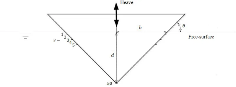
As shown in Figure 4, we consider a hull section S22 with sharp keel investigated in [17], which has

mean draught

= 9.5 m

and half of mean breadth

= 4.5 m

. The hull section harmonically rolls on

the water surface with frequencies

= 0.4~2.6 rad/s

, which covers nearly all possible frequencies

encountered in real sea waves. In the linear framework, the roll amplitude is assumed to be unit. Each

side of the wetted surface is equally divided into 60 segments, and let

= 1,2, ⋯ ,60

be indices of

segments orderly from top most one to the bottom most one under water surface.

Figure 4. A hull section S22 with sharp keel [17] harmonically rolls on the water surface, with mean draught = 9.5 m, half of mean breadth = 4.5 m, roll frequencies = 0.4~2.6 rad/s. Each side of the wetted surface is equally divided into 60 segments.

Noting that the section S22 has flare angle, we need to eliminate the numerical instability of the

TGF method. One could employ the approach proposed in the last sub-Section to do so. However,

the distribution of viscosity coefficient values in the flow field for eliminating the numerical

instability might not satisfy the requirement for capturing the viscous dissipation effects in rolls.

Therefore, in this case we adopt another approach, e.g., setting the source density on the segments

adjacent to water surface at each time step to zero [12], to eliminate the numerical instability. After

several tries, we set the source density on the first 3 segments (

= 1~3

) of each side adjacent to

water surface to zero, under the condition of which the numerical stability holds when using

TGF _V

to study rolls of the section S22.

Figure 4.A hull section S22 with sharp keel [17] harmonically rolls on the water surface, with mean draughtd=9.5 m, half of mean breadthb=4.5 m, roll frequenciesω=0.4 ∼2.6 rad/s. Each side of

the wetted surface is equally divided into 60 segments.

Noting that the section S22 has flare angle, we need to eliminate the numerical instability of the TGF method. One could employ the approach proposed in the last sub-Section to do so. However, the distribution of viscosity coefficient values in the flow field for eliminating the numerical instability might not satisfy the requirement for capturing the viscous dissipation effects in rolls. Therefore, in this case we adopt another approach, e.g., setting the source density on the segments adjacent to water surface at each time step to zero [12], to eliminate the numerical instability. After several tries, we set the source density on the first 3 segments (s=1 ∼3) of each side adjacent to water surface to zero, under the condition of which the numerical stability holds when using TGF1_V∞to study rolls of the section S22.

Here we take the roll frequency as the reference frequency in the viscosity coefficient, and set the non-dimensional viscosity coefficient ase=0.15 for the whole flow field, which can lead to pretty good results. The viscous dissipation effects generated by this viscosity coefficient are supposed to capture the pressure loss in the vicinity of sharp keel.

Figure 5a,b depicts the roll-into-roll added mass and damping coefficients, respectively. Figure5c,d depicts the roll-into-sway added mass and damping coefficients, respectively. The CFD results were obtained in [17] using solver OpenFOAM, in which the roll amplitude is fixed at 3.21◦ and significant vortex shedding phenomenon was observed. As suggested by Lavrov et al. [17], the hydrodynamic coefficients from TGF, TGF1_V1and TGF1_V∞are calculated using cosine and sine Fourier transforms of the force or moment at a steady phase.

In Figure5, one can observe that there exists significant discrepancy between inviscid TGF and CFD results, while the TGF1_V∞results agree well with the CFD ones. In fact, TGF1_V∞not only accurately predicts the roll damping by taking viscous damping that is ignored by TGF into account, but also significantly improves the added mass of the roll section S22. This result suggests that the viscous dissipation effects have an impact not only on the roll damping, but also on the added mass, though the viscous damping might dominate the influence of viscosity.

On the other hand, it is obvious that the agreement between TGF1_V1and CFD results is not as well as that between TGF1_V∞and CFD results, especially the added mass in Figure5a,c. This suggests that the spatial viscous dissipation effects (higher order viscosity coefficient) also play an important role in the whole viscous dissipation effects, which should not be ignored when the viscosity coefficient is sufficient large in the vortex shedding cases.

Water2018,10, 72 13 of 17 Here we take the roll frequency as the reference frequency in the viscosity coefficient, and set

the non-dimensional viscosity coefficient as = 0.15 for the whole flow field, which can lead to

pretty good results. The viscous dissipation effects generated by this viscosity coefficient are supposed to capture the pressure loss in the vicinity of sharp keel.

Figure 5a,b depicts the roll-into-roll added mass and damping coefficients, respectively. Figure 5c,d depicts the roll-into-sway added mass and damping coefficients, respectively. The CFD results were obtained in [17] using solver OpenFOAM, in which the roll amplitude is fixed at 3.21° and significant vortex shedding phenomenon was observed. As suggested by Lavrov et al. [17], the

hydrodynamic coefficients from TGF, TGF _V and TGF _V are calculated using cosine and sine

Fourier transforms of the force or moment at a steady phase.

(a) (b)

(c) (d)

Figure 5. Hydrodynamic coefficients of section S22 using TGF, TGF _V and TGF _V are compared with CFD results [17]. The non-dimensional viscosity coefficient in TGF _V and TGF _V is set as

= 0.15 on all segments and the roll of frequency is set as the reference frequency in viscosity

coefficient: (a) roll-into-roll added mass coefficients; (b) roll-into-roll damping coefficients; (c) roll-into-sway added mass coefficients; and (d) roll-into-sway damping coefficients.

In Figure 5, one can observe that there exists significant discrepancy between inviscid TGF and

CFD results, while the TGF _V results agree well with the CFD ones. In fact, TGF _V not only

accurately predicts the roll damping by taking viscous damping that is ignored by TGF into account, but also significantly improves the added mass of the roll section S22. This result suggests that the viscous dissipation effects have an impact not only on the roll damping, but also on the added mass, though the viscous damping might dominate the influence of viscosity.

On the other hand, it is obvious that the agreement between TGF _V and CFD results is not as

well as that between TGF _V and CFD results, especially the added mass in Figure 5a,c. This

suggests that the spatial viscous dissipation effects (higher order viscosity coefficient) also play an Figure 5.Hydrodynamic coefficients of section S22 using TGF, TGF1_V1and TGF1_V∞are compared

with CFD results [17]. The non-dimensional viscosity coefficient in TGF1_V1 and TGF1_V∞ is

set as e=0.15 on all segments and the roll of frequency ω is set as the reference frequency in

viscosity coefficient: (a) roll-into-roll added mass coefficients; (b) roll-into-roll damping coefficients; (c) roll-into-sway added mass coefficients; and (d) roll-into-sway damping coefficients.

The numerical results in this case suggest that the TGF1_V∞ can be directly employed for capturing the pressure loss of a floating body rolling on the water surface with vortex shedding in the vicinity of the sharp edge. In contrast, in works of Chen et al. [7] or Cummins and Dias [8], the GF1_V1 mainly relies on an additional pressure discharge model to capture the pressure loss. The TGF1_V1 results in this case also points out the importance of spatial viscous dissipation effects (second order viscosity coefficient), which can significantly improve the hydrodynamic coefficients with viscous dissipation effects. Moreover, as compared to those viscous damping correction methods [13,15] that only make corrections on the damping coefficient, the TGF1_V∞can consider the viscous dissipation effects not only on damping coefficient, but also on added mass coefficient.

4. Conclusions

viscous dissipation effects, while, in the existing TGF_V1, only the free-surface memory term has viscous dissipation effects.

The advantages of TGF1_V∞are demonstrated through two typical cases. One is a wedge with flare angle heaving on the water surface. The numerical results suggest that the method based on TGF1_V∞gives stable numerical results while these from the method based on the existing Green’s function (TGF1_V1) lead to divergent and/or unstable results. The results indicate that the spatial viscous dissipation effects play an important role in eliminating the numerical instability associated with the existing methods. The other case is a hull section of a ship with a sharp keel rolling on the water surface, in which vortex shedding phenomenon appears. The comparison of the results from the methods based on TGF1_V∞and the existing Green’s function with these results from CFD simulations suggests that the viscous dissipation effects have impact not only on the roll damping, but also on the roll added mass, and that the method based on the new TGF1_V∞can give much closer results to the CFD simulations.

Moreover, the newly developed instantaneous term in the TGF1_V∞has an advantage of faster decay rate than that of the existing Green’s function when the distance between the field and source points increases, which can significantly reduce the computational costs when employing it as the Green’s function of Rankine panel methods.

In the future, the time-domain Green’s functions (TGF1_V∞) for the 3D interaction between water waves and floating bodies with viscous dissipation effects will be developed to be able to solve more practical problems.

Acknowledgments: This project is supported by the National Natural Science Foundation of China (Grant No. 51509053, No. 51579056 and No. 51579051). Q. W. Ma wishes to thank the Chang Jiang Visiting Chair professorship of Chinese Ministry of Education, supported and hosted by the HEU.

Author Contributions:Zhiqun Guo and Q. W. Ma developed the time-domain Green’s function; Hongde Qin performed the numerical calculations; and Zhiqun Guo wrote the paper.

Conflicts of Interest:The authors declare no conflict of interest. The founding sponsors had no role in the design of the study; in the collection, analyses, or interpretation of data; in the writing of the manuscript, and in the decision to publish the results.

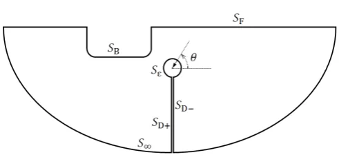
Appendix A

LetSF, SB, S∞be the water surface, wetted surface of floating body, and surrounding surface at infinity, respectively. The velocity potential at pointqat timeτis denoted byψ(τ,q). Applying Green’s theorem toψ(τ,q)andG1_n(p,t;q,τ;e), one obtains

Z t

0 dτ Z

SF+SB+S∞

ψ(τ,q)∂G1_n ∂nq

−G1_n

∂ψ(τ,q) ∂nq

dsq=2πβψ(t,q) (A1) whereβis an unknown constant decided by the instantaneous term inG1_n.

The free-surface term Ge_{1_n} is harmonic in the fluid domain, so applying Green’s theorem to ψ(τ,q)andGe_{1_n}, we have

Z t

0 dτ Z

SF+SB+S∞

ψ(τ,q)∂Ge1_n ∂nq

−Ge_{1_n}

∂ψ(τ,q) ∂nq

!

dsq=0 (A2)

Using the boundary conditions for Ge_{1_n} on S∞, it can be deduced that the integral of Equation (A2) onS∞equals to 0. Using the initial and free-surface conditions forψ(τ,q)and first kind

e

Rt 0dτ

R SF

ψ∂G_∂e_n1_n

q −Ge1_nψnq

dsq =−1g Rt

0dτ R

SF

ψ

∂2Ge1_n

∂τ∂τ −2eω

∂Ge1_n

∂τ

−Ge_{1_}n(ψττ+2eωψτ)

dsq

=−1 g R

SF

ψ∂Ge1_n

∂τ −Ge1_nψτ−2eωψGe1_n

|t

τ=0dsq =−1_gR

SFψ

∂Ge1_n

∂τ |

t

τ=0dsq

(A3)

Substituting Equation (A3) into Equation (A2) yields

Z t

0 dτ Z

SB

ψ(τ,q)∂Ge1_n ∂nq

−Ge1_n

∂ψ(τ,q) ∂nq

!

dsq= 1 g Z

SF

ψ(τ,q)∂Ge1_n ∂τ

τ=tdsq (A4)

On the other hand, substituting Equation (A2) into Equation (A1), and taking Equation (3) into account, one obtains

Z t

0 dτ Z

SF+SB+S∞

ψ(τ,q)∂ δ

(t−τ)G1_n ∂nq

−δ(t−τ)G1_n

∂ψ(τ,q) ∂nq

!

dsq =2πβψ(t,q) i.e.,

Z

SF+SB+S∞

ψ(t,q)∂G1_n ∂nq

−G1_n

∂ψ(t,q) ∂nq

!

dsq =2πβψ(t,q) or

R

SB

ψ(t,q)∂G_∂n1_n

q −G1_n

∂ψ(t,q) ∂nq

dsq−2πβψ(t,q)

= R

SF+S∞

G1_n∂ψ_∂(nt,qq)−ψ(t,q)

∂G1_n

∂nq

dsq

(A5)

Subtracting Equation (A4) from Equation (A5) yields

R

SB

ψ∂G_∂n1_n

q −G1_n

∂ψ ∂nq

dsq−R₀tdτR_S

B

ψ∂G_∂e_n1_n

q −Ge1_n

∂ψ ∂nq

dsq−2πβψ

=R

SFG1_n

∂ψ ∂ηdsq−

R

SFψ

∂G1_n

∂nq +

1 g

∂Ge_{1_n} ∂τ

τ=t

dsq −R

S∞

ψ∂G_∂n1_n

q −G1_n

∂ψ ∂nq

dsq

(A6)

If the right hand side of Equation (A6) equals to 0, i.e., G1_n= ∂G_∂n1_qn +

1 g

∂Ge_{1_n} ∂τ

τ=t

=0 on SF, and G1_n ∼O 1/rpqonS∞, the singular points can be distributed only on the wetted surfaceSB. Therefore, the definite conditions for the instantaneous termG1_n(p,q;e)can be concluded as following

           ∇2

qG1_n=βδ(p−q), p,q∈Ω

G1_n =0, η=0

G1_n ∼O

1 rpq

, rpq→∞

∂G1_n

∂η =−

1 g

∂Ge_{1_n}

∂τ , t=τ,η=0

Water2018,10, 72 16 of 17

Appendix B

̅_{_}

− ̅ _ d − d _ − _ d − 2π

= ̅ _ d −

̅ _{_} +1

g

_

= d

− ̅ _ − ̅ _ d

(A6)

If the right hand side of Equation (A6) equals to 0, i.e., ̅ _ =

̅_{_}

+ _

= = 0 on , and

̅ _{_ ~ 1⁄ on , the singular points can be distributed only on the wetted surface . Therefore,}

the definite conditions for the instantaneous term ̅_ ( , ; ) can be concluded as following

∇ ̅ _ = ( − ), , ∈

̅ _{_ = 0, = 0}

̅ _{_ ~} 1 _{, → ∞}

̅ _{_} = −1

g

_

, = , = 0

(A7)

Appendix B

Figure A1. The integral path for the instantaneous term ̅_ ( , ; ).

The harmonic characteristic of ̅ _ ( , ; ) ( ≠ ) can be easily verified. Thereby, applying

Green’s theorem to ( , ) and ̅ _ ( , ; ) yields

̅ _{_}

− ̅ _ d = 0 (A8)

Since the point locates at the upper half space, the Green’s theorem with respect to ( , )

and Re − equals to 0 and the integral of Equation (A8) on + + reduces to

̅ _{_}

− ̅ _ d

= Re −

− Re − d

(A9)

Defining = , according to Equation (15), the first term at right hand side of Equation

(A9) on can be expanded as

Figure A1.The integral path for the instantaneous termG1_∞(p,q;e).

The harmonic characteristic ofG1_∞(p,q;e)(p 6= q) can be easily verified. Thereby, applying Green’s theorem toψ(t,q)andG1_∞(p,q;e)yields

Z

SF+SB+S∞+Sε+SD++SD−

ψ∂G1_∞ ∂nq

−G1_∞ ∂ψ

∂nq !

dsq=0 (A8)

Since the pointqlocates at the upper half space, the Green’s theorem with respect toψ(t,q)and Re

E1 −e2k0Rpq equals to 0 and the integral of Equation (A8) onSε+SD++SD−reduces to

R

Sε+SD++SD−

ψ∂G_∂n1__q∞ −G1_∞∂∂ψnq

dsq

= R

Sε+SD++SD−

Re

E1 −e2k0Rpq _∂∂ψ_nq −ψ∂Re{E1(−e

2_k 0Rpq)}

∂nq

dsq

(A9)

Definingrε=

Rpq, according to Equation (15), the first term at right hand side of Equation (A9) onSεcan be expanded as

R

SεRe

E1 −e2k0Rpq _∂∂ψ_nqdsq

= R

Sε ∂ψ

∂nq −γ−ln

e2k0Rpq+O(rε)dsq rε→0

= ∂ψ(t,p) ∂nq

R2π

0 −γ−ln e2k0rε

rεdθ=0

(A10)

As shown in FigureA1, the second term at right hand side of Equation (A9) onSεcan be calculated as follows

R

Sεψ

∂Re{E1(−e2k0Rpq)}

∂nq dsq

= Rπ

0 ψRe n

expe2k0rεei( 3π

2 −θ) o

dθ

+ R2π

π ψRe n

expe2k0rεei(θ−

π 2)

o

dθrε=→02πψ

(A11)

The integral at right hand side of Equation (A9) onSD++SD−equals to 0 due to the inverse gradient direction onSD−andSD+, i.e.,

Z

S_D++SD−

RenE1

−e2k0Rpq o_∂ψ

∂nq −ψ

∂ReE1 −e2k0Rpq ∂nq

!

dsq =0 (A12) Combining Equations (A8)–(A12) yields

Z

SF+SB+S∞

ψ∂G1_∞ ∂nq

−G1_∞ ∂ψ

∂nq !

Therefore, the unknown constantβin Equations (10) and (A7) equals to

β=1 (A14)

References

1. Guével, P.Le Problème de Diffraction-Radiation—Première Partie: Théorèmes Fondamentaux; ENSM, Univ. Nantes: Nantes, France, 1982. (In French)

2. Chen, X.B. Hydrodynamics in offshore and naval applications-Part. In Proceedings of the 6th International Conference on Hydrodynamics, Perth, Australia, 24–26 November 2004.

3. Dias, F.; Dyachenko, A.I.; Zakharov, V.E. Theory of weakly damped free-surface flows: A new formulation based on potential flow solutions.Phys. Lett. A2007,372, 1297–1302. [CrossRef]

4. Chen, X.B.; Dias, F. Visco-potential flow and time-harmonic ship waves. In Proceedings of the 25th International Workshop on Water Waves and Floating Bodies (IWWWFB), Harbin, China, 9–12 May 2010. 5. Yao, C.B.; Dong, W.C. Modeling of fluid resonance in-between two floating structures in close proximity.

J. Zhejiang Univ. Sci. A (Appl. Phys. Eng.)2015,16, 987–1000. [CrossRef]

6. Qin, H.D.; Shen, J.; Chen, X.B. A free surface frequency domain Green function with viscous dissipation and partial reflections from side walls.J. Mar. Sci. Appl.2011,10, 259–264. [CrossRef]

7. Chen, X.B.; Dias, F.; Duan, W.Y. Introduction of dissipation in potential flows. In Proceedings of the 7th International Workshop on Ship Hydrodynamics, Shanghai, China, 16–19 September 2011.

8. Cummins, C.P.; Dias, F. A new model of viscous dissipation for an oscillating wave surge converter. J. Eng. Math.2017,103, 195–216. [CrossRef]

9. Wu, G. The Time-Domain Green Function Method Involving Fluid Viscosity. Master’s Thesis, Harbin Engineering University, Harbin, China, 2007.

10. Dai, Y.S.; Duan, W.Y. Potential Flow Theory of Ship Motions in Waves, 1st ed.; The National Defense Industries Press: Beijing, China, 2008; pp. 253–254. ISBN 9787118053159.

11. Faltinsen, O.; Zhao, R. Numerical predictions of ship motions at high forward speed.Philos. Trans. R. Soc. B 1991,334, 241–252. [CrossRef]

12. Duan, W.Y. Nonlinear Hydrodynamic Forces Acting on a Ship Undergoing Large Amplitude Motions. Ph.D. Thesis, Harbin Engineering University, Harbin, China, 1995.

13. Katayama, T.; Yoshioka, Y.; Kakinoki, T.; Ikeda, Y. Some topics for estimation of bilge-keel component of roll damping. In Proceedings of the 11th International Ship Stability Workshop, Wageningen, The Netherlands, 21–23 June 2010; pp. 225–230.

14. Zhang, H.; Li, J.D. Improving longitudinal motion prediction of hybrid monohulls with the viscous effect. J. Mar. Sci. Appl.2007,6, 39–45. [CrossRef]

15. Yasukawa, H. Application of a 3-D time domain panel method to ship seakeeping problems. In Proceedings of the 24th Symposium on Naval Hydrodynamics, Fukuoka, Japan, 8–13 July 2002; pp. 376–392.

16. Downie, M.J.; Dearman, P.W.; Graham, J.M.R. Effect of vortex shedding on the coupled roll response of bodies in waves.J. Fluid Mech.1988,189, 243–261. [CrossRef]

17. Lavrov, A.; Rodrigues, J.M.; Gadelho, J.; Guedes Soares, C. Calculation of hydrodynamic coefficients of ship sections in roll motion using Navier-Stokes equations.Ocean Eng.2017,133, 36–46. [CrossRef]