1
Uncertainty and bias in electronic tide-gauge records: evidence from collocated sensors
Abbreviated title: Bias in electronic tide-gauge records
Stella Pytharoulia, Spyros Chaikalisb and Stathis C. Stirosb
aDepartment of Civil and Environmental Engineering, University of Strathclyde, G1 1XJ
Glasgow, United Kingdom, corresponding author, email: stella.pytharouli@strath.ac.uk bGeodesy and Geodetic Applications Lab., Department of Civil Engineering, University of
Patras, GR 26500 Patras, Greece, email: stathis.stiros@strath.ac.uk
Abstract
Understanding noise and possible bias in tide-gauge sensors is important for determining the mean sea level, its fluctuations and their climatic, geophysical and engineering implications, but not an easy task. In the past, this problem has been examined through comparison of different sensors in the laboratory, or through correlations of neighbouring sensors. In this study we identified and studied 10 cases of harbours with fully collocated sensors. Transient differences were found between collocated records. Pressure gauges were found significantly more sensitive to noise than radar-type sensors, and with higher chances of long-term transient bias. The amplitude of the observed bias is important, of the same order of magnitude with tsunami waves in the open sea and with seismic ground displacements. Only 9% of the sensors analysed were found to satisfy the 1 cm accuracy criterion imposed by the Permanent Service for Mean Sea Level (PSMSL).
2
1.
INTRODUCTION
Tide gauges have been established in harbours since the 18th c. to provide information on the quasi-periodic tidal fluctuations of the sea level obstructing navigation. Early gauges were simple vertical metred poles fixed in quiet places of harbours. Because of their efficiency, they were also used to define the geodetic datum (zero elevation for maps) and were evolved into mechanical, continuously recording floaters. In the last 50 years, tide gauges have also been used for the study of large-scale water dynamics, as well as of various coastal, tectonic, meteorological and climatic processes (e.g. Church and White (2006), Menéndez and Woodworth (2010), Zerbini et al. (2017), Wöppelmann and Marcos, (2016); Becker et al (2016))). Recently, the new generation of electronic high-rate recording tide-gauges (with a sampling rate of a few minutes to a few seconds) have been used to monitor transient effects such as tsunami waves (e.g. Fujii and Satake (2007), Satake et al. (2013).
Two major problems with tide-gauge data are that their number at a global scale was till recently limited (at present there are approximately 2,300 operational stations worldwide; PMSL, 2017), and that the deterministic astronomic signal is mixed with an essentially stochastic meteorological signal; for this reason, there is no easy way to control noise and bias in their records, i.e. to understand what their uncertainty limits are (Chelton and Enfield, 1986). As a consequence, the uncertainty in the recordings of tide-gauges has not been resolved even for the modern, electronic tide-gauges.
3
from measurements in laboratory conditions, usually very different from those in port or open seas environments.
In this article we examined a large number of tide-gauges at global scale, identified those which can be regarded as collocated, and analysed their differences. This approach represents the optimal way to document the uncertainties/error properties of tide-gauges from real data in different hydraulic conditions and geographic environments, and is novel. This is because so far, differences between collocated operating time gauges have clearly been noticed, but they were discarded, readily assigned to outliers, a priori assuming one sensor reliable. For this reason, the statistical information provided by differences in collocated sensors was ignored.
The output of this study is to identify and classify the differences between the different types of collocated sensors using raw, unfiltered data. We aim to provide information on how each sensor type behaves, which type is the most prone to bias, how big this bias can be and whether it can be related to other external factors which, if controlled, could reduce errors.
1.1.MAIN TYPES AND FUNCTION OF TIDE-GAUGES
The most common type of tide gauge is the traditional mechanical floater. The float remains on the sea surface and is connected to a system of pulleys and weights. As the float follows the sea level fluctuations, its movement is translated to actual water level on a recording paper (IOC, 1985). A floater with encoder (ENC) is the type of tide gauge where the mechanism that translates the float movement to water level values is an electric current. In the last 20 years, the mechanical sensors were replaced by electronic sensors mainly of three types (in addition to the ENC sensors mentioned above): pressure sensors, acoustic tide-gauges and radar sensors. Their basic characteristics and principles of operation are described in IOC (2002) and are summarized below.
4
Acoustic sensors (AS) provide sea level values that are based on the time that an acoustic pulse transmitted by a sensor located directly above the sea level, requires to reach the sea surface and return back to the transmitter (time of flight). This signal is then converted to a distance from the sea surface. Acoustic pulses are, in the vast majority of cases, restricted within a vertical tube. This way, the sensor is less affected by changes in the temperature and pressure, factors that need to be taken into account for accurate sea level determination. Radar sensors (RAD) are fixed above the maximum water level and measure the distance between the fixed radar and the water level below through a radio signal reflected on the water surface. Their advantage over an acoustic sensor is that they are not affected by temperature variations (IOC, 2002).
1.2.PREVIOUS STUDIES ON UNCERTAINTIES OF TIDE-GAUGES
All types of measurements are affected by measurement errors of different types, and tide-gauges are no exception. However, till recently, the understanding of their errors was nearly impossible, because tide-gauges are isolated instruments, there is no possibility to reproduce tidal effects, and no comparisons with other records (independent constrains) were possible. For example, it was found that in certain regions wrong type of lubricants were occasionally used for mechanical floaters, and saline water had the tendency to gradually reduce the viscosity of these lubricates with time. This led to gradually increased damping and attenuation of small-amplitude oscillations, hence biasing tide-gauge records. Some of these records have been discarded, but it is unknown how many others are affected, especially because no detailed metadata are available.
tide-5
gauges and bottom pressure sensors which resulted in a similar value for the error in observations.
However, differences in the hydraulic energy along coasts are important even in nearby areas, as can be indirectly derived from significant variations of the elevation of the coastal biological zoning (Stiros and Pirazolli, 2004), and for this reason recordings of strictly non-collocated sensors are different, because they are influenced by unknown, different processes reflected in differences of local hydraulic energy of the sea water (mostly wave action).
Exploiting the emerging availability of collocated sensors Woodworth and Smith (2003) used data collected by a radar (RAD) and a bubbler pressure gauge (BPRS) in Liverpool (UK) over a period of one year at a sampling rate of 15 minutes. Linear regression revealed a small scale error between the two sensors, while the root mean square of the differences between corresponding values was of the order of 1.4 – 1.5 cm. The radar sensor seemed to be noisier than the bubbler, but both sensors had the same accuracy of 1 cm. Although the radar sensor was deemed to be biased up to 5 cm during a storm, the authors suggest that it should be considered for future projects/applications due to ease of installation and maintenance. The authors also suggest that a value of the root mean square (RMS) of the differences below 1.4 cm would ensure that the accuracy of the sensors is better than 1 cm. The latter is the accuracy requirement for all Global Sea Level Observing System (GLOSS) sensors, the global monitoring network that provides sea level data for oceanographic and climate research. Mehra et al. (2009) were also favourable towards the installation of radar sensors. Their study, based at Verem (India), was focused on two types of sensors: a radar (RAD) and a pressure (PRS) gauge. Their work highlighted the effects of atmospheric factors (atmospheric pressure, water density and rainfall) on the pressure gauge and the advantage of radar sensors over other types of sensors.
6
The effect of atmospheric variables on pressure gauges was the focus of the study by Mehra et al. (2013) who compared the data (5-minute average values) obtained by a radar (RAD) and a pressure (PRS) sensor deployed at three different locations within an area 10 km x 20 km. Each data set had a duration between 10 and 17 months. Their results revealed that the data from both types of sensors were similar if an atmospheric pressure correction was applied to the pressure sensor time series and they recommended the collection of atmospheric pressure data along with data collected by a pressure gauge for projects related to storm surges and tsunamis.
2.
METHODOLOGY
Uncertainty in measurements is defined in terms of accuracy and precision (Mikhail and Ackermann, 1976). Precision is a measure of the consistency of measured (usually repeated) values, and also an indicator of the repeatability of the measurements. Accuracy, on the other hand, defines a quasi-random difference between recorded values and a “true” value (systematic error, bias), but it can rarely be estimated, mostly through comparison with the output of instruments of much higher quality/specifications, or using external constraints. A simple and efficient strategy to estimate both precision and accuracy is to analyse the output of several fully collocated identical sensors recording the same known reference signal (natural effect, for example an oscillation). In this case, the differences between sensors define the precision while the differences between sensors’ output and the input reference signal define accuracy of each sensor (cf. Moschas et al., 2015).
Tide gauge measurements cannot be reproduced to obtain a standard deviation, and in addition, their accuracy cannot usually be estimated for lack of independent evidence of the instantaneous sea-level. If, however, two collocated tide-gauge records A and B are available, the time series of the differences of their instantaneous recordings, corrected for their central tendency value, can identify differences which originate from uncertainties (noise, bias) in one or both instruments.
7
the same low amplitude and has a flat frequency spectrum, their difference will correspond to a nearly horizontal line with limited noise (Figure 1b). More important fluctuations (Figure 1c) are likely to indicate coloured noise, i.e. a signal that contains frequencies of different amplitudes and its frequency spectrum is not flat, but it is not possible to identify which of the two is the noisy instrument.
However, if three collocated instruments A, B and C are available, there can be formed three time series of differences between two instruments, A-B, B-C, A-C. These three time series, corrected for their central tendency value, can be plotted as a function of time. If instrument C is characterized by high coloured noise, this noise will characterise time series B-C, A-C, but not the third one (A-B), as is schematically shown in Fig 1(d-f). Hence, it will be possible to identify an instrument with possible malfunction/high noise, and then analyse its noise from Figure 1e or 1f.
A requirement for such a study is that the instruments are fully collocated, so that they are affected by identical meteorological and the same long-period hydrodynamic effects; this means that they should be located in the same harbour. This is a main difference from most previous studies.
In our study we examined the global record of GLOSS tide-gauges from the Intergovernmental Oceanographic Commission (IOC) website in order to find two or three fully collocated tide gauges covering the same time interval. Then we examined the whole available time records to identify time intervals fully covered with data, in which there is evidence of important differences between them. The diverging parts of time series were then analysed in order to identify their statistical characteristics and significance.
8
Figure 1. Pattern of time series expressing the difference between records of collocated tide-gauges, indicated by A, B and C. Left column, plot of the time series of the difference between two tide gauge records A and B. (a): Idealized case of the differences between two records A and B without noise. (b): A nearly ideal case of the difference of two tide gauges containing only white noise; (c) A realistic case of A and B, containing both white and coloured (systematic, bias) noise. Right column, differences between recordings of three collocated tide gauges A, B and C, with C containing important coloured noise. The plot of the difference between A and B is a time series with small noise, while those between A-C, B-C with high noise. These three plots permit to identify the faulty behaviour of C.
2.1.DATA COLLECTION
For our study we focused on tide-gauges that are part of the Global Sea Level Observing System (GLOSS). The GLOSS station data used were obtained from the IOC website (http://www.ioc-sealevelmonitoring.org). Among the available 300 GLOSS stations worldwide, we identified about a dozen harbours with two or more collocated tide gauges. Ten stations were chosen for this study (Figure 2). The choice of the stations was based on the following criteria which ensure reliable results:
(1) complete high-rate records (at least 0.2 measurements per minute) for at least two collocated electronic sensors simultaneously operating and available for at least one year. (2) each sensor record should contain no more than 3.5% missing values in total.
9
From the study of the available data set, 3 sets containing 3 collocated tide-gauge sensors and 7 sets containing 2 collocated tides-gauge sensors were found to satisfy the specifications of our study and are summarised in Table 1. Sensors are mostly of pressure (PRS) and radar type (RAD), and only in one case, of floater type with encoder (ENC).
A preliminary investigation of the differences between the collocated sensors was made, and this led to search for metadata and to specific investigations (for example, inquiries to tide-gauge or data basis curators) in order to verify and understand the causes of differences between records (possibility of an atypical behaviour to reflect installation of a new instrument at a different level, etc.). No detailed response was possible, but what is clear, is that the policy of IOC is to check data in time due and automatically discard or repair sections of time series, so that final records are free of errors and of significant inconsistencies. This policy, however, reduces the possibility to study uncertainties and biases in raw data. For this reason, our study is based on raw data, i.e. absolute values as recorded at each sensor, without any smoothing or filtering applied. The only exceptions of filtering are the removal of certain high-frequency outliers, as noticed below, and downsampling of certain records so that compatible records for each station are formed (for Zanzibar station only, see Table 1 below).
10
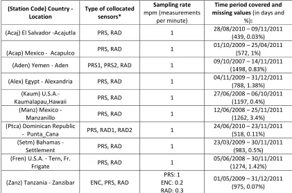
Table 1: Summary of identified and analysed stations with collocated tide gauges
(Station Code) Country -
Location Type of collocated sensors*
Sampling rate
mpm (measurements per minute)
Time period covered and missing values (in days and
%):
(Acaj) El Salvador -Acajutla PRS, RAD 1 28/08/2010 – 09/11/2011 (439, 0.03%)
(Acap) Mexico - Acapulco PRS, RAD 1 01/10/2009 – 25/04/2011 (572, 1%)
(Aden) Yemen - Aden PRS1, PRS2, RAD 1 09/10/2007 – 14/11/2011 (1498, 0.83%)
(Alex) Egypt - Alexandria PRS, RAD 1 04/11/2009 – 31/12/2011 (788, 1.38%) (Kaum) U.S.A.-
Kaumalapau,Hawaii PRS, RAD 1 27/06/2008 – 06/10/2011 (1197, 0.4%)
(Manz) Mexico -
Manzanillo PRS, RAD 1 12/06/2008 – 25/11/2011 (1262, 3.4%)
(Ptca) Dominican Republic
- Punta_Cana PRS, RAD1, RAD2 1
24/06/2010 – 23/11/2011 (518, 0.11%) (Setm) Bahamas -
Settlement PRS, RAD 1
23/03/2009 – 30/11/2011 (983, 0.5%) (Fren) U.S.A. - Tern, Fr.
Frigate PRS, RAD 1 05/06/2008 – 30/11/2011 (1274, 1.42%)
(Zanz) Tanzania - Zanzibar ENC, PRS, RAD ENC: 0.2 PRS: 1 RAD: 0.3
01/05/2009 – 31/12/2011 (975, 0.07%)
*PRS: pressure sensor, RAD: radar sensor, ENC: floater with encoder. Where more than one sensors of the same
type are found at the same location, a number is added next to the sensor type, e.g. RAD1 and RAD2.
2.2.ANALYSIS STEPS
Our methodology to provide datasets that are suitable for further evaluation can be summarised in the following steps:
2.2.1. Step 1: Homogenisation (Correction for datum differences)
11
presence of any extreme values, which may represent instrument malfunction or problems in the data logging system, and are in the focus of our analysis.
The following mathematical expression describes the homogenisation of the raw data (collocated time series for each station/harbour) into time series referring to a common datum with an acceptable precision.
X*i,j,s = Xi,j,s – mediani,j,s (eq.1)
where X* represents the homogenised values, Xi,j,s the raw data and mediani,j,s the median value in year i, from sensor s at location j, for i=1,…K year, j=1, …L location, and s=1, …S collocated sensors
2.2.2. Step 2: Calculation of the difference (bias) between collocated sensors
With the values of all collocated sensors fluctuating around zero after Step 1, the difference between two collocated sensors s1 and s2 at time t can be calculated using eq. 2:
∆𝑋 = 𝑋∗ − 𝑋∗ (eq. 2)
where 𝑋∗ and 𝑋∗ are the homogenised values at time t as calculated by eq. 1 for sensor s1 and s2, respectively. The time refers to the full duration of the data set (one year to four years). This difference represents the bias in the sea level values.
An estimate of the mean difference of the two time series is provided by the root mean square (RMS) of the differences for each pair of collocated sensors at station L
𝑅𝑀𝑆∆ =
∆
(eq. 3)
with ΔXs1s2t calculated by eq. 2 and n the total number of available pairs of observations at a specific location.
2.2.3. Step 3: Analysis of the calculated differences between collocated sensors
12
or the data logging system was investigated, using also the raw recordings for each sensor and location.
Additional analyses were made necessary at a following step in order to evaluate the results obtained.
3.
RESULTS
3.1.RANGE OF BIAS
Following the steps described in the previous section, we calculated the differences between pairs of collocated sensors for all available records and stations in Table 1 and the corresponding RMS. These results are summarized in Table 2. According to Woodworth and Smith (2003), an RMS value of 1.4 cm sets the accuracy of each sensor at 1 cm or less. The highlighted row in Table 2 corresponds to the only station and pairs of sensors among the available data which were found to satisfy this condition. The largest ranges and RMS errors correspond to station Zanzibar with the differences having a max value of 4 m and the RMS being approximately 58 cm. The smallest differences are observed at station Punta Cana with values up to 10 cm. This station exhibits the smallest RMS values (< 2 cm).
[image:12.612.94.455.475.721.2]In summary, over one billion pairs of values between collocated sensors have been used in total for our analysis. The vast majority of the differences, i.e. 80%, fall within ± 15 cm, and approximately 19.6% of the differences are extreme with an absolute value > 30 cm.
Table 2. Range of bias and corresponding root mean square (RMS) values at each station.
Station
(station code) Types of sensors Range of bias (cm) RMS of bias (cm)
Acajutla (Acaj) PRS-RAD -25 to 50 9.5
Acapulco (Acap) PRS-RAD -15 to 10 3.2
Aden (Aden) PRS1-PRS2 -30 to 90 14.7
Aden (Aden) PRS1-RAD -90 to 20 14.4
Aden (Aden) PRS2-RAD -20 to 20 5.8
Alexandria (Alex) PRS-RAD -55 to 55 28.9
Hawaii (Kaum) PRS-RAD -10 to 70 40.5
Manzanillo (Manz) PRS-RAD -100 to 100 30
Punta Cana (Ptca) PRS-RAD1 -10 to 10 1.9
Punta Cana (Ptca) PRS-RAD2 -5 to 5 1.1
Punta Cana (Ptca) RAD2-RAD1 -10 to 10 1.8
Settlement (Setm) PRS-RAD -10 to 10 2.2
Tern (Fren) PRS-RAD -50 to 70 16.4
Zanzibar (Zanz) PRS-RAD -50 to 400 58
13
Zanzibar (Zanz) RAD-ENC -50 to 300 33.8
3.2 TYPES OF BIAS
The characteristics of the differences between pairs of collocated sensors at each station, fall into one of the following categories:
3.2.1 Drift of one or more sensors (evidence of a linear trend)
Drift of one or more sensors, as evidenced by the presence of a linear trend (Míguez et al., 2012), has been observed at stations Hawaii and Tern. Both stations had the same type of collocated sensors, i.e. PRS and RAD. Figure 3 shows the differences between pairs of collocated sensors for the two stations above. The scale of the x and y axes (indicating differences between two sensors versus time) is the same for all graphs. Both stations show evidence of a linear trend in the differences for at least part of the time period examined, with the estimated slope value being statistically significant at 95% confidence level.
Table 3 presents the values of slope b of the equation
y=a+b*x (eq. 4)
where y represents the differences between sensors, x the time, a and b variables to be determined with b representing the linear trend,
14
Figure 3. Daily average values of the differences between collocated sensors PRS and RAD for Tern, U.S.A (top) and Kaumaulau, Hawaii (bottom). The highlighted areas indicate the time period and data to which a linear trend was fitted using least-squares.
Table 3. Slope of linear fit to the differences at stations Tern and Hawaii.
Station accounted for in linear Time period
regression Slope b (cm/day) ± st.error R
2
Tern June 2008 – January 2011 -0.022 ± 0.0005 0.78
Hawaii July 2008 – April 2010 -0.017 ± 0.0002 0.92
3.2.2. Sensor or data logging system malfunction
[image:14.612.94.521.360.435.2]15
16
sensor PRS1 could not record data with values below the threshold of 0.902 m (as indicated by the dashed black line).
At Aden, there was clearly a problem with the data logging system. Between February and July 2008 and March to May 2011, a series of zero values were recorded at all sensors (see Figure 4a) mostly at the same time. Where zero values were recorded at one or two sensors only, this appears as an extreme peak in the residuals (Figure 4b). In Figure 4b, positive extreme values are due to sensor PRS2 for the top plot and sensor RAD for the last two plots recording zero values. Negative extreme values are due to sensor PRS1 for the top and bottom plots and PRS2 for the plot in the middle, respectively due to zero values. It becomes evident that the two pressure gauges experience data logging problems more frequently. In addition, sensor PRS1 appears to experience a clipping effect, i.e. did not record any values smaller than 0.902 m (threshold indicated by dashed black line on PRS1 plot in Figure 4a) for the whole time period examined. This appears as an apparent periodicity in the homogenised data (Figure 4b, top and bottom plot).
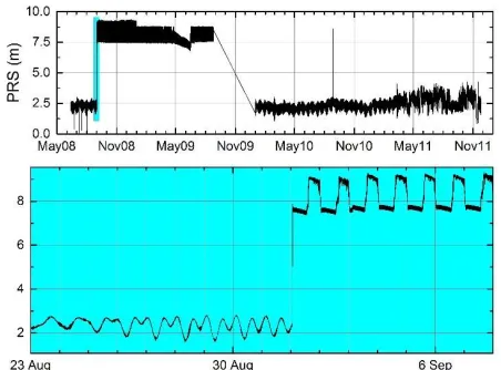
Extensive data logging problems in the form of zero values in the recordings of all sensors were also observed at Zanzibar station (Figure 5a). This can be clearly seen for RAD and ENC sensors during September - October 2010, March - May 2011 and September – December 2011. On the other hand, during those periods, sensor PRS does not appear to experience the same problem. However, a gradual increase in its sea level recordings can be observed (‘hogging’ effect). A gradual significant increase was also observed at station Tern (see Figure 3) and a gradual decrease (‘sagging’ effect) at station Acajutla.
17
Figure 5. Station Zanzibar. (a) Raw data as recorded at sensors RAD, PRS and ENC without any processing. (b) Differences between collocated sensors after removal of the median. Values fall mainly within ±10 cm up till approximately September 2011 with the exception of the differences where sensor PRS is involved.
18
In three cases, a sharp step (offset) appeared in the time series of the differences. This was the case for stations Hawaii, Manzanillo and Alexandria. The range in the amplitude of such steps was 50 cm for Hawaii (between April and May 2010, Figure 6a), 6 m for Manzanillo (September 2008 and September 2009, Figure 6b) and 40 cm for Alexandria (July 2010, Figure 6c). The lasting duration of this anomaly was 6 hours for Hawaii, 6.5 months and 1 year for Alexandria and Manzanillo, respectively.
[image:18.612.108.351.311.495.2]For Hawaii, the study of the raw sea level records (at 1 minute sampling interval) indicated that this step is due to the RAD sensor. There was a gap of 6 hours in the data for both sensors, then the datum for the RAD sensor appears to have changed by approximately 0.5 m (Figure 7). Apart from this, no other changes are observed, i.e. same range of amplitude, same waveform characteristics.
Figure 6. Sudden ‘step’ in the differences between collocated sensors PRS and RAD at stations (a) Hawaii, (b) Manzanillo and (c) Alexandria.
19
the waveform amplitudes also changed slightly. No differences in the frequency characteristics were found.
[image:19.612.111.339.221.391.2] [image:19.612.108.340.513.690.2]At station Manzanillo the jump in the differences is also due to sensor PRS. Figure 9 shows the start of the jump in the absolute sea level recordings (sampling interval = 1 minute) for PRS. It can be seen that not only there is an abrupt datum change of approximately 5 m but also the waveform is very different before and after the jump, both in the frequency and time domain.
20
Figure 8. Raw sea level data as recorded by sensor PRS at Alexandria station (top) and zoom (bottom graph) on the sharp change (highlighted area in the top graph) in the recordings. During a five-day period, three sharp changes, each occurring between consecutive samples, are visible.
Figure 9. Raw sea level data as recorded by sensor PRS at Manzanillo (top) and zoom (bottom graph) at the sharp change (highlighted area in the top graph) in the recordings. After the jump, the recorded waveform is very different compared with the time period before the jump both in amplitude and frequency.
3.2.4 Evidence of periodicity
Spectral analysis of the differences calculated at Step 2 was performed for those stations for which the residuals were visually deemed to exhibit periodic behaviour. The aim of this type of analysis was to determine whether there were any periodical effects in the residuals, and if so, what their values were. Periodical effects could represent systematic errors in the recordings of the tide-gauges.
[image:20.612.110.336.186.353.2]21
[image:21.612.109.493.316.461.2]Among the ten locations examined, stations Settlement and Zanzibar showed evidence of a periodic behaviour in the differences in the sea level between the pairs of collocated sensors. This appears as periodic fluctuations in the time series of the differences, as shown in Figure 5b RAD-ENC and PRS-ENC plots during 2009 for example. For both locations, the periodicity is observed in all pairs of collocated sensors and in their differences. A spectral analysis of the residuals at both stations revealed no statistically significant periods other to those corresponding to some of the main tidal constituents. It should be noted here that the gradient evident in both spectra of Figure 10 does not represent coloured noise, but is the result of the logarithmic scale used for both x and y axes for illustration purposes only. A linear scale in the x axis would have resulted in a nearly horizontal spectrum but for the dominant peaks.
Figure 10. Lomb normalised spectra for (a) Zanzibar and (b) Settlement stations. The period resolution of the two spectra is different due to the different length of the data sets used and their sampling rates. Some of the main tidal constituents are visible in both spectra. The scale in both x and y axes is logarithmic. The dashed line indicates the threshold above which any peaks are statistically significant at 99.9% confidence level.
4.
DISCUSSION
22
whether specific types of sensors are more prone to bias. To our knowledge, this is the first time that a systematic comparison between different types of tide gauges was made at global scale. This was made possible by comparing the data from sensors that are fully collocated, usually within a few metres from each other, and hence they record the same process without local perturbation. This section discusses our results, their significance and the implications for coastal engineering projects and earth processes studies.
4.1 AMPLITUDE OF BIAS
The differences between collocated sensors were found as high as 4 m, with the majority of the differences found to be within 15 cm, while only one pair of sensors had an RMS below 1.4 cm. This last value is suggested as the threshold below which it is ensured that each of the sensors has an accuracy better than 1 cm (Woodworth and Smith, 2003). Amongst the ten stations examined, this value was only reached at one station: Punta Cana and only two of the three sensors at this station satisfied this criterion (see Table 2).
4.2 VAN DE CASTEELE TEST (OR TEST FOR THE PRESENCE OF SYSTEMATIC ERRORS)
23
indicates white noise (compare with Figure 1a), time shift errors, instrument/system malfunction.
This test was applied to the pairs of collocated sensors at Hawaii, Manzanillo and Zanzibar, as well as Settlement station. The latter was used as a station with just white noise. Representative results from Zanzibar and Settlement stations are summarized in Figure 11. The test revealed that the differences of all examined locations are not due to time shift errors. This was the case at all but one locations (Zanzibar). Figure 11 shows the Van de Casteele plots for the differences of three pairs of collocated sensors (Figure 11a, b and c) at Zanzibar and one pair (Figure 11d) at Settlement station. The latter was used as an example of a station free of time shift errors. The resulting shapes of the Van de Casteele plots are characteristic of specific conditions. An ellipse such as that in Figure 11a, b and c is typical of a time shift between the sensors under comparison (Miguez et al., 2008). On the other hand, a straight column centred around zero as that in Figure 11d represents only instrumental noise (Miguez et al., 2008). In Figure 11b there is evidence of one more source of errors. The ellipses are not smooth but appear to have clear periodic oscillations which are representative of malfunctioning on one or both sensors (Miguez et al., 2008). The results of the Van de Casteele test for Hawaii and Manzanilo indicated different fault mechanisms. For Hawaii, the test indicated instrument malfunction while for Manzanillo a scale error (linear slope in the diagram).
24
recorded sea levels H from the sensor under testing) for selected stations: Zanzibar (a-c) and Settlement (d) stations. (a) sensor under testing: PRS, reference station: RAD. (b) sensor under testing: ENC, reference station: PRS. (c) sensor under testing: ENC, reference station: RAD. (d) sensor under testing: PRS, reference station: RAD.
4.3 SCALE ERRORS
Scale errors can be determined by linear regression analysis between the recordings of pairs of collocated sensors. One type of sensors is used as the dependent variable and the other as the independent. In this case, the slope b of the fitted line (eq. 4) can be used for the calculation of the scale error ε, as (Pérez et al., 2014):
ε = (b-1)x100 (eq. 5)
[image:24.612.94.517.563.684.2]Because our aim was to examine which type of sensors was more prone to any type of bias, no prior filtering was applied to the data, apart from removal of certain high-frequency outliers, and downsampling of the Zanzibar station records so that compatible records were formed. As a result, some of the data sets did not allow for linear regression analysis based on least-squares. The analysis was performed for all pairs of PRS and RAD sensors at six stations out of the ten available. Four stations: Tern, Alexandria, Manzanillo, Zanzibar, had a large number of extreme values, hence, they were not included in this analysis. Table 4 shows the results.
Table 4. Slope b of linear regression between pairs of PRS and RAD sensors (based on data sets with sampling interval of 1 minute) and calculated scale error. PRS was taken as independent variable and RAD as the dependent.
Station X/Y Slope, b Scale error, ε (%)
Acajulta PRS/RAD 0.9735 ± 0.0002 -2.65
Acapulco PRS/RAD 1.0165 ± 0.0002 1.65
Aden PRS2/RAD 0.9725 ± 0.0001 -2.75
Hawaii PRS/RAD 0.9949 ± 0.0003 -0.51
Punta Cana PRS/RAD1 0.9840 ± 0.0001 -1.6
Punta Cana PRS/RAD2 0.9714 ± 0.0002 -2.86
25
Table 4 reveals systematic scale differences (errors) between the PRS and RAD sensors, with the later mostly recording lower tidal ranges In the past, scale errors of the same order of magnitude have been reported (e.g. Pérez et al., 2014), while in another study pressure gauges have been associated with lower values, probably because of bias due salinity etc effects (Miguez at al., 2005).
4.4 DRIFT OR DATUM SHIFT
For two stations, Tern and Hawaii (see Figure 3), a linear trend was observed in the differences between collocated sensors. In the international literature, such linear trends are interpreted as changes in the reference datum or a drift of one of the sensors, e.g. Míguez et al. (2012), Pérez et al. (2014). The rate of change was estimated (absolute values) between 0.017cm/day (62mm/yr) and 0.022 cm/day (80 mm/yr) as shown in Table 3. All slope values computed in the analysis were significantly different from zero. Such a rate of drift is small, but when considered over a period of a year, it becomes significant. If uncorrected, it could bias the long-term trends in climate change and geological processes studies (Pérez et al., 2014).
4.5 JUMP IN THE RECORDINGS
As can be derived from Figure 6, in three out of ten stations, a sharp change in the differences between collocated sensors was observed on both types of sensors, i.e. PRS and RAD, although the PRS sensors were those affected more (in two out of the three locations). Such sharp changes had a different effect for each sensor. For the radar sensor in this study the jump is more likely associated with a change in the datum (Figure 7), most likely a result of instrument maintenance/calibration as it appeared after a gap of 6 hours in the recordings. For the pressure gauges, the jump could also indicate instrument malfunction (Figure 8 and 9).
4.5 SAGGING OR HOGGING
26
fluctuations might indicate changes in atmospheric pressure and temperature, factors that may cause significant bias in pressure gauges, if not taken into account in the transformation of readings to sea level values (e.g. Mehra et al., 2009). This could be the case for the three stations in this study, since we examined raw, uncorrected data.
4.6 PERIODIC BEHAVIOUR
Our analysis also revealed periodic components at two stations, Zanzibar and Settlement (Figure 10). Spectral analysis of the differences between collocated sensors at each location did not reveal periodicities other than those corresponding to some main tidal constituents. The absence of additional data sets e.g. meteorological data, makes it very difficult to suggest with confidence what could be affecting the pressure gauges or if there is a correlation between the ‘biased’ values and sea surges. However, a number of studies have highlighted the fact that pressure gauges are significantly affected by weather conditions (e.g. Woodworth and Smith, 2003; IOC, 2016; Mehra et al., 2009) and this could well be the case for this study.
4.7 SUMMARY OF FINDINGS
[image:26.612.108.518.634.709.2]Table 5 summarises the findings of the present analysis. The bias does not include effects such as instrumental jolts that might appear at very short time intervals (shorter than a couple of hours). Entry ‘1 or 2’ in the column ‘Number of sensors affected’ in the line ‘Datum change’ indicates that it was not possible to identify which sensor (PRS or RAD) within each pair was drifting at the two locations involved (Tern and Hawaii). Therefore, at both stations, both sensors PRS and RAD have the same likelihood to be the sensor that is drifting relative to the other. The ENC sensor is not included in Table 5 because we only had one record available and any generalisations of the results would not be precise.
Table 5. Summary of bias characteristics from this study.
Type of bias Evidenced by Amplitude of bias
Number of sensors affected PRS (out
of 11) RAD of 11)out
27
Instrument/logging
system malfunction frequency (waveform) changes - 1 0
Datum change/drift Linear trend Up to 80 mm/yr 1 or 2 1 or 2 Response to
meteorological factors
Gradual change over a time period – ‘hogging’ or ‘sagging’
Up to 1.2 m 3 0
Other Periodicity - 2 2
4.8 OVERPASSING THE NOISE PROBLEM
In the last years the number of harbours with two or more collocated tide-gauges, especially sensors with on-line data communication system, is increasing, because of the reduction of both the sensor and the maintenance cost and because of the new data communication facilities. This trend is expected to continue, and in the near future it is expected that in most harbours/locations there will be available several collocated tidal sensors. Hence, it is expected that it will be possible to compare and identify differences in sensor recordings, or even to identify faulty sensors easily.
However, care should be taken so that all sensors are fully collocated or exposed to similar environmental conditions, especially concerning the hydraulic load. This is because in main, composite harbours confluence of waves may lead for example to amplification or attenuation of the amplitude of the oscillations of the water level and to “true” tidal local differences (semi-static tidal level) which may not be representative of the “true” characteristics of the tide.
In addition, in order to control and assess in a statistical way the sensors’ output, at least in some selected sites, there should be installed and analysed sets of identical collocated sensors with a common sampling and data logging system to avoid additional noise. This will permit to compare the output. This last task, however, is not easy, because errors usually found in raw tidal data are removed and not displayed in data bases. Such modification tends to shadow important metrological information. On the contrary, raw and corrected data sets should be fully shown, as is the case in disciplines, for example in data bases used in Climatology, both raw and transformed data are both displayed and permit to understand errors and correct errors (“homogenize” data) using different approaches; for example in Global Historical Climatology Network – Monthly Version 3 (GHCN – M), available at
28
5.
CONCLUSIONS
An overall conclusion is that errors and bias were found in a small portion of tide-gauges among those existing in a global scale. The global implications of these results are high, because noise was found in nearly all cases in which data from collocated sensors permitting a systematic and reliable analysis exist. This is likely to imply that tide-gauge errors are more frequent and important than was believed before, but they cannot be identified in isolated sensors. This result may have important implications because tide gauges are used in various studies, from climatic to geotechnical engineering.
However, the trend to increase the number of collocated sensors in the last years is expected to continue and to offer redundant data to assess data quality and significance, especially through systematic study of collocated sensors operating under similar environmental conditions in selected sites. Furthermore, data bases containing both raw and corrected tidal records (and not only corrected records), as is the case in other disciplines, are necessary.
6.
FUNDING SOURCES
This research did not receive any specific grant from funding agencies in the public, commercial, or not-for-profit sectors.
7.
ACKNOWLEDGEMENTS
This paper has benefited from the comments and suggestions of two anonymous reviewers.
8.
REFERENCES
Becker, M., Karpytchev, M., Marcos, M., Jevrejeva, S. and Lennartz-Sassinek, S. (2016), Do climate models reproduce complexity of observed sea level changes? Geophysical Research Letters, 43 (10), pp. 5176-5184. DOI: 10.1002/2016GL068971.
Chelton, D. B., and D. B. Enfield (1986), Ocean signals in tide-gauge records, Journal of Geophysical Research, 91(B9), 9081–9098, doi:10.1029/JB091iB09p09081.
29
Fujii Y. and Satake K. (2007), ‘Tsunami Source of the 2004 Sumatra–Andaman Earthquake Inferred from Tide-gauge and Satellite Data’, Bulletin of the Seismological Society of America, 97(1A), S192-S207, doi: 10.1785/0120050613.
IOC (1985), ‘MANUAL ON SEA LEVEL MEASUREMENT AND INTERPRETATION, Volume I – Basic Procedures’, IOC Manuals and Guides No. 14, Volume III.
IOC (2002), ‘MANUAL ON SEA LEVEL MEASUREMENT AND INTERPRETATION, Volume III - Reappraisals and Recommendations’, IOC Manuals and Guides No. 14, Volume III.
IOC (2016), ‘MANUAL ON SEA LEVEL MEASUREMENT AND INTERPRETATION, Volume V – Radar Gauges’, IOC Manuals and Guides No. 14, Volume V.
Lentz, S. J., 1993. The accuracy of tide-gauge measurements at subtidal frequencies. Journal of Atmospheric and Oceanic Technology, 10(2), 238-245.
Mehra P., Prabhudesai R.G., Joseph A., Kumar V., Agarvadekar Y., Luis R., Damodaran S. and Viegas B. (2009), "A one year comparison of radar and pressure tide-gauge at Goa, west coast of India," International Symposium on Ocean Electronics (SYMPOL 2009), Cochin, 173-183. doi: 10.1109/SYMPOL.2009.5664190.
Mehra P., Prabhudesai R.G., Joseph A., Kumar V., Agarvadekar Y., Luis R. and Nadaf L., (2013), Comparison of sea-level measurements between microwave radar and subsurface pressure gauge deployed at select locations along the coast of India, Journal of Applied Remote Sensing, 7, 073569.
Menéndez, M., and P. L. Woodworth (2010), Changes in extreme high water levels based on a quasi-global tide-gauge data set, Journal of Geophysical Research, 115, C10011, doi:10.1029/2009JC005997.
Míguez, B.M., Gomez A.P. and Fanjul E.A. (2005), The ESEAS-RI Sea Level Test Station: Reliability and Accuracy of Different Tide-gauges, International Hydrographic Review, 6(1), 44-53.
Miguez, B.M., L. Testut, and G. Wöppelmann, (2008), The Van de Casteele Test Revisited: An Efficient Approach to Tide-gauge Error Characterization. J. Atmos. Oceanic Technol., 25, 1238–1244, https://doi.org/10.1175/2007JTECHO554.1.
30
Mikhail E.M. and Ackermann F.E. (1976), Observations and Least-squares. IEP series in Civil Engineering, New York, p. 497.
Moschas, F., Mouzoulas, D. and Stiros, S. (2015), Phase errors in accelerometer arrays: An analysis based on collocated sensors and FEM. Soil Dynamics and Earthquake Engineering, 78, pp. 32-45. DOI: 10.1016/j.soildyn.2015.07.001.
Pérez, B., Payo, A., López, D., Woodworth, P. L., and Alvarez Fanjul, E. (2014), Overlapping sea level time series measured using different technologies: an example from the REDMAR Spanish network, Nat. Hazards Earth Syst. Sci., 14, 589-610, https://doi.org/10.5194/nhess-14-589-2014.
Permanent Service for Mean Sea Level (PSMSL) (2017), "Tide-gauge Data", Retrieved 24 Aug 2017 from http://www.psmsl.org/data/obtaining/.
Press W.H., Teukolsky S.A., Vetterling W.T., Flannery B.P. (2007), Numerical Recipes: The Art of Scientific Computing, 3rd edition, Cambridge University Press, p. 1235.
Pytharouli S. and Stiros S.C. (2008), Spectral analysis of unevenly spaced or discontinuous data using the “normperiod” code. Computers and Structures, 86(1-2), 190-196.
Stiros S.C., and Pirazzoli P.A. (2004), Impact of Short-Wavelength Sea-Level Oscillations on Coastal Biological Zoning: Evidence from Nisyros Island (Aegean Sea), and Implications for the Use of the Biological Mean Sea Level as a Geodetic Datum, Journal of Coastal Research, 20(1), 244–255. JSTOR, www.jstor.org/stable/4299280.
Satake K., Fujii Y., Harada T., Namegaya Y. (2013), Time and Space Distribution of Coseismic Slip of the 2011 Tohoku Earthquake as Inferred from Tsunami Waveform Data’, Bulletin of the Seismological Society of America, 103(2B), 1473-1492, doi: 10.1785/0120120122.
Woodworth, P. L., and D. E. Smith (2003), A one year comparison of radar and bubbler tide-gauges at Liverpool. International Hydrographic Review, 4 (3), 2–9.
Zerbini S., Raicich F., Prati C.M., Bruni S., Del Conte S., Errico M., Santi E. (2017), Sea-level change in the Northern Mediterranean Sea from long-period tide-gauge time series, Earth-Science Reviews, 167, 72-87, http://dx.doi.org/10.1016/j.earscirev.2017.02.009.