1
Decentralized-Distributed Hybrid Voltage Regulation of Power Distribution Networks
Based on Power Inverters
Yu Wang
1, Yan Xu
1*, Yi Tang
1, Mazheruddin H. Syed
2, Efren Guillo-Sansano
2, and Graeme M. Burt
21 School of Electrical and Electronics Engineering, Nanyang Technological University, 50 Nanyang Ave, 639798, Singapore.
2 Department of Electronic & Electrical Engineering, University of Strathclyde, Glasgow, 16 Richmond St, Glasgow G1 1XQ, United Kingdom.
*xuyan@ntu.edu.sg
Abstract: In modern power distribution networks, voltage fluctuations and violations are becoming two major voltage quality issues due to high-level penetration of stochastic renewable energies (e.g., wind and solar power). In this paper, a hybrid control strategy based on power inverters for voltage regulation in distribution networks is proposed. Firstly, a decentralized voltage control is designed to regulate voltage ramp-rate for mitigating voltage fluctuations. As a beneficial by-product, the var capacity from the inverters become smoothed. Then, a distributed voltage control is developed to fairly utilize the var capacity of each inverter to regulate the network voltage deviations. Furthermore, once there is a shortage of var capacity from inverters, on-load tap changers control will supplement to provide additional voltage regulation support. The simulation results on IEEE 33-bus distribution network with real-world data have validated the effectiveness of the proposed voltage regulation method.
1. Introduction
In recent years, large amount of power inverter-interfaced distributed energy resources (DERs) such as solar photovoltaics (PVs) and electric vehicles (EVs) have been integrated into distributed networks [1], [2]. However, given the stochastic nature of PV generation and EV charging/discharging behavior, the distribution networks are encountering voltage limits violation and frequent voltage fluctuation [3], [4]. As pointed out in [5], the voltage fluctuations lasting ten seconds or longer at customer side should be ±3% or less, regardless of its frequency.
Conventionally, the voltage regulation is achieved by mechanical devices such as on-load tap changers (OLTCs), step voltage regulators and switched capacitors, etc. [6], [7]. However, these mechanical devices based on tap/switch actions are originally designed for distribution networks with low voltage fluctuations. For distribution networks with high DER penetration, frequent tap/switch changing of these components will reduce their lifetime dramatically [8]. As a promising alternative, the power-electronics inverters of the DERs (named power inverters hereafter) are more flexible and have much faster responding speed for generating/absorbing reactive power [9], [10]. In this regard, the IEEE 1547.8 working groups have been revising the standards to allow the inverters to contribute to voltage regulation in distribution networks [11]. Therefore, the research problem is to coordinate these power inverters for real-time voltage regulation in a high DER penetrated distribution network.
In the past, the decentralized and centralized control schemes have been widely used for voltage regulation in distribution networks [12]-[15]. The decentralized control only uses local measurement, which can be further divided into Q(V), P(V) and Q(P) strategies [12], [13]. In Q(V) or
P(V) strategy, the reactive or real power output of the inverter is dependent on the bus voltage, such as droop control [12]. While in Q(P) strategy, the reactive power output of the inverter is a function of its real power output, which is able to track the voltage fluctuation caused by PV generation intermittency [13]. The main limitation of the decentralized voltage regulation is the lack of a system-wide coordination. By contrast, the centralized control is widely proposed for voltage regulation based on optimization techniques [14], [15]. In [14], the centralized optimization of DERs and voltage regulation devices has been proposed for voltage regulation and the control signals are updated in two timescales (hourly and 15 minutes). In [15], a three-stage voltage control, which include OLTC scheduling, inverter output dispatch and real-time droop control has been proposed. However, the centralized control schemes have several limitations. First, in order to control the whole system, the parameters of distribution networks including structure, line impedance, generation and load demand is often required by the central controller. Second, the central controller suffers extensive computation and communication burdens, especially when the number of units is large. Third, the system with centralized control schemes are inherently vulnerable to communication failures, especially the single-point failure.
2 direction method of multipliers [16], [17]. An alternative
approach is the distributed coordinated control based on consensus algorithm, which can provide ‘model-free’ and ‘real-time’ solutions. In this paper, the latter approach is adopted. The intention of consensus based distributed control is to achieve fair utilization of all available devices by exchanging information via sparse communication networks. In the literature, the leader-follower algorithm has been applied to achieve distributed power dispatch for a group of wind turbines in [18] and a group of flywheel energy storage systems in [19]. The research of [18], [19] mainly focus on the power tracking control problem. In [20], a leader-follower consensus with decentralized SoC regulation is proposed for voltage rise/drop issues using distributed energy storage systems in the low-voltage distribution network. In [21], a critical bus voltage support method using electric springs based on consensus algorithm has been reported.
From the above review, most recent research only focus on the voltage limits violation problem. The voltage fluctuations problem as another important issue for network voltage regulation is not coordinately addressed in the same time. Moreover, the high fluctuations of var capacity from power inverters may distort the voltage control performance, the var capacity should also be smoothed.
This paper proposes a decentralized-distributed hybrid voltage regulation method to deal with both voltage fluctuations and limits violation issues. The technical contributions of this paper are as follows. Firstly, a decentralized voltage control is designed to regulate voltage ramp-rate for mitigating voltage fluctuations. As a beneficial by-product, the var capacity from the inverters become smoothed. Then, a distributed voltage control is developed to fairly utilize the var capacity of each inverter to regulate the network voltage deviations. Furthermore, once there is a shortage of var capacity from inverters, on-load tap changers control will supplement to provide additional voltage
regulation support. The simulation results have
demonstrated the effectiveness and advantages of the proposed method.
2. Voltage Regulation in Distribution Networks
2.1 Voltage Regulation Problem Description
In this paper, the voltage is regulated at three levels, namely, ramp-rate voltage regulation, distributed voltage regulation and OLTC voltage regulation. The ramp-rate voltage regulation aims to mitigate high-frequency voltage fluctuations. The distributed and OLTC voltage regulation aims to control the voltage deviations to eliminate voltage violation. The power inverters have fast response speed and flexible controllability, so they are used for ramp-rate and distributed voltage regulation. The mechanical devices which are not able to change frequently are used to provide additional support when there is a lack of var capacity from inverters. For a distribution network with n+1 buses denoted by i=0, 1, ..., n, bus i=0 is defined as the slack bus whose voltage can be adjusted by the OLTC. The remaining n
buses are considered as PQ buses which inject or absorb real
and reactive power. In vector form, the bus voltage magnitude deviation (ΔV=[ΔV1,…, ΔVn]T) with respect to
real power deviation (ΔP=[ΔP1, …, ΔPn]T) and reactive
power deviation (ΔQ=[ΔQ1, …, ΔQn]T) can be represented
as
VP VQ
V S P S Q (1) where SVP and SVQ are sensitivities of bus voltage
magnitudes with respect to real and reactive power injection, obtained from the inverse of Jacobian matrix [22]. An alternative approach of voltage sensitivity analysis can be found in [23]. For low-voltage distribution networks, the resistance to reactance ratio (R/X) is relatively high compared with high-voltage transmission networks, therefore, according to (1), the bus voltages are affected by both real ∆P and reactive power ∆Q changes. Especially when PV units experience shading effects, due to cloud movements, PV power output fluctuation may become severe and create significant voltage fluctuations in weak networks [24]. The power inverters can achieve fast voltage regulation through flexibly changing the ∆P and ∆Q at each bus.
The OLTC transformer at distribution substation can provide additional voltage regulation. The function of substation OLTC is to keep the voltages along the distribution networks fed by the substation within the acceptable range. Most of the OLTCs consist of an auto-transformer equipped with an on-load tap changing mechanism. The network voltages are regulated by changing taps on the series winding of the autotransformer. Conventionally, the control signals of these devices can be obtained by remote voltage measurements at voltage critical buses. The voltage deviation with OLTC in vector form is described by
VP VQ T tap
V S P S Q V (2)
where T is the tap position of the OLTC, ∆Vtap= 1
[ ,..., ]T
tap tapN
V V
is a vector representing the voltage
variation caused by each tap change to the downstream network, for the bus at the upstream network of the OLTC,
∆Vtap,i =0.
2.2 Var Capacity of Power inverters
A distribution network with N power inverters denoted by i=0, 1, ..., N is considered. The time-varying var capacity of ith power inverter can be represented as follows:
2 2
, ,
,( ) DI i DI i ( )
DI i
Q k S P k (3)
where QDI i,is the var capacity of ithpower inverter when real power output is PDI,i at interval k. SDI,i is the rated capacity of ith power inverter, which usually equals the maximum real power output of dc source.
3 var support. The oversized capacity of ith inverter S’DI,i can
be represented as follow: '
, (1 ) ,
DI i i DI i
S
S (4) where αi is the percentage of the inverter oversizing. According to (3) and (4), the variation range of var capacity, DI i
Q after oversize is:
2
, ,
, [ i 2 i DI i,(1 i) DI i] DI i
Q S S (5)
OP 1
OP 2
OP 1
OP 2
OP 3
Oversize
Oversize (a)
(c)
(b)
(d) PV type power inverter
[image:3.595.317.553.107.379.2]EV type power inverter
Fig. 1. Illustration of real power output and var capacity of PV and EV power inverter.
In this paper, the power inverters are divided into two types according to different DC sources: PV type which has unidirectional real power output, and EV type which has bidirectional real power output. The relationship of var capacity and real power output of PV and EV power inverters, as well as their operating points (OP) are illustrated in Fig. 1. For PV type power inverter, the var capacity is minimum when the real power output reaches the peak point, as shown of OP 1, and the var capacity is maximum when the real power reaches the bottom point, as shown of OP 2 in Fig.1 (a)&(b). Similarly, for EV type power inverter, the var capacity is minimum when the real power output reaches the peak point, as shown of OP 1, and the var capacity is maximum when the real power become zero, as shown of OP 2 in Fig.1 (c)&(d). Besides, OP 3 is the minimal var capacity point during the negative real power output (EV charging) period, as shown in Fig.1 (c)&(d).
3. Proposed Hybrid Voltage Control
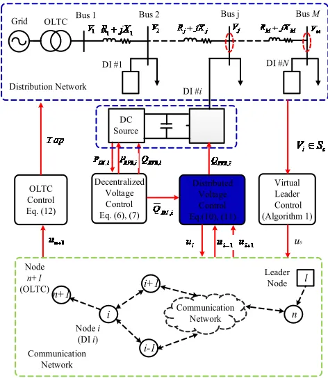
A decentralized-distributed hybrid control strategy is proposed to solve the voltage regulation problem. The control scheme diagram in Fig. 2 shows that a decentralized voltage control based on moving average filter is designed by measuring the real power output PDI,i
of inverter i. Meanwhile, the decentralized control also determines the var capacity which can be utilized by distributed voltage control. The virtual leader control collects the critical buses’ voltage information to initiate the distributed control. The leader control signal u0
spreads to all available inverters through the
communication network. In addition, OLTC control will only take effect when there is a lack of var capacity from the inverters. The details of the proposed hybrid control strategy are presented in the following subsections.
Grid
DI #1
OLTC Bus 2
DI #i Bus j
Distribution Network
l Bus M
Decentralized Voltage Control Eq. (6), (7)
Distributed Voltage Control Eq.(10), (11)
Communication Network
Leader Node
i
i-1 i+1
n DI #N Bus 1
Node i (DI i)
Virtual Leader Control (Algorithm 1)
Communication Network
n+1 Node
n+1 (OLTC)
u0 DC
Source
OLTC Control Eq. (12)
Fig. 2. The overall control architecture of proposed hybrid voltage control strategy.
3.1 Decentralized Voltage Control
The decentralized voltage control is implemented by each power inverter, which aims to locally mitigate the network voltage fluctuations and provide smooth var capacity. In this paper, a moving average filter is designed to extract high frequency components from the power variations. These variations are then compensated by both real and reactive power of the power inverter. As a result, both voltage fluctuation and remaining inverter capacity can be smoothed. At each time interval k, the moving average of the real power output of ith power inverter for window length ω is determined by
(6)
where PMA,i is the moving average value of the inverter real power output, ω is the length of the moving average window.
The moving average filter is mathematically described by the Fourier transform of the rectangular pulse as follows [26]:
A f
[ ]
| sin(
|sin(
f
f
)|
)|
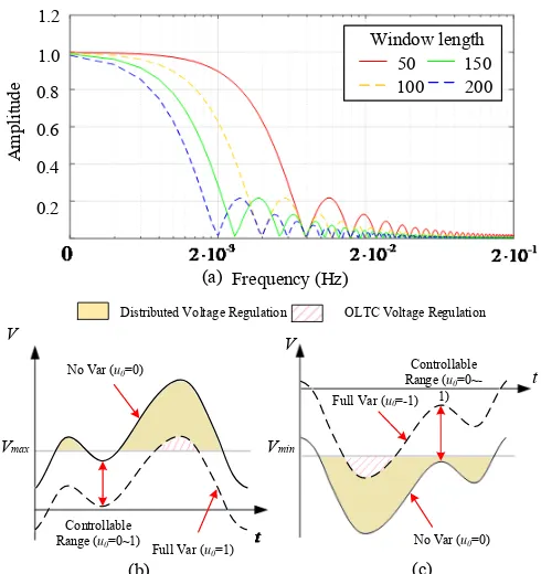
(7) where f is the signal frequency, ω is the window length, A is the amplitude of the filter frequency response. Fig. 3 (a) shows the performance of the moving average filter with different window length in frequency domain. It can be seen that the longer the moving average window length, the ,DI i Q
,
,
( ) ( )
( ) ( )
k
DI i j k MA i
P j
P k
t k t t
[image:3.595.44.291.144.354.2]4 lower the bandwidth. Therefore, less high-frequency
components will pass through the filter. In other words, the longer the window length is, the smoother the PMA,i will be
.
V
OLTC Voltage Regulation
t
No Var (u0=0)
Full Var (u0=-1)
Controllable Range (u0
=0~-1)
(b)
Full Var (u0=1)
Controllable Range (u0=0~1)
Distributed Voltage Regulation
No Var (u0=0)
V
(c)
Vmin
Vmax
Frequency (Hz)
A
m
pl
itu
de
0.6 0.8
1.0 Window length 50 150
0.4
0.2
200 100 1.2
(a)
Fig. 3. (a) Moving average filter with different window length in frequency domain. (b) Utilization state under voltage rise. (c) Utilization state under voltage drop.
The high-frequency components are extracted by subtracting the real power variations PDI,i from the moving average value PMA,i. As a result, the voltage fluctuations caused by high-frequency components of real power variations can be mitigated by the corresponding compensating real and reactive powers. To summarize, the output of the decentralized voltage control PRVR and QRVRare determined as
(8)
With (8), var capacity can be smoothed by
replacing PDI,i(k) with PMA,i(k) in (3). The smoothed var capacity from each inverter will be utilized by the distributed voltage control.
3.2 Distributed Voltage Control
In this section, a distributed voltage control based on leader-follower consensus algorithm is designed, which aims to regualte the bus voltage magnitudes within the required limits. The communication network to achieve leader-follower consensus is introduced.
Graph Theory: The communication network among the power inverters can be described by an undirected graph,
which is defined as G = (V, E) with a set of N nodes V = {v1,
v2, …,vN} and a set of edges E = V × V. Each node is assigned to a power inverter, and edges represent the communication links for data exchange. Undirected graph means communication links are bidirectional, (vi, vj) ∈ E⇒ (vj, vi) ∈E∀i, j. A matrix called adjacency matrix A = [aij] is associated with the edges. aij represents the weight for information exchanged between agents i and j, where aij=1 if agents i and j are connected through an edge (vi,vj) ∈ E, otherwise, aij = 0. For the problem of this paper, N power inverters have a virtual leader (index 0) to update their voltage regulation requirement. The interaction topology can be expressed by graph , which contains original graph G, node v0 and edges (vi, v0) from node v0 to other nodes. The
leader can send information to power inverters, but not vice versa. A pining matrix G = diag{g1, g2, …gN} is used to describe whether each inverter directly receives information from the leader, where the pinning gain gi = 1 if there is an edge (vi, v0), else gi = 0.
Consensus Condition: In this paper, the distributed voltage control is designed using the leader-follower consensus algorithm, where N power inverters will track a reference utilization state u0 provided by a virtual leader. The utilization state indicates the usage of var capacity by distributed control. The leader-follower consensus is achieved by information exchange via the communication graph defined above. The algorithm reaches consensus so that each inverter operates at an equal utilization state determined by the virtual leader. In steady-state, the utilization states between reactive power output of distributed voltage control QDVRand var capacity of all power inverters are same, i.e., the condition will be held
, ,
0 0
, ,
lim
0
DVR j DVR i
i t
DI i DI j
Q
Q
u or
u u
Q
Q
(9)Fig. 3(b) and (c) illustrates the relationship between utilization state of power inverters and network voltage profiles. As shown in Fig. 3(b), u0=0 means that there is no var support from the power inverters, while u0=1 means that there is full var support from the power inverters. In order to regulate the voltage within the allowable ranges, u0 is between 0 and 1 for over-voltage periods. Similarly, the under-voltage regulation is illustrated in Fig. 3(c), where u0
is between -1 and 0 for under-voltage periods. There are also areas where var capacity from inverters is not enough, therefore, additional voltage regualtion from OLTC is needed.
Leader Control: The reference utilization state u0 is
determined by a virtual leader measures the voltages of all critical buses in the distribution network. Firstly, the leader control will choose the maximum voltage among critical buses (denoted as Vl(k)), where the subscript
{ | max( ( ) )}
c i
i S
l i V k
, Sc is the set of the critical buses. In
this paper, the voltage critical bus refers to the bus which may have the highest/lowest voltage in the distribution network. The selection of critical buses can be based on the average highest/lowest voltage magnitudes over a certain
, , ,
, ,
,
,
, ,
, , ,
( ) ( ) ( )
if ( ) ( ) 0; ( ) 0
( ) 0
if ( ) ( ) 0. ( ) ( ) ( )
RVR i MA i DI i
MA i DI i
RVR i
RVR i
MA i DI i
RVR i MA i DI i
P k P k P k
P k P k
Q k
P k
P k P k
Q k P k P k
,
,
,( )
DI i Q k
G
[image:4.595.45.290.101.361.2]5 period of time (e.g., one month or one season). When the
information of critical buses is updated, the measurement set and communication links should also be changed correspondingly. This design ensures the voltages of critical buses are measured and controlled for network voltage regulation.
Then, based on the Vl(k) defined above, the reference
utilization state u0 is updated as follows:
0 0
0 0 0
( ) ( ( ) ), ( ) ( ) 0 ( 1) ( ) ( ( ) ), ( ) ( ) 0
0, .
s l up l up
s l low l low
u k T V k V if V k V or u k
u k u k T V k V if V k V or u k
otherwise
(10) where Vl is the maximum voltage of critical buses. Vup and Vlow are voltage upper and lower references, respectively. Ts
is the updating time interval.
In equation (10), u0 will become nonzero value once the
maximum voltage of critical buses is out of the safety operation range [Vlow, Vup] (i.e. [0.95, 1.05]).In voltage rise
period, u0 will continue updating when the condition Vl(k)>Vup or u0(k)>0 satisfied. On the contrary, u0 will
become zero again if Vl(k)≤Vup and u0(k)≤0, which means
the voltage is back to safety range and no var support from inverters is needed. Similar process is hold for voltage drop period, u0 will be updated when the condition Vl(k)<Vlow or u0(k)<0 is satisfied, and u0 will become zero again if Vl(k)≥Vup and u0(k)≥0.
Consensus Control: After u0 is calculated from (10), the utilization state of each inverter ui will be updated according to the leader-follower consensus protocol in discrete time as:
(11)
where i, j∈G. ui and uj are the utilization states of inverter i
and its neighboring inverter j, ε is a constant weight. aij is the communication coefficient between inverters i and j, and
gi is the pinning gain of the inverter i. The stability proof of the consensus control is given in [27].
Finally, the distributed voltage control output of inverter i QDVR,i is the product of its utilization state and time-vary var capacity at time interval k:
Q
DVR i,( )
k
u k Q
i( )
DI i,( )
k
(12) Noted that the smoothed var capacity obtained from the decentralized control stage will benefit the performance of distributed control since it will reduce the overshoot of reactive power output in (12).3.3 OLTC Control
The substation OLTC can change the voltage profiles of the entire downstream network in a discrete manner. If var capacity from power inverters is to be exhausted, the OLTC control will be enabled. It is assumed that there is a directed communication link between OLTC and adjacent inverter, which means that OLTC can receive the utilization state from adjacent inverter. The operation of the OLTC is defined using the following equation:
(13)
where un+1 is the utilization state received by the OLTC, a and b are parameters in the tap changing thresholds of the OLTC.
According to (13), the tap of OLTC will increase when
un+1 is larger than the upper threshold a+bTap(k), which indicates the remaining var capacity of power inverters is low and OLTC control will take effect. Similarly, the tap of OLTC will decease when un+1 is smaller than the lower threshold -a+bTap(k). In between the thresholds, the reactive power provided by power inverters is adequate for voltage regulation and therefore no tap change is required.
4. Simulation Studies
4.1 Test System
In this section, the proposed method is tested on the IEEE 33-bus distribution network [28]. The test system is implemented in Matlab/Simulink, and power flow is solved by Load Flow Tool using Newton-Raphson method. The distribution network is modified with high PV and EV penetration at selected buses as shown in Fig. 4(a). Besides, it is assumed that each power inverter only shares information with its adjacent inverters which forms a sparse communication network. The additional communication links for voltage measurement of critical buses and OLTC control are also shown in Fig. 4(a). The communication network is deployed considering the physical structure of the distribution network.
The one-hour PV generation and EV/load demand profiles used in the Scenarios 1-3 are shown in Fig. 4 (b). The PV data of 1-second resolution was measured by EPRI on June 2012 [29]. As shown in Fig. 4 (b), the PV profile ramps up and down from approximately 20% to 95% of the total PV system power rating several times within the span of an hour. The EV charging demand is assumed to be a typical residential load demand profile with smaller variation. The rated power capacity of each PV and EV system are listed in Table 2. The real power output of each power inverter can be calculated by the PV/EV profile in percentage times its power rating in MVA.
Initially, it is assumed that there is no tap change of the OLTC and the voltage at bus 1 is set to 1.0 p.u.. In this paper, the voltage limit range [Vlow, Vup] is set to [0.95, 1.05] p.u.. The initial voltage profiles of the 33-bus distribution network without any form of voltage control are shown in Fig. 4 (c) and (d). As shown in Fig. 4 (c) and (d), there are both voltage limit violations as well as severe voltage fluctuations in the distribution network. The maximum voltage deviation of bus 18 can reach 1.1 p.u. during the operation period, and the largest voltage fluctuation of bus 18 is as high as 1.1 p.u. for every ten seconds. Buses 15-18 are selected as the critical buses to initiate the distributed control once there is voltage limits violation. The performance of proposed control method is demonstrated and discussed below.
0
( 1) ( ) ( ( ) ( )) ( ( ) ( ))
i
i i ij j i i i
j N
u k u k a u k u k g u k u k
1
1
( ) 1, if ( ) ( )
( 1) ( ) 1, if ( ) ( )
( ), otherwise
n
n
Tap k u k a bTap k
Tap k Tap k u k a bTap k
Tap k
6
Table 2 Capacity of Inverters in the Test System
Power inverters Location Power rating (kVA)
PV #1 Bus 5 480
PV #2 Bus 12 840
PV #3 Bus 15 720
PV #4 Bus 18 900
PV #5 Bus 21 600
PV #6 Bus 25 360
PV #7 Bus 30 540
PV #8 Bus 32 800
EV #1 Bus 9 500
EV #2 Bus 19 300
Time (s)
0
V
ol
ta
ge
(
p.
u.)
1200 1.05
1.1
1 0.95
2400 3600
0
20 30
Bus number 33
10
Time (s)1200 0 2400
3600 0
20 30 33
10
Bus
N
um
be
r
1.1 1.08 1.06 1.04 1.02 1 0.98
(c) (d)
Time (s)
0 600 1200 1800 3600
P
er
ce
nta
ge
of
c
apa
cit
y
(%
)
0 20 40 60 80 100
EV/Load demand PV generation
2400 3000
(b)
2 1
26 27
19 33-Bus Distribution Network
20 21
28
PV #1
3 4 5 6 7 8 9 10 11 12 13 14
17 15
23 24 25
16 18 22
29 30 31 32 33
EV #1 PV #2
PV #3 PV #4
EV #2 PV #5
PV #6
PV #7 PV #8
Communication Links
(a)
Fig. 4. Basics of test system. (a) The configuration of the 33-bus distribution networks. (b) PV and EV/load profiles,
(c) Voltage profiles of the distribution network without voltage regulation, (d) The corresponding contour line.
4.2 Scenario 1
In Scenario 1, the performance of the decentralized voltage control is investigated. The simulation results of Scenario 1 are shown in Fig. 5.
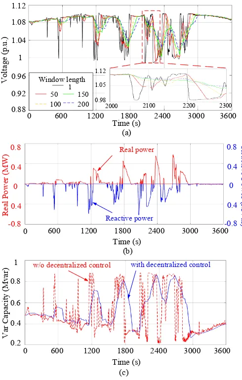
As a typical example, the voltages of bus 18 under different window length are shown in Fig. 5 (a). In Fig. 5 (a), the longer the ω is, the smoother the voltage profiles are.
The profile from 2000s to 2300s is zoomed-in in Fig. 5(a), where the largest voltage fluctuation is reduced from 10% to 3% for every ten seconds with ω>100. A conservative value of ω=150 is selected in the following part such that the voltage fluctuations are significantly smoothed.
Fig. 5 (b) and (c) show the power output of decentralized voltage control and var capacity for distributed voltage control of PV #4 (bus 18) with ω=150, respectively. According to the power output calculated by (6) and (8), real power will be curtailed and reactive power will be injected by PV #4, as shown in Fig. 5 (b). Finally, the smoothed var capacity can be obtained from (3) by replacing PDI,i(k) with moving average value in (6), as shown in Fig. 5(c). The voltage profile becomes much smoother as compared to no decentralized control (i.e. ω=1) in Fig. 5(c). This will reduce the reactive power overshoot from the distributed control and benefits the network voltage regulation.
R
ea
cti
ve
P
owe
r (
M
V
ar
)
Real power
Time (s)
R
ea
l P
ow
er
(
MW
)
-0.8 0.4 0 0.8
0 600 1200 1800 2400 3000 3600
Va
r C
apa
cit
y
(M
va
r)
0.2 0.6 0.8 1
0 600 1200 1800 2400 3000 3600
(a)
(b)
0.4
0.4
-0.8 0.4 0 0.8
0.4
Time (s)
Reactive power
w/o decentralized control with decentralized control
Time (s)
0 600 1200 2400 3600
V
olt
age
(
p.
u.)
0.88 1 1.04 1.08 1.12
0.96
0.92
1800 3000
2100 2200 2300
1.12 1.05
0.98 2000
50 150
Window length
200 100
1
(c)
Fig. 5.Results of Scenario 1. (a) Voltage profile of bus 18 with different window length, (b) Real and reactive power output of decentralized control, (c) Var capacity for distributed control.
4.3 Scenario 2
[image:6.595.310.555.267.652.2]7 is also studied where Tca changes from 0.05s to 0.1s at 1200s
and from 0.1s to 0.2s at 2400s. The simulation results of Scenario 2 are shown in Fig. 6.
The network voltage profiles with the hybrid control strategy are shown in Fig. 6 (a) and (b). Compared with Fig. 4 (c) and (d), the voltage profiles of the distribution network have significantly flattened and the voltage of buses 10-18 has been regulated within the upper voltage bound (1.05 p.u.). Besides, the voltage fluctuations have also been mitigated significantly. The total reactive power absorbed by power inverters are shown in Fig. 6 (c), where the waveform is comprised with the output of both decentralized control and distributed control. The corresponding utilization state profiles of power inverters are shown in Fig. 6 (d). The utilization states of all inverters track the utilization state determined by the leader. Besides, the utilization state of each inverter can track the leader well even when there is communication rate change at 1200s and 2400s, as shown in the enlarged view in Fig. 6 (d).
Time (s) 0
V
ol
ta
ge
(
p.
u.)
1200 1.05
1.1
1 0.95
2400 3600
0
20 30
Bus number 33
10
Time (s)1200 0 2400
3600 0
20 30 33
10
Bus
N
um
be
r
(a) (b)
Time (s)
0 600 1200 2400 3600
R
ea
cti
ve
P
ow
er
(
M
va
r)
-0.1 0.3
0.6 1 4
1 EV PV
0
1800 3000
3 2
5 8
2 7 6
0.1 0.2 0.4 0.5
Time (s)
0 600 1200 2400 3600
U
ti
li
za
ti
on S
ta
te
s
0.1 0.6 0.5
0.3
1800 3000
-0.1
(c)
(d)
1.1 1.05
1 0.95
Fig. 6. Results of Scenario 2. (a) Voltage profiles of the distribution network with the proposed hybrid control strategy, (b) The corresponding contour line, (c) Utilization states of power inverters, (d) The total reactive power output of power inverters.
4.4 Scenario 3
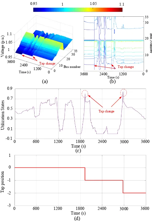
In Scenario 3, the supplementary performance of OLTC voltage regulation is tested. The parameters of (13) are set as
a=0.8, b=0.05, and Tap(k)∈[-3, 3] in this scenario. It is assumed that inverters are not oversized and hence the var capacity of the inverters is not sufficient to regulate the network voltages within the limits. Therefore, when the utilization state un+1received by OLTC reaches the upper threshold defined by (13), the tap of OLTC will be increased to provide additional voltage support. The simulation results of Scenario 3 are shown in Fig. 7 (a)-(d), where the bus voltages are regulated within the limits [0.95, 1.05]. As shown in Fig. 7 (c) and (d), once the utilization states reach the threshold defined in (13), the tap of OLTC will be triggered. During 0s≤t<1960s, the var capacity of power inverters is adequate and therefore no tap change is triggered (tap position remains at 0). During 1960s≤t<3000s, the utilization state reaches 0.8 at the 1960s and therefore tap changes to -1. It can be found in Fig. 7 (a) and (b) that there is a voltage step change of 0.1 p.u. when the control of OLTC is triggered. During 3000s≤t<3600s, the utilization state once again reaches 0.85 at 3000s and therefore the tap changes to -2, and another step change of 0.1 p.u. in the voltage can be observed in Fig. 7. Note that the proposed hybrid control strategy improves the voltage profiles in the distribution networks, while unnecessary tap changes caused by voltage fluctuation and limits violation are reduced.
Time (s) 0
V
ol
ta
ge
(
p.
u.)
1200 1.05
1.1
1 0.95
2400 3600
0 20
30
Bus number 33
10
Time (s)1200 0 2400
3600 0
20 30 33
10
Bus
N
um
be
r
1.1 1.05
1 0.95
(a) (b)
Tap change
Tap change
Time (s)
0 600 1200 2400 3600
U
ti
li
zat
io
n
St
at
es
0.1 0.7 0.5 0.3
1800 3000
-0.1
(c)
0.9
Time (s)
0 600 1200 2400 3600
T
ap
p
os
it
io
n
-2 1
0
-1
1800 3000
-3
(d)
Tap change
Fig. 7. Results of Scenario 3. (a) Voltage profiles of the distribution network with the proposed hybrid control strategy in Scenario 3, (b) The corresponding contour line,
[image:7.595.45.292.284.667.2] [image:7.595.311.557.362.720.2]8
OLTC.
4.5 Scenario 4
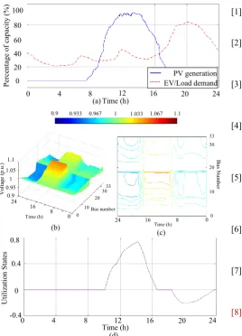
In Scenario 4, the performance of the proposed method is tested under a 24-hour operation period. It is assumed that the inverters are slightly oversized with a coefficient α=0.1. The 24-hour PV generation and EV charging/load demand profiles used in the Scenarios 4 are shown in Fig. 8 (a). There is peak PV generation in the daytime and peak load demand in the evening. The simulation results are shown in Fig. 8 (b)-(d).
[image:8.595.45.314.293.666.2]The network voltage profiles with the hybrid control strategy are shown in Fig. 8 (b) and (c). It can be observed that the network voltage can be regulated with the limits [0.95, 1.05]. The utilization state of each inverter varies for real-time voltage/var control. As the utilization states have not reach the threshold of OLTC, the tap remains unchanged. The simulation results validate the effectiveness of the proposed method for daily operation.
1.1 1.067 1.033 1 0.967 0.933 0.9
Time (h)
0 4 8 16 24
U
ti
li
za
ti
on S
ta
te
s
0 0.8
0.4
12 20
-0.4
(d) Time (h)
0 4 8 12 24
P
er
ce
nt
age
of
c
apa
ci
ty
(%
)
0 20 40 60 80 100
EV/Load demand PV generation
16 20
(a)
Time (h) 0
V
ol
ta
ge
(
p.
u.)
8 1.05
1.1
1
0.9 16 24
0 20
30
Bus number 33
10
Time (h) 8 0
16
24 0
20 30 33
10
Bus
N
um
be
r
(b)
(c)
0.95
Fig. 8. Results of Scenario 4. (a) PV and EV/load profiles,
(b) Voltage profiles of the distribution network with the proposed hybrid control strategy in Scenario 3, (c) The corresponding contour line, (d) Utilization states of power inverters.
5. Conclusion
A decentralized-distributed hybrid control strategy for voltage regulation in distribution networks has been
proposed. The decentralized voltage control utilizes the real and reactive power of power inverters to locally mitigate voltage fluctuations. The distributed voltage control coordinates all available var capacity from inverters to network voltage within limits. The OLTC control as a backup has also been incorporated into the voltage regulation architecture. The performance of the proposed control strategy has been validated in the IEEE 33-bus distribution network. The simulation results have demonstrated that the proposed method can effectively and autonomously solve voltage fluctuations and voltage rise/drop problems in distribution networks. The future work involves the validation of the proposed method experimentally. This will be done by means of a real-time controller and power hardware-in-loop setup encompassing discrete controllers, high fidelity phasor measurement unit based measurements and communication emulations.
6. References
[1] Renewables 2016 Golbal Status Report. [Online].
Available:
http://www.ren21.net/status-of-renewables/global-status-report/.
[2] W. Su, H. Eichi, W. Zeng and M. Y. Chow, “A survey
on the electrification of transportation in a smart grid environment,” IEEE Trans. Industrial Informatics, vol. 8, no. 1, pp. 1-10, Feb. 2012.
[3] J. D. Watson, et al. “Impact of solar photovoltaics on the low-voltage distribution network in New
Zealand,” IET Generation, Transmission &
Distribution, vol. 10, no .1, pp. 1-9, Jan. 2016.
[4] J. Li, C. Li, Y. Xu, Z.Y. Dong, and K.P. Wong, “Noncooperative game-based distributed charging control for plug-in electric vehicles in distribution networks,” IEEE Trans. Industrial Informatics, vol.99, no.99, 2017.
[5] “1C. 5.1, Section 4.3” in Pacific Power Engineering Handbook. [Online]. Available:
https://www.pacificpower.net/content/dam/pacific_pow er/doc/Contractors_Suppliers/Power_Quality_Standards /1C_5_1_PF.pdf
[6] M. E. Elkhatib, R. El Shatshat, and M. M. A. Salama, “Optimal control of voltage regulators for multiple feeders,” IEEE Trans. Power Delivery, vol. 25, no. 4, pp. 2670-2675, Dec. 2009.
[7] S. Hashemi and J. Østergaard, “Methods and strategies for overvoltage prevention in low voltage distribution systems with PV,” IET Renewable Power Generation, vol. 11, no .2, pp. 205-214, Nov. 2016.
[8] G. R. Mouli, P. Bauer, T. Wijekoon, A. Panosyan, and E. M Bärthlein, “Design of a power-electronic-assisted OLTC for grid voltage regulation,” IEEE Trans. Power Delivery, vol. 30, no. 3, pp.1086-1095, Jun. 2015. [9] P. M. S. Carvalho, P. F. Correia, and L. A. F. Ferreira,
“Distributed reactive power generation control for voltage rise mitigation in distribution networks,” IEEE Trans. Power Systems., vol. 23, no. 2, pp. 766–772, May 2008.
9
IEEE Trans. Power Systems, vol. 30, no. 6, pp. 3234– 3245, Jan. 2015.
[11] 1547 Series of Interconnection Standards, IEEE SCC21 Standards Coordinating Committee on Fuel Cells, Photovoltaics, Dispersed Generation, and Energy
Storage, IEEE Standards Association.
[Online].Available:
http://grouper.ieee.org/groups/scc21/dr_shared/. [12] A. O'Connel and A. Keane, “Volt–var curves for
photovoltaic inverters in distribution systems,” IET Generation, Transmission & Distribution, vol. 11, no .3, pp. 730-739, Feb. 2017.
[13] M. J. E. Alam, K. M. Muttaqi, and D. Sutanto, “A multi-mode control strategy for VAr support by solar PV inverters in distribution networks,” IEEE Trans. Power Systems, vol. 30, no. 3, pp. 1316-1326, May 2015.
[14] Y. Xu, Z. Y. Dong, R. Zhang, and D. J. Hill, “Multi-timescale coordinated voltage/var control of high renewable-penetrated distribution networks,” IEEE Trans. Power System, in press, 2017.
[15] C. Zhang, et al. “Three-Stage Robust Inverter-Based Voltage/Var Control for Distribution Networks with High-Level PV,” IEEE Trans. Smart Grid, in press, 2017.
[16] H. Almasalma, J. Engels, and G. Deconinck, “Dual-decomposition-based peer-to-peer voltage control for
distribution networks,” CIRED-Open Access
Proceedings Journal, pp. 1718-1721, Nov. 2017. [17] P. Šulc, S. Backhaus, and M. Chertkov, “Optimal
distributed control of reactive power via the alternating direction method of multipliers,” IEEE Trans. Energy Conversion, no. 29, vol. 4, pp. 968-977, Dec. 2014. [18] S. Baros and M. D. Ilic “Distributed torque control of
deloaded wind DFIGs for wind farm power output regulation,” to be published in IEEE Trans. Power Systems.
[19] Q. Cao, et al. “Coordinated control for flywheel energy storage matrix systems for wind farm based on charging/discharging ratio consensus algorithms,” IEEE Trans. Smart Grid, no. 7, vol. 3, pp. 1259-1267, May, 2016.
[20] Y. Wang, K. T. Tan, and P. L. So, “Coordinated control of distributed energy storage systems for voltage regulation in distribution networks,” IEEE Trans. Power Delivery, vol. 31, no. 3, pp. 1132-1141, Jun. 2016.
[21] Y. Zheng, et al. “Critical bus voltage support in distribution systems with electric springs and responsibility sharing,” IEEE Trans. Power Systems, no. 32, vol. 5, pp. 3584-3593, Sep. 2017.
[22] T. T. Ku, et al. “Coordination of PV inverters to mitigate voltage violation for load transfer between distribution feeders with high penetration of PV installation,” IEEE Trans. Industry Applications, vol. 52, no .2, pp. 1167-1174, Mar. 2016.
[23] B. B. Zad, J. Lobry, and F. Vallée, “A centralized approach for voltage control of MV distribution systems using DGs power control and a direct sensitivity analysis method,” Energy Conference (ENERGYCON), 2016 IEEE International, 2016.
[24] Ding, Tao, et al. “Evaluating maximum photovoltaic integration in district distribution systems considering
optimal inverter dispatch and cloud shading conditions,” IET Renewable Power Generation, vol. 11, no. 1, pp. 165-172, Aug. 2016.
[25] S. Alyami, Y. Wang, C. Wang, J. Zhao and B. Zhao, “Adaptive real power capping method for fair overvoltage regulation of distribution networks with high penetration of PV systems,” IEEE Trans. Smart Grid, vol. 5, no. 6, pp. 2729-2738, Nov. 2014.
[26] S. W. Smith, “Chapter 15 moving average filters” in
The Scientist and Engineer's Guide to Digital Signal Processing. San Diego, CA, USA: California Technical Pub., 1997.
[27] Z. Qu, “Chapter 5 Cooperative Control of Linear Systems” in Cooperative Control of Dynamic Systems: Applications to Autonomous Vehicles. New York, NY, USA: Springer-Verlag, 2009.
[28] M. E. Baran and F. F. Wu, “Network reconfigurationin distribution systems for loss reductionand load balancing,” IEEE Trans. Power Delivery, vol. 4, no. 2, pp. 1401-1407, Apr. 1989.